How accurately can a single molecule be localized in three dimensions using a fluorescence microscope?

Abstract

Single molecule fluorescence microscopy is a relatively novel technique that is used, for example, to study the behavior of individual biomolecules in cells. Since a single molecule can move in all three dimensions in a cellular environment, the three dimensional tracking of single molecules can provide valuable insights into cellular processes. It is therefore of importance to know the accuracy with which the location of a single molecule can be determined with a fluorescence microscope. We study this performance limit of a fluorescence microscope from a statistical point of view by deriving the Fisher information matrix for the estimation problem of the location of the single molecule. In this way we obtain a lower bound on the standard deviation of any reasonable (unbiased) estimation method of the location parameters. This lower bound provides a fundamental limit on the accuracy with which a single molecule can be localized using a fluorescence microscope and is given in terms of such quantities as the photon detection rate of the single molecule, the acquisition time, the numerical aperture of the objective lens etc. We also present results that show how factors such as noise sources, detector size and pixelation deteriorate the fundamental limit of the localization accuracy. The present results can be used to evaluate and optimize experimental setups in order to carry out three dimensional single molecule tracking experiments and provide guidelines for experimental design.

1. INTRODUCTION

Single molecule microscopy is a technique that can be used to study the behavior of individual biomolecules in biological specimen such as cells. This technique provides information that is seldom available through bulk studies due to averaging effects.^1,2 Hence it holds the promise to provide new insights into biological processes. One of the fundamental issues in single molecule data analysis concerns the accuracy with which the location of a single molecule can be determined. This not only gives the level of accuracy that can be obtained in an experimental setup, but it also helps in determining the nature and type of studies that can be carried out. Since the movement of a single molecule can be imaged in all three dimensions, for example, in a cellular environment,³ it is therefore important to determine the three dimensional localization accuracy of a single molecule that can be attained in a given experimental setup.

In this paper, we use the tools of statistical estimation theory^4,5 to derive an analytical expression for the fundamental limit to the three dimensional localization accuracy of a single molecule. We also derive expressions that show how experimental factors such as pixelation and noise sources affect the fundamental limit. The novel aspect of this apporach is that the limit of the localization accuracy for a given experimental condition cannot be surpassed by any unbiased estimation technique that is used to determine the single molecule location from the acquired data. In the past, there have been reports that have addressed the three dimensional localization accuracy problem of a single molecule by analyzing the performance of a specific estimation procedure.^6-8 Hence the scope of these reports is limited to the particular estimation technique used. In constrast, our approach provides a performance limit to determining the location of a single molecule. Recently, a limit to the localization accuracy of the z coordinate of a point source was reported⁹ in the context of axial tracking of a fluorescent nano-particle. This report assumed that the x and y coordinates of the point source are known. Further, the report considered a pixelated detector and evaluated the limit of the localization accuracy for different values of signal to noise ratio, which was assumed to be the same for all values of defocus distance. In the present work, we assume that all the three coordinates of the single molecule are unknown, and consider a pixelated and a non-pixelated detector. We note that the results for the non-pixelated detector provide insight into how pixelation affects the limit of the localization accuracy. Moreover, we consider a detailed noise model for the acquired data by taking into account measurement and scattering noise, which, for example, arise due to the readout process in a CCD camera¹⁰ and autofluorescence from the sample, respectively. We note that the present results are extensions of our recently published results¹¹ that address the problem of the two dimensional localization accuracy of a single molecule.

2. FUNDAMENTAL LIMIT TO THE LOCALIZATION ACCURACY

We consider a basic optical setup in which a single molecule located in the specimen space is imaged by the microscope lens system, and the image of the single molecule is captured by a detector that is located in the image space (see Fig. 1). Here, the detector collects photons from the single molecule during a fixed time interval [t₀, t]. Since the photon emission process is inherently a random phenomenon,¹² the acquired image is stochastic in nature. By using a specific estimation technique the 3D location of the single molecule can be determined from the acquired image. In an estimation problem it is important to know whether the estimation technique used to determine the unknown parameter comes close to a performance limit. This can be determined by calculating the Fisher information matrix^{4, 5} for the underlying stochastic process that describes the acquired data. The Fisher information matrix plays a crucial role in evaluating the performance of estimation algorithms. A classical result of estimation theory, namely the Cramer-Rao inequality,^{4, 5} states that the (co)variance (matrix) of any unbiased estimator θ̂ of an unknown (vector) parameter θ is bounded from below by the inverse of the Fisher information matrix I(θ), i.e.,

$$\mathrm{Cov}\left(\widehat{\theta }\right)\ge {\mathbf{I}}^{-1}\left(\theta \right).$$

Since the accuracy of an estimator is typically given in terms of the standard deviation of its estimates, the square root of the inverse Fisher information matrix provides a lower bound to the best possible accuracy. In the present context this implies that for any unbiased estimator of the single molecule location, the square root of the inverse Fisher information matrix provides a limit to the accuracy with which the location of a single molecule can be determined. We note that the Fisher information matrix is independent of estimation techniques used to determine the unknown parameter and only depends on the statistical nature of the acquired data.

Figure 1.

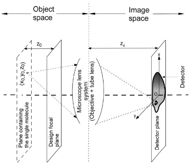
The schematic shows the main components of a fluorescence microscope imaging setup. Here, a single molecule is located at (x₀, y₀, z₀) in the object space and the image of the single molecule is captured by a detector that is located in the image space.

Due to its stochastic nature, the acquired data is modeled as a space-time random process.¹³ The temporal part describes the time points of the detected photons and is modeled as a temporal Poisson process with intensity function Λ_θ. The spatial part describes the spatial coordinates of the arrival location of the detected photons and is modeled as a family of independent and identically distributed random variables with probability density given by

$$f_{\theta }\left(r\right):=\frac{1}{M^2}{q}_{z_0}\left(\frac{x}{M}-x_0,\frac{y}{M}-y_0\right),r=\left(x,y\right)\in {ℝ}^2,\theta \in \mathrm{\Theta },$$ (1)

where Θ denotes the parameter space, M denotes the lateral magnification of the microscope lens system, (x₀, y₀, z₀) denotes the 3D location of the single molecule in the object space and q_z0 denotes the image function of a single molecule. The image function q_z0 describes the image of a single molecule on the detector plane at unit lateral magnification when the single molecule is located on the z axis in the object space (see Fig. 1). We assume that the probability density function f_θ satisfies certain regularity conditions⁴ that are necessary for the calculation of the Fisher information matrix.

According to scalar diffraction theory, the image of a single molecule that is located at (0, 0, z₀) in the object space and imaged by a fluorescence microscope can be modeled as^14-17

$$I_{z_0}\left(x,y,z_d\right)={\mid \frac{C}{z_d}{\mathit{\int }}_0^1{J}_0\left(\mathit{ka}\rho \frac{\sqrt{x^2+y^2}}{z_d}\right)\exp \left(j{W}_{z_0}\left(\rho \right)\right)\rho d\rho \mid }^2,$$ (2)

where (x, y) ∈ ℝ² denotes an arbitrary point on the detector plane, z_d denotes the axial distance of the detector from the back focal plane of the microscope lens system, C is a constant with complex amplitude, k = 2π/λ, λ denotes the wavelength of the detected photons, a denotes the radius of the limiting aperture of the microscope projected onto the back focal plane of the lens system, J₀ denotes the zeroth order Bessel function of the first kind and W_z0 (ρ) denotes the phase aberration term. We note that eq. 2 provides a general expression for several 3D point spread function models,¹⁴ which describe the image of a point-source/single-molecule and are based on scalar diffraction theory.

Rewriting eq. 2 as an image function, the image of a single molecule is given by

$$q_{z_0}\left(x,y\right)=\frac{1}{C_{z_0}}\left(U_{z_0}^2\left(x,y\right)+V_{z_0}^2\left(x,y\right)\right),\left(x,y\right)\in {ℝ}^2,z_0\in ℝ,$$ (3)

where

$$\begin{array}{c}{U}_{z_0}\left(x,y\right):={\mathit{\int }}_0^1{J}_0\left(ka\rho \sqrt{\frac{x^2+y^2}{z_d}}\right)\cos \left(W_{z_0}\left(\rho \right)\right)\rho d\rho ,\left(x,y\right)\in {ℝ}^2,z_0\in ℝ,\\ V_{z_0}\left(x,y\right):={\mathit{\int }}_0^1{J}_0\left(ka\rho \sqrt{\frac{x^2+y^2}{z_d}}\right)\sin \left(W_{z_0}\left(\rho \right)\right)\rho d\rho ,\left(x,y\right)\in {ℝ}^2,z_0\in ℝ,\\ C_{Z_0}={\mathit{\int }}_{{ℝ}^2}\left(U_{z_0}^2\left(x,y\right)+V_{z_0}^2\left(x,y\right)\right)\mathit{dxdy},z_0\in ℝ.\end{array}$$ (4)

The term C_z0 is the normalization constant, and the 1/C_z0 scaling in eq. 3 ensures that ${\mathit{\int }}_{{ℝ}^2}{f}_{\theta }\left(r\right)dr=\left(1/M^2\right){\mathit{\int }}_{{ℝ}^2}{q}_{z_0}\left(\frac{x}{M}-x_0,\frac{y}{M}-y_0\right)\mathit{dxdy}=1,\theta \in \mathrm{\Theta }$.

From eq. 3 we see that the image function q_z0 is laterally symmetric for every z₀ ∈ ℝ, i.e., q_z0 (x, y) = q_z0 (−x, y) = q_z0 (x, −y), (x, y) ∈ ℝ², z₀ ∈ ℝ. By definition ∂f_θ(r)/∂Λ₀ = 0, r ∈ ℝ², θ ∈ Θ and it can be easily shown that ∂f_θ(r)/∂x₀ = ∂f_θ(r)/∂x, ∂f_θ(r)/∂y₀ = ∂f_θ(r)/∂y for r = (x, y) ∈ ℝ², θ ∈ Θ. Here we assume that ∂Λ_θ(τ)/∂ζ₀ = 0 for τ ≥ t₀ and ζ₀ ∈ {x₀, y₀, z₀}. Further, we also assume that the partial derivative ∂q_z0/∂z₀ is laterally symmetric, i.e., ∂q_z0 (x.y)/∂z₀ = ∂q_z0 (−x, y)/∂z₀ = ∂q_z0 (x, −y)/∂z₀, (x, y) ∈ ℝ² and z₀ ∈ ℝ. This assumption is typically satisfied for most 3D point spread function models¹⁴ that are based on scalar diffraction theory. For the above conditions, the Fisher information matrix for the space-time random process that describes the acquired image captured during the time interval [t₀, t] is given by

$$\mathrm{I}\left(\theta \right)=\left[\begin{array}{cccc}{\varphi }_{\theta }\left(t\right){\mathit{\int }}_{{ℝ}^2}\frac{1}{q_{z_0}\left(x,y\right)}{\left(\frac{\partial q_{z_0}\left(x,y\right)}{\partial x}\right)}^2\mathit{dxdy}& 0& 0& 0\\ 0& {\varphi }_{\theta }\left(t\right){\mathit{\int }}_{{ℝ}^2}\frac{1}{q_{z_0}\left(x,y\right)}{\left(\frac{\partial q_{z_0}\left(x,y\right)}{\partial y}\right)}^2\mathit{dxdy}& 0& 0\\ 0& 0& {\varphi }_{\theta }\left(t\right){\mathit{\int }}_{{ℝ}^2}\frac{1}{q_{z_0}\left(x,y\right)}{\left(\frac{\partial q_{z_0}\left(x,y\right)}{{\partial }_{z_0}}\right)}^2\mathit{dxdy}\\ 0& 0& 0& {\mathit{\int }}_{t_0}^t\frac{1}{{\Lambda }_{\theta }\left(\tau \right)}{\left(\frac{\partial {\Lambda }_{\theta }\left(\tau \right)}{\partial {\Lambda }_{\theta }}\right)}^{2}d\tau \end{array}\right],$$ (5)

where

$${\varphi }_{\theta }(t):={\mathit{\int }}_{t_0}^t{\mathrm{\Lambda }}_{\theta }(\tau )d\tau ,\tau \ge t_0,\theta \in \mathrm{\Theta }.$$ (6)

The detailed derivation of the above result has been omitted due to space limitations, but can be found in a forthcoming publication.¹⁸ In deriving eq. 5, we have assumed that the unknown parameter vector is given by θ = (x₀, y₀, z₀, Λ₀). Here, Λ₀ denotes a scalar parameter that parameterizes the intensity function Λ_θ, which, for example, could be the photon detection rate of the single molecule. For the image function given in eq. 3, the partial derivatives of q_z0 (x, y) with respect to x, y and z₀ are given by

$$\begin{array}{c}\frac{\partial q_{z_0}\left(x,y\right)}{\partial \zeta }=\frac{2}{C_{z_0}}\left(U_{z_0}\left(x,y\right)\frac{\partial U_{z_0}\left(x,y\right)}{\partial \zeta }+V_{z_0}\left(x,y\right)\frac{\partial V_{z_0}\left(x,y\right)}{\partial \zeta }\right),\left(x,y\right)\in {ℝ}^2,z_0\in ℝ,\zeta \in \left\{x,y\right\},\\ \frac{\partial q_{z_0}\left(x,y\right)}{{\partial }_{z_0}}=-\frac{U_{z_0}^2\left(x,y\right)+V_{z_0}^2\left(x,y\right)}{C_{z_0}^2}\frac{\partial C_{z_0}}{{\partial }_{z_0}}+\frac{2}{C_{z_0}}\left(U_{z_0}\left(x,y\right)\frac{\partial U_{z_0}\left(x,y\right)}{{\partial }_{z_0}}+V_{z_0}\left(x,y\right)\frac{\partial V_{z_0}\left(x,y\right)}{{\partial }_{z_0}}\right),\left(x,y\right)\in {ℝ}^2,z_0\in ℝ,\end{array}$$ (7)

where

$$\begin{array}{c}\frac{\partial U_{z_0}\left(x,y\right)}{\partial \zeta }=-\frac{ka\zeta }{z_d\sqrt{x^2+y^2}}{\mathit{\int }}_0^1{J}_1\left(ka\rho \frac{\sqrt{x^2+y^2}}{z_d}\right)\cos \left(W_{z_0}\left(\rho \right)\right){\rho }^{2}d\rho ,\left(x,y\right)\in {ℝ}^2,z_0\in ℝ,\zeta \in \left\{x,y\right\},\\ \frac{\partial V_{z_0}\left(x,y\right)}{\partial \zeta }=-\frac{ka\zeta }{z_d\sqrt{x^2+y^2}}{\mathit{\int }}_0^1{J}_1\left(ka\rho \frac{\sqrt{x^2+y^2}}{z_d}\right)\sin \left(W_{z_0}\left(\rho \right)\right){\rho }^{2}d\rho ,\left(x,y\right)\in {ℝ}^2,z_0\in ℝ,\zeta \in \left\{x,y\right\},\\ \frac{\partial U_{z_0}\left(x,y\right)}{{\partial }_{z_0}}=-{\mathit{\int }}_0^1{J}_0\left(ka\rho \frac{\sqrt{x^2+y^2}}{z_d}\right)\sin \left(W_{z_0}\left(\rho \right)\right)\frac{\partial W_{z_0}\left(\rho \right)}{{\partial }_{z_0}}\rho d\rho ,\left(x,y\right)\in {ℝ}^2,z_0\in ℝ,\\ \frac{\partial V_{z_0}\left(x,y\right)}{{\partial }_{z_0}}={\mathit{\int }}_0^1{J}_0\left(ka\rho \frac{\sqrt{x^2+y^2}}{z_d}\right)\cos \left(W_{z_0}\left(\rho \right)\right)\frac{\partial W_{z_0}\left(\rho \right)}{{\partial }_{z_0}}\rho d\rho ,\left(x,y\right)\in {ℝ}^2,z_0\in ℝ,\\ \frac{\partial C_{z_0}}{{\partial }_{z_0}}=2{\mathit{\int }}_{{ℝ}^2}\left(U_{z_0}\left(x,y\right)\frac{\partial U_{z_0}\left(x,y\right)}{{\partial }_{z_0}}+V_{z_0}\left(x,y\right)\frac{\partial V_{z_0}\left(x,y\right)}{{\partial }_{z_0}}\right)\mathit{dxdy},z_0\in ℝ.\end{array}$$

Inverting the Fisher information matrix given in eq. 5 and taking the square root of the leading diagonal elements, the fundamental limit to the 3D localization accuracy of the location coordinates (x₀, y₀, z₀) of the single molecule are given by

$${\delta }_{x_0}^{3d}={\delta }_{y_0}^{3d}=\frac{1}{\sqrt{{\varphi }_{\theta }(t)}}{\left[{\mathit{\int }}_{{ℝ}^2}\frac{1}{q_{z_0}(x,y)}{\left(\frac{\partial q_{z_0}(x,y)}{\partial x}\right)}^2\mathit{dxdy}\right]}^{-\frac{1}{2}},$$ (8)

$${\delta }_{z_0}^{3d}=\frac{1}{\sqrt{{\varphi }_{\theta }(t)}}{\left[{\mathit{\int }}_{{ℝ}^2}\frac{1}{q_{z_0}(x,y)}{\left(\frac{\partial q_{z_0}(x,y)}{\partial z_0}\right)}^2\mathit{dxdy}\right]}^{-\frac{1}{2}},$$ (9)

and the fundamental limit to the accuracy of Λ₀ is given by

$${\delta }_{{\mathrm{\Lambda }}_0}^{3d}={\left[{{\mathit{\int }}_{t_0}^t\frac{1}{{\mathrm{\Lambda }}_{\theta }(\tau )}\left(\frac{\partial {\mathrm{\Lambda }}_{\theta }(\tau )}{\partial {\mathrm{\Lambda }}_0}\right)}^{2}d\tau \right]}^{-\frac{1}{2}}.$$

We refer to the above results as fundamental, since the model that is used to derive the above expressions does not take into account deteriorating factors such as pixelation and noise sources. Moreover, the model is such that all photons originating from the single molecule that reach the detector plane are detected by the detector. Note that the expressions for the fundamental limit to the 3D localization accuracy that are given in eqs. 8 and 9 depend on the z coordinate of the single molecule z₀, which we refer to as the defocus distance. As a special case, consider the in-focus scenario where z₀ is known and is equal to 0 (i.e., the plane containing the single molecule coincides with the design focal plane; see Fig. 1). For this case, the image function given in eq. 3 reduces to the classical Airy profile that is given by $q(x,y):=(J_1^2(\alpha \sqrt{x^2+y^2})/(\pi (x^2+y^2)),(x,y)\in {ℝ}^2$, where α := (2πNA/λ) and NA denotes the numerical aperture of the objective lens. Substituting this in eq. 8, we obtain the fundamental limit to the 2D localization accuracy of the single molecule that is given by

$${\delta }_{x_0}^{2d}={\delta }_{y_0}^{2d}=\frac{1}{\alpha \sqrt{{\varphi }_{\theta }(t)}}=\frac{\lambda }{2\pi \mathit{NA}\sqrt{{\varphi }_{\theta }(t)}},$$ (10)

which was reported elsewhere.¹¹

We now illustrate the results derived in this section by considering the phase aberration term W_z0 to be

$$W_{z_0}(\rho ):=\frac{\pi {(\mathit{NA})}^2{z}_0}{n_{\mathit{oil}}\lambda }{\rho }^2,\rho \in (0,1),z_0\in ℝ,$$ (11)

where NA denotes the numerical aperture of the objective lens, and n_oil denotes the refractive index of the immersion oil. The above expression for W_z0 describes the phase aberration that arises when the point source is ‘out of focus’ with respect to the detector, and corresponds to the classical ‘Born and Wolf’ 3D point spread function model.¹⁷ When analyzing data from single molecule experiments, the intensity function Λ_θ is typically assumed to be a constant. Hence in the present context, the intensity function is given by Λ_θ(τ) := Λ₀, τ ≥ t₀ where Λ₀ denotes the photon detection rate of the single molecule.

Figure 2A shows the behavior of the fundamental limit of the 3D localization accuracy ${\delta }_{x_0}^{3d}$ ( ${\delta }_{y_0}^{3d}$) of the x₀ (y₀) coordinate as a function of the defocus distance z₀. From the figure we see that at z₀ = 0, ${\delta }_{x_0}^{3d}$ coincides with the 2D fundamental limit ${\delta }_{x_0}^{2d}$ that is given by eq. 10. This is expected, since at zero defocus distance the image of the single molecule that is given by eq. 2 reduces to the Airy profile. As the value of z₀ increases (decreases), the 3D fundamental limit ${\delta }_{x_0}^{3d}$ deteriorates monotonically up to z₀ = ±1000 nm. For defocus distances greater (smaller) than 1000 nm (-1000 nm), ${\delta }_{x_0}^{3d}$ deteriorates with an oscillatory behavior. Note that the behavior of ${\delta }_{x_0}^{3d}$ is symmetric about z₀ = 0. This is expected, since the image function q_z0 corresponding to the phase aberration term W_z0 given in eq. 11 is symmetric with respect to z₀ = 0.

Figure 2.

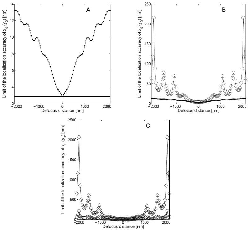
The figure shows the behavior of the limit of the localization accuracy of the x₀ (y₀) coordinate of a single-molecule/point-source as a function of defocus distance. Panel A shows the fundamental limit of the 3D localization accuracy ${\delta }_{x_0}^{3d}$ that is given in eq. 8 (●). The fundamental limit of the 2D localization accuracy ${\delta }_{x_0}^{2d}$ that is given in eq. 10 is also shown for reference (—). Panel B shows the limit of the 3D localization accuracy for x₀ (y₀) for a pixelated detector in the absence of noise sources (○), and panel C shows the same in the presence of noise sources (◇). Panels B and C also show the 3D fundamental limit ${\delta }_{x_0}^{3d}$ (●) and the limit of the 3D localization accuracy of z₀ in the absence of noise sources (○), respectively for reference. In all the plots the photon detection rate is set to be Λ₀ = 5000 photons/s, the acquisition time is set to be t = 0.1 s (with t₀ = 0), the numerical aperture is set to be NA = 1.3, the magnification is set to be M = 100, the wavelength of the detected photons from the single molecule is set to be λ = 520 nm, the pixel array size is set to be 5 × 5, the pixel size is set to be 13μm × 13μm, the mean of the Poisson noise component is set to be β(k, t) = 25 photons/pixel, and the mean and the standard deviation of the Gaussian noise component are set to be η_k = 0 and σ_w,k = 8e⁻ rms, respectively. The noise statistics are assumed to be the same for all the pixels and the image of the single molecule is assumed to be centered on the pixel array.

Figure 3A shows the behavior of the fundamental limit of the 3D localization accuracy ${\delta }_{z_0}^{3d}$ of the z₀ coordinate as a function of z₀. Unlike ${\delta }_{x_0}^{3d}$ the 3D fundamental limit ${\delta }_{z_0}^{3d}$ becomes infinitely large as z₀ approaches zero. From eq. 9, we see that the term (∂q_z0(x, y)/∂z₀) appears in the denominator of the expression for the fundamental limit ${\delta }_{z_0}^{3d}$. Further, for the phase aberration term W_z0 given in eq. 11, it can be shown that as z₀ approaches 0, (∂q_z0(x, y)/∂z₀) tends to 0 for every (x, y) ∈ ℝ² (see eq. 7), thereby explaining the observed behavior of ${\delta }_{z_0}^{3d}$ at z₀ = 0. As z₀ increases (decreases), ${\delta }_{z_0}^{3d}$first decreases but then increases monotonically up to z₀ = ±1000 nm. For z₀ values greater (smaller) than 1000 nm (-1000 nm), ${\delta }_{z_0}^{3d}$ deteriorates with an oscillatory behavior, which is analogous to the behavior of the 3D fundamental limit of the x₀ coordinate. Note that here also the behavior of ${\delta }_{z_0}^{3d}$ is symmetric about z₀ = 0.

Figure 3.

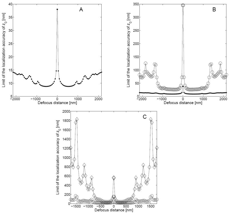
The figure shows the behavior of the limit of the localization accuracy of the z₀ coordinate of a single-molecule/point-source as a function of defocus distance. Panel A shows the fundamental limit of the 3D localization accuracy (●) ${\delta }_{z_0}^{3d}$ that is given in eq. 9. Panel B shows the limit of the 3D localization accuracy for z₀ for a pixelated detector in the absence of noise sources (○), and panel C shows the same in the presence of noise sources (◇). Panels B and C also show the 3D fundamental limit ${\delta }_{z_0}^{3d}$ (●) and the limit of the 3D localization accuracy of z₀ in the absence of noise z₀ sources (○), respectively for reference. Note that unlike the x₀ coordinate (see Fig. 2), the limit of the 3D localization accuracy for the z₀ coordinate becomes infinitely large as the defocus distance approaches zero. The numerical values for generating the above plots are identical to those used in Fig. 2.

3. EFFECTS OF PIXELATION AND NOISE SOURCES

In deriving the fundamental limit of the localization accuracy, we assumed that the acquired data consists of the time points and the spatial coordinates of the detected photons. However, current imaging detectors contain (finite sized) pixels and the acquired data consists of the number of detected photons at each pixel. For a pixelated detector {C₁,…,C_Np} the number of detected photons (from the single molecule) at the k^th pixel C_k can be shown¹⁸ to be independently Poisson distributed with mean ${\mu }_{\theta }\left(k,t\right)={\mathit{\int }}_{t_0}^t{\mathit{\int }}_{C_k}{\mathrm{\Lambda }}_{\theta }\left(\tau \right)f_{\theta }\left(r\right)d\tau \mathit{dr},\theta \in \mathrm{\Theta }$, k = 1,…,N_p. Here we make no assumptions about the specific shape, size or orientation of the pixels. We only assume that the pixels do not overlap. We consider two additive noise sources, namely Poisson and Gaussian noise sources, which are commonly encountered in experimental data. Poisson noise is used to model the effect of scattered photons, which, for example, arise due to cellular autofluorescence and scattering. Gaussian noise is used to model the effect of measurement noise, which, for example, arises during the readout process in the detector. Therefore the acquired data in a pixelated detector can be modeled as a sequence {I_θ,1,…,I_θ, N_p} random variables given by

$$I_{\theta ,k}=S_{\theta ,k}+B_k+W_k,k=1,\mathrm{...},N_p,\theta \in \mathrm{\Theta },$$

where S_θ,k (B_k) is an independent Poisson random variable with mean μ_θ(k, t) (β(k, t)) and W_k Gaussian random variable with mean η_k and variance ${\sigma }_{w,k}^2$, k = 1,…,N_p. We assume that {S_θ,1,…,S_θ,Np}, {B₁,…,B_Np} and {W₁,…,W_Np} are mutually independent, and that β(k, t), η_k and σ_w,k are independent of θ, k = 1,…,N_p.

In the absence of noise sources, the Fisher information matrix for the data acquired in a pixelated detector during the fixed time interval [t₀, t] is given by¹⁸

$$\mathbf{I}(\theta )={\sum _{k=1}^{N_p}\left(\frac{\partial {\mu }_{\theta }(k,t)}{\partial \theta }\right)}^T\frac{\partial {\mu }_{\theta }(k,t)}{\partial \theta },\theta \in \mathrm{\Theta },$$

where μ_θ is defined above,

$$\frac{\partial {\mu }_{\theta }(k,t)}{\partial \theta }:={\left[\begin{array}{l}{\mathit{\int }}_{t_0}^t{\mathit{\int }}_{C_k}{\mathrm{\Lambda }}_{\theta }(\tau )\frac{\partial f_{\theta }(r)}{\partial x}\mathit{drd}\tau \\ {\mathit{\int }}_{t_0}^t{\mathit{\int }}_{C_k}{\mathrm{\Lambda }}_{\theta }(\tau )\frac{\partial f_{\theta }(r)}{\partial y}\mathit{drd}\tau \\ {\mathit{\int }}_{t_0}^t{\mathit{\int }}_{C_k}{\mathrm{\Lambda }}_{\theta }(\tau )\frac{\partial f_{\theta }(r)}{\partial z_0}\mathit{drd}\tau \\ {\mathit{\int }}_{t_0}^t{\mathit{\int }}_{C_k}\frac{\partial {\mathrm{\Lambda }}_{\theta }(\tau )}{\partial {\mathrm{\Lambda }}_0}{f}_{\theta }(r)\mathit{drd}\tau \end{array}\right]}^T,k=1,\mathrm{...},N_p,\theta =(x_0,y_0,z_0,{\mathrm{\Lambda }}_0)\in \mathrm{\Theta },$$ (12)

and f_θ is given in eq. 1 with q_z0 given by eq. 3. Here also we assume that the phase aberration term is given by eq. 11. In the presence of both Poisson and Gaussian noise, the Fisher information matrix for the data acquired in a pixelated detector during the fixed time interval [t₀, t] is given by¹⁸

$$\mathbf{I}(\theta )=\sum _{k=1}^{N_p}{\left(\frac{\partial {\mu }_{\theta }(k,t)}{\partial \theta }\right)}^T\frac{\partial {\mu }_{\theta }(k,t)}{\partial \theta }\left({{\mathit{\int }}_{ℝ}\frac{\left({\sum }_{l=1}^{\infty }\frac{{[{\nu }_{\theta }(k,t)]}^{l-1}{e}^{-{\nu }_{\theta }(k,t)}}{\left(l-1\right)!}\cdot \frac{1}{\sqrt{2\pi }{\sigma }_{w,k}}{e}^{-\frac{1}{2}{\left(\frac{z-l-{\eta }_k}{{\sigma }_{w,k}}\right)}^2}\right)}{p_{\theta ,k}(z)}}^{2}dz-1\right),\theta \in \mathrm{\Theta },$$

where ∂μ_θ(k,t)/∂θ is given by eq. 12, ν_θ(k,t) := μ_θ(k,t) + β(k,t), k = 1,…,N_p and

$$p_{\theta ,k}(z):=\frac{1}{\sqrt{2\pi }{\sigma }_{w,k}}\sum _{l=0}^{\infty }\frac{{[{\nu }_{\theta }(k,t)]}^l{e}^{-{\nu }_{\theta }(k,t)}}{l!}{e}^{-\frac{1}{2}{\left(\frac{z-l-{\eta }_k}{{\sigma }_{w,k}}\right)}^2},z\in ℝ,k=1,\mathrm{...},N_p.$$

To calculate the limit of the 3D localization accuracy in the presence/absence of noise for a pixelated finite detector, we invert the corresponding Fisher information matrix I(θ) and take the square root of the appropriate term in the main diagonal.

Fig. 2B (Fig. 3B) shows the behavior of the limit of the 3D localization accuracy of the x₀/y₀ (z₀) coordinate for a pixelated finite detector in the absence of noise sources. From the figure we see that the limit of the 3D localization accuracy of x₀ (z₀) exhibits a behavior that is analogous to the fundamental limit ${\delta }_{x_0}^{3d}$( ${\delta }_{z_0}^{3d}$). Note that the limit of the 3D localization accuracy of x₀ (z₀) for the pixelated finite detector is greater than the fundamental limit ${\delta }_{x_0}^{3d}$( ${\delta }_{z_0}^{3d}$) for all values of the defocus distance. This can be explained by noting that in a pixelated finite detector, due to its finite size, not all the photons that reach the detector plane are detected (see Fig. 1), and that the spatial coordinates of the detected photons are known only up to a pixel. Note that for large defocus distances, the oscillatory behavior of the limit of the 3D localization accuracy for a pixelated detector becomes prominent when compared to the fundamental limit.

Fig. 2C (Fig. 3C) shows the dramatic effect of noise on the behavior of the limit of the 3D localization accuracy of the x₀/y₀ (z₀) coordinate for a pixelated finite detector. We see that the limit of the 3D localization accuracy in the presence of noise shows significant deterioration when compared to the noise free case, especially for defocus distances greater (smaller) than 1 μm (−1 μ m). Note that in the presence of noise, the oscillatory behavior of the limit of the 3D localization accuracy also becomes more pronounced, when compared to the noise free case.

The results presented in this paper provide insight into the extent to which single molecules can be accurately tracked in three dimensions. Since these results provide a limit to the localization accuracy, they can be used as a benchmark to compare the performance of different algorithms that are used to estimate the 3D location of a single molecule from experimental data. The present results can be used in several ways in the context of single molecule microscopy, such as in the design of an experimental setup for tracking single molecules.

References

- 1.Moerner WE, Fromm DP. Methods of single-molecule fluorescence spectroscopy and microscopy. Rev Sci Instrum. 2003;74(8):3597–3619. [Google Scholar]
- 2.Weiss S. Fluorescence spectroscopy of single biomolecules. Science. 1999;283:1676–1683. doi: 10.1126/science.283.5408.1676. [DOI] [PubMed] [Google Scholar]
- 3.Schütz GJ, Axmann M, Schindler H. Imaging single molecules in three dimensions. Sing Mol. 2001;2(2):69–74. [Google Scholar]
- 4.Zacks S. The theory of statistical inference. John Wiley and Sons; New York, USA: 1971. [Google Scholar]
- 5.Kay SM. Fundamentals of statistical signal processing. Prentice Hall PTR; New Jersey, USA: 1993. [Google Scholar]
- 6.Bartko AP, Dickson RM. Three-dimensional orientations of polymer-bound single molecules. J Phys Chem B. 1999;103(16):3053–3056. [Google Scholar]
- 7.Bartko AP, Dickson RM. Imaging three-dimensional single molecule orientations. J Phys Chem B. 1999;103(51):11237–11241. [Google Scholar]
- 8.Schutz GJ, Pastushenko VP, Gruber HJ, Knaus HG, Pragl B, Schindler H. 3D imaging of individual ion channels in live cells at 40 nm resolution. Sing Mol. 2000;1(1):25–31. [Google Scholar]
- 9.Subotic N, DeVille DV, Unser M. On the feasibility of axial tracking of a fluorescent nano-particle using a defocussing model. Proc IEEE Intl Conf Biomedical Imaging: From Macro to Nano. 2004:1231–1234. [Google Scholar]
- 10.Snyder DL, Helstrom CW, Lanterman AD, White RL. Compensation for read out noise in charge coupled device images. J Opt Soc Am A. 1995;12(2):272–283. [Google Scholar]
- 11.Ober RJ, Ram S, Ward ES. Localization accuracy in single molecule microscopy. Biophys J. 2004;86:1185–1200. doi: 10.1016/S0006-3495(04)74193-4. [DOI] [PMC free article] [PubMed] [Google Scholar]
- 12.Saleh B. Photoelectron statistics. Springer Verlag; Berlin, Germany: 1978. [Google Scholar]
- 13.Snyder DL, Miller MI. Random point processes in time and space. 2. Springer Verlag; New York, USA: 1991. [Google Scholar]
- 14.Gibson SF. PhD thesis. Carnegie-Mellon University; 1990. Modelling the 3D imaging properties of the fluorescence light microscope. [Google Scholar]
- 15.Gibson SF, Lanni F. Diffraction by a cirular aperture as a model for three-dimensional optical microscopy. J opt soc Am A. 1989;6(9):1357–1367. doi: 10.1364/josaa.6.001357. [DOI] [PubMed] [Google Scholar]
- 16.Gibson SF, Lanni F. Experimental test of an analytical model of aberration in an oil-immersion objective lens used in three-dimensional light microscopy. J opt soc Am A. 1992;9(1):154–166. doi: 10.1364/josaa.9.000154. [DOI] [PubMed] [Google Scholar]
- 17.Born M, Wolf E. Principles of Optics. Cambridge University Press; Cambridge, UK: 1999. [Google Scholar]
- 18.Ram S, Ward ES, Ober RJ. A stochastic analysis of performance limits for optical microscopes. submitted. [Google Scholar]