A LAGUERRE VORONOI BASED SCHEME FOR MESHING PARTICLE SYSTEMS

Abstract

We present Laguerre Voronoi based subdivision algorithms for the quadrilateral and hexahedral meshing of particle systems within a bounded region in two and three dimensions, respectively. Particles are smooth functions over circular or spherical domains. The algorithm first breaks the bounded region containing the particles into Voronoi cells that are then subsequently decomposed into an initial quadrilateral or an initial hexahedral scaffold conforming to individual particles. The scaffolds are subsequently refined via applications of recursive subdivision (splitting and averaging rules). Our choice of averaging rules yield a particle conforming quadrilateral/hexahedral mesh, of good quality, along with being smooth and differentiable in the limit. Extensions of the basic scheme to dynamic re-meshing in the case of addition, deletion, and moving particles are also discussed. Motivating applications of the use of these static and dynamic meshes for particle systems include the mechanics of epoxy/glass composite materials, bio-molecular force field calculations, and gas hydrodynamics simulations in cosmology

1. INTRODUCTION

Particles are smooth functions with compact support. Particle systems are used for modeling a number of physical world scenarios ranging from cosmological systems and plasma physics to molecular systems. The applications are wide and varied and include chemistry, material science, and bio-engineering. A typical astrophysics computation attempts to follow the evolution of a system of cosmological boundaries, modeled as a particle system. An important computation performed on the particle system is that of force calculations, i.e. given n particles compute the effect of the gravitational or hydrodynamic force on a given particle by the other particles. These are often termed as n-body problems. Other characteristics of the problem require tracking the dynamic structure of the particle system as particle systems move, appear and disappear.

Smooth particle hydrodynamics or SPH [1] is a Lagrangian numerical hydrodynamics method that uses a discrete description of gas or fluid particles in place of a continuum model. The value of a field at a point in space is given by the sum of any contributing particles, and their radially symmetric kernels, present at that point. These particles essentially act as moving centers for interpolation and carry mass, energy and the velocity of the local flow. For the meshing of particle systems, it suffices to consider particles as idealized balls, or radially symmetric domains of support of their kernels. So henceforth, we consider our particle systems to be a collection of circles in two dimensions, and spheres in three dimensions, with possibly different radii.

Main Contributions

We present Laguerre Voronoi based subdivision algorithms for the quadrilateral and hexahedral meshing of particle systems within a bounded region, for two and three dimensions, respectively. Extensions of the basic scheme to dynamic re-meshing in the case of addition, deletion, and moving particles are also discussed.

Applications

A motivating application for finite element mesh constructions of a static particle system is for the accurate calculation of stress distributions for composite materials consisting of silica substrates with embedded particles, subjected to various loads [2]. The re-meshing problem for time dependent particle systems arise in gas hydrodynamics simulations essential in the computational investigation of the formation of large scale structures, such as galaxies and galaxy clusters, in the universe [3]. A third motivating application domain is the use of finite element meshes of particle systems for biophysics simulations of molecular interactions in ionic solvent [4].

Prior Related Work

Laguerre Voronoi diagrams [5, 6, 7] or its variants like STC [8], embedded Voronoi Graphs [9], [10], or medial surfaces [11] have been extensively used to generate hexahedral meshes. A variant of the Voronoi diagram called the Space Twist Continuum (STC) [8] has also been successfully used at the Sandia Labs in their meshing software CUBIT. STC is a way of representing the dual of the hexahedral mesh as a simple non-degenerate arrangement of surfaces. The STC is built in an incremental fashion using an Advancing Front Techniques (AFT) like the Whisker Weaving algorithm [8].

As reviewed in [12] [13], there are indirect and direct methods for unstructured quad/hex mesh generation. The indirect method is to generate triangular/tetrahedral meshes first, then convert them into quads/hexes. The direct method is to generate quads/hexes directly without first going through triangular/tetrahedral meshing [14]. Alternatively, Pascal et al give an overview of the grid based approaches for Hexahedral meshing [15]. Either higher order elements can be used to represent the exact boundary of the surface by intersecting it with the grid, or body-fitting techniques can be used to represent these boundary elements [16], [17]. Dual contouring has also been used by Zhang et al [18], [19], for extracting hexahedral meshes from volumetric data.

Subdivision defines a smooth curve or surface as the limit of a sequence of successive refinements of some linear input [20]. As a structured method, quad/hex mapped meshing [21] generates the most desirable meshes if opposite edges/faces of the domain to be meshed have equal numbers of divisions or the same surface mesh. However, it is always difficult to decompose an arbitrary geometric configuration into mapped meshable regions. In the CUBIT project [22] at Sandia National Labs, several techniques have been attempted to automatically recognize features and decompose geometry into mapped meshable areas or volumes.

The simplest method for post mesh quality improvement is based on Laplacian smoothing which relocates the vertex position at the average of the nodes connecting to it [23]. Optimization-based smoothing tends to yield better results but it is more expensive than Laplacian smoothing [24], [25], [26]

2. QUADRILATERAL MESHING

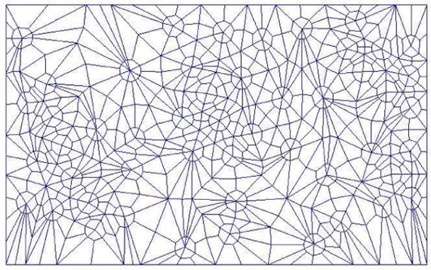
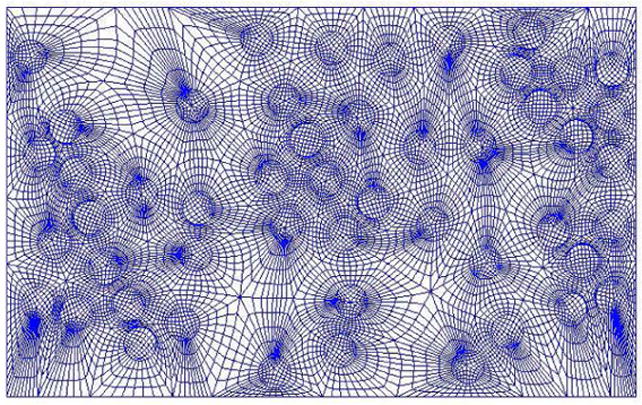
Two dimensional particles are circles of possibly different radii. A typical input particle system along with its output conforming quadrilateral mesh, inside a rectangular bounding box, is shown in Figure 1.

Figure 1.

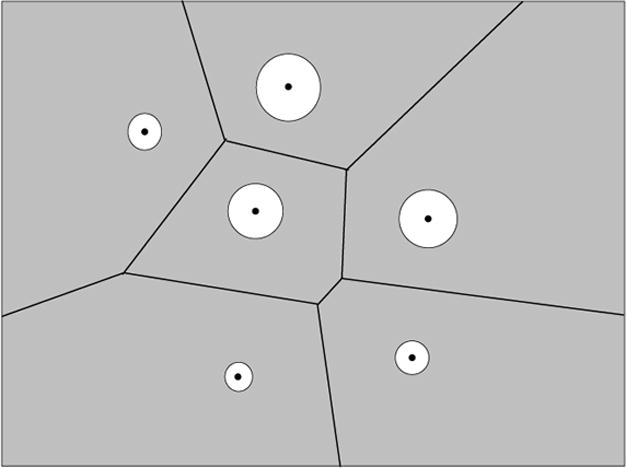
Tesselating the initial bounding region by Laguerre Voronoi cells.

Step 1

Construct the 2D Laguerre Voronoi diagram of the center points of the circles within its rectangular bounding region (see figure 1). The weight of a circle center is chosen to be proportional to the radius of each circle. Each Voronoi cell is a convex polygon.

Step 2

Contract the short edges into either of its endpoint vertices, or to the center point of the edge, unless boundary constraints as mentioned below are violated (see figure 2). An edge is regarded as short if its length is less than a user specified threshold value.

Figure 2.

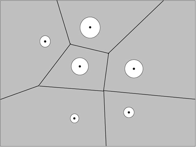
Simplification of the Laguerre Voronoi diagram by contracting small edges

Note that this edge contraction may eliminate triangles (see figure 3). The aim of this small edge contraction step is to avoid producing tiny quadrilateral elements. Also note that if an edge contraction causes an intersection between the boundaries of a polygonal cell and the circle perimeter, then we do not carry out this edge contraction.

Figure 3.

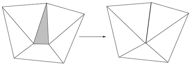
Contracting an edge sometime leads to the contraction of a triangle

Step 3

For each Voronoi cell, connect the circle center with the vertices, and the midpoint of each Voronoi cell edge. Partially delete the inner portion (i.e. within each circle) of the line segment that connects the circle center to the midpoint of each Voronoi edge, thereby creating quadrilaterals both inside and outside each circle, i.e. a quad tesselation. (see figures 5 and 6).

Figure 5.

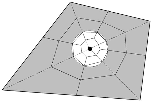
Partitioning of the Laguerre Voronoi Diagram into Quadrilaterals

Figure 6.

Further partitioning of the Laguerre Voronoi Diagram yields a quad tesselation of the bounding region for the particle system

Step 4

Next, further refinement of the quad tesselation is accomplished by first a quad mesh splitting along the radial and angular directions from each circle center, followed by an averaging/smoothing recalculation [27] to place all quad mesh vertices (see figure 7). Note the selective splitting of the inner most radial edges from each circle center, to preserve quad mesh topology (see figures 8. The aim of the splitting step is to achieve quad mesh adaptivity.

Figure 7.

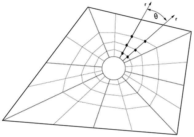
The quadrilateral mesh after a radial/angular quad subdivision step outside to the particles

Figure 8.

The quadrilateral mesh after a quad subdivision step inside/outside the particles.

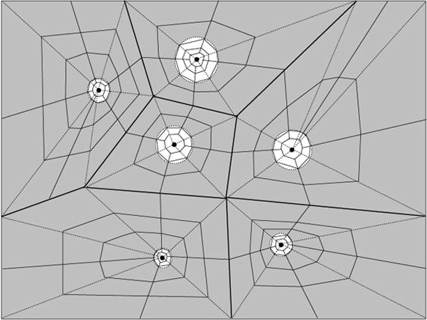
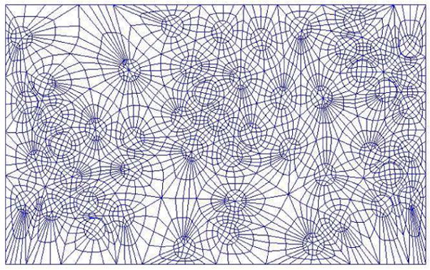
The averaging/smoothing based repositioning of the mesh vertices can be carried out, in a variety of ways. We choose to adopt a centroid smoothing scheme, where each vertex is repositioned in the centroid of the centroids of the maximal dimensional cells incident to it (taking care of boundary vertices as well) [27]. While we do not have a guarantee for mesh quality, the current averaging scheme tends to produce quads with very good aspect ratio. See figures 9,10,11,12 for examples of our implementation of this algorithm.

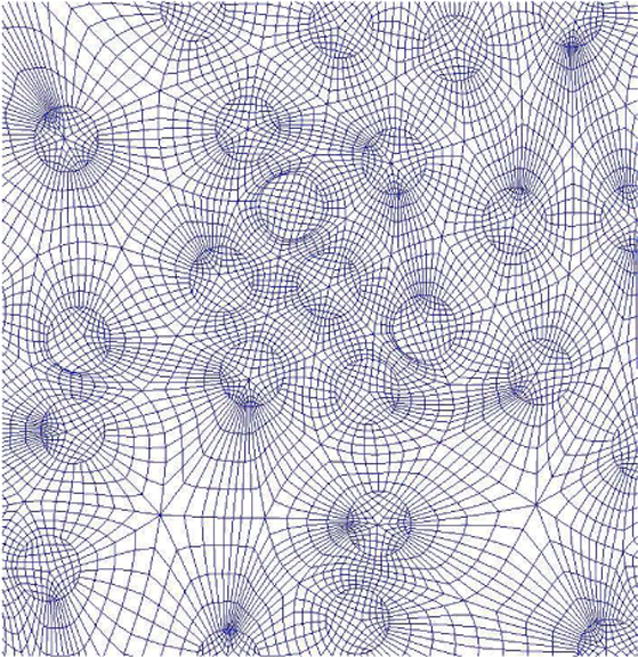
Figure 9.

The quadrilateral mesh after recursive quad subdivision refinement

Figure 10.

The quadrilateral mesh after several steps of subdvision refinement

Figure 11.

Zoomed in view of the mesh shown in figure 10.

Figure 12.

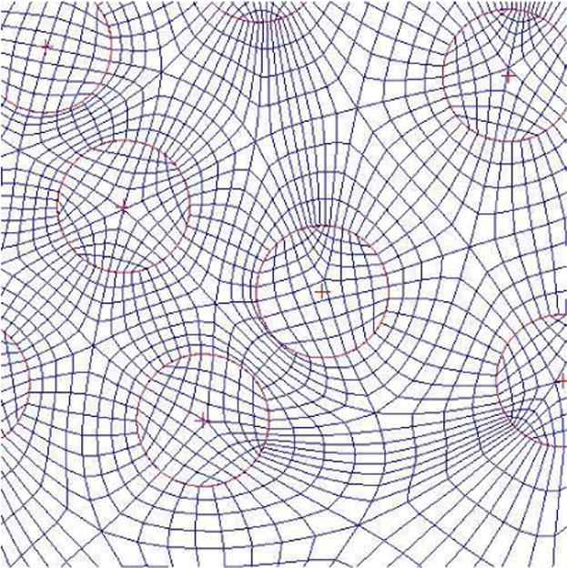
Zoomed in view of the mesh shown in figures 10 and 11.

3. HEXAHEDRAL MESHING

In this section we present the solution in three dimensions.

Step 1

Construct the 3D weighted Voronoi diagram of the center points the spheres (see figure 13). The weight of a sphere center is chosen to be proportional to the radius of the sphere.

Figure 13.

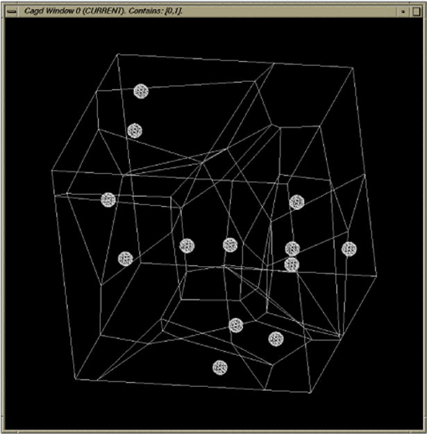
Tesselating the initial bounding region by Laguerre Voronoi cells. Each cell is a convex polyhedron in 3D.

Step 2

Contract each of the short edges into single vertices. An edge is regarded as short if its length is less than a user specified threshold value. Note that this contraction may eliminate triangles (see Fig 3). Also note that this merging may lead to the intersection between the boundaries of polyhedral cells and the surface of the sphere, and so a check is made, and such edge contractions are not carried out. The aim of this step is to avoid producing very tiny hexahedral elements.

Step 3

Decompose each face of the 3D Voronoi cells into quads (see Fig 14). For each Laguerre Voronoi cell, connect the particle center with the Voronoi vertices and thereby form a pyramidal partition of the cell. Each pyramid is further split into a hexahedron and another pyramid by a quad face generated by intersection with the surface of the sphere.

Figure 14.

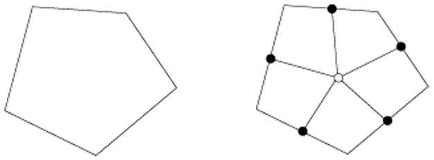
Subdivision of the face polygon of Voronoi cells into quadrilaterals. The empty dot is the centroid of the polygon. The darkened dots are the mid-points of the edges.

Step 4

Adaptive subdivision of each cell is easily performed in the radial direction (see figure 15).

Figure 15.

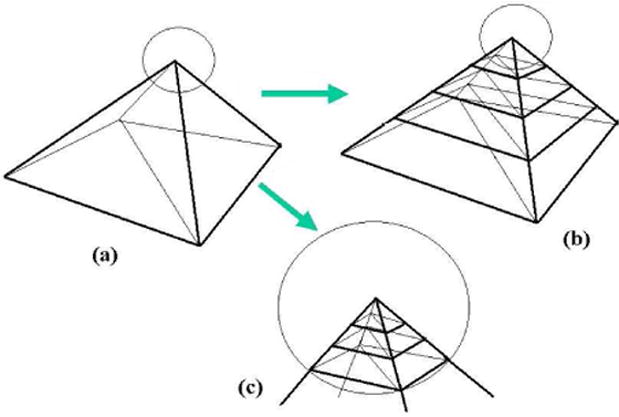
Adaptive subdivision in the radial direction.

At this stage one has almost obtained a complete adaptive hexahedral mesh of the bounding region, conforming to the boundary of the particle spheres. The mesh elements incident to the particle centers are quad pyramids, while the rest of the mesh elements are hexahedra. By repeated applications of the radial subdivision, the pyramidal elements can be restricted to very small spheres surrounding each particle center. In many applications, where calculations are desired close to the surface of the particle spheres, or only on its exterior, this near hexahedral mesh suffices. See also figure 16 of an example mesh generated for a small portion of a heterogenous elastic material with spherical inclusions with different bulk properties to the rest of the substrate.

Figure 16.

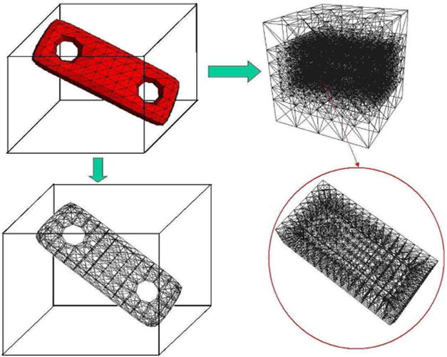
Hexahedral meshing of a portion of a heterogeneous composite material with glass sphere inside an epoxy substrate

Step 5

Further improve the hexahedral mesh quality, by applying the averaging/smoothing based repositioning of the mesh vertices using the centroid smoothing scheme of [27], which tends to produce hexahedra with good aspect ratio. This averaging/smoothing can also be conducted with varied crease rules, to produce user desired mesh anisotropy.

N.B. A current disadvantage of the centroid smoothing scheme [27] that we use for mesh quality improvement, is the lack of a guarantee of producing “good” (e.g. bounded aspect ratio, positive Poisson ratio) meshes. Furthermore, in three dimensions there is the occasional failure to maintain convexity of the subsequently partitioned hexahedra after several iterations of averaging/smoothing. While in our current implementation, we do not perform the step that causes “bad” hexahedra, we are currently working on an improved weighted averaging/smoothing scheme for hexahedral mesh quality improvement.

Alternate Step

In the case where a complete hexahedral element mesh is required both inside and outside the spheres, one can use the following alternate hexahedral scaffolding scheme. First, split each face of the Voronoi cell into triangles. Next connect each vertex of the triangulated Voronoi faces to the center of their respective particle centers, decomposing the entire bounding region into tetrahedra. The tetrahedra are further decomposed by the (piecewise linear) surfaces of the particle spheres into triangular prisms, and tetrahedra incident to the center of the particles. Each triangular prism can be split into 3 hexahedra and the tetrahedra at the particle centers, are split into four hexahedra by adding three vertices on the edges and one vertex on the face (see figures 17 and 18). After this step, the entire bounding region, with the particle system, is partitioned into hexahedra.

Figure 17.

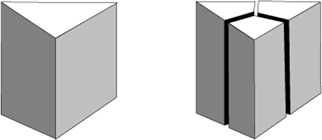
Splitting of a triangular prism into 3 hexahedra

Figure 18.

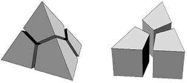
Splitting a tetrahedron into four hexahedra. The right image only displays three of the hexahedra, with the fourth hexahedron (top) omitted for visual clarity

Features of the Constructed Mesh

The hexahedral mesh constructed is adaptive in the sense that it becomes denser in the regions that are close to the surfaces of the sphere. When averaging/smoothing (recursive subdivision) rules are used, the mesh is uniform in the sense that at the regions which are the same distance to a sphere, the elements are similar to each other. See figures 19, 20.

Figure 19.

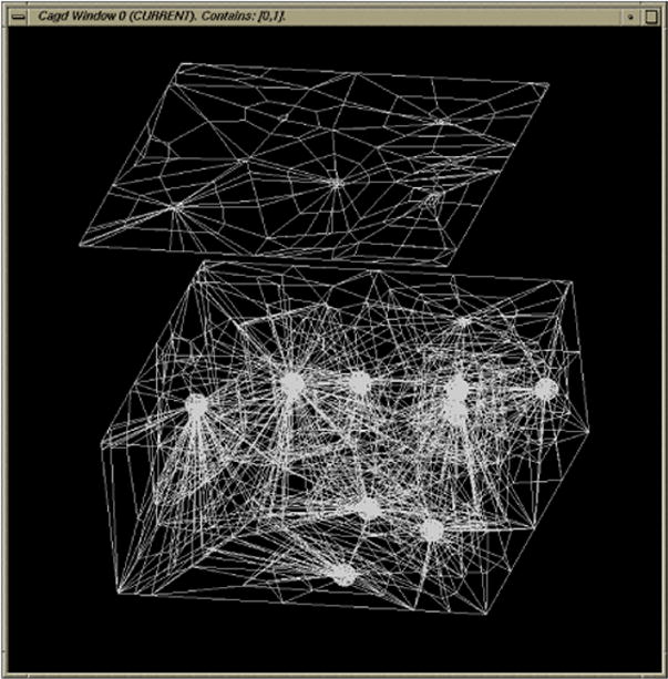
The hexahedral mesh after a couple of steps of our adaptive hexahedral recursive subdivision refinement

Figure 20.

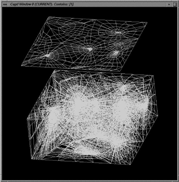
The hexahedral mesh after a further steps of our adaptive hexahedral recursive subdivision refinement

4. EXTENSIONS TO DYNAMIC PARTICLE SYSTEMS

Our extensions to the re-meshing of dynamic particle systems is based on dynamic Laguerre Voronoi diagrams. The partitioning and recursive subdivision follows directly from the instantaneous position of the particle system and its Voronoi diagram. Dynamic Voronoi diagrams have been well studied [28, 29, 30, 31, 32, 33, 34, 35]. Dynamic Laguerre Voronoi diagrams have also been considered [36, 37].

5. CONCLUDING REMARKS

We have incorporated our quadrilateral and hexahedral meshing schemes to two and three dimensional stress/strain finite element simulations involving epoxy/glass composite materials under static and dynamic loading scenarios in computational mechanics [2]. We are currently also using this mesher to develop a fast non-uniform fast-Fourier transform based n-body gravitational force calculation, coupled to smooth particle gas hydrodynamics simulations in computational cosmology [3]. Further, we hope to apply extensions of this scheme to Poisson-Boltzmann and Smoluchowski equations [4] as well as additional biophysics simulations.

Figure 4.

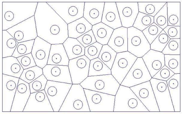
A Simplified Voronoi Diagram for a Particle System in a rectangular bounded region

References

- 1.Gingold R, Monaghan J. Smoothed particle hydrodynamics: theory and application to non-spherical stars. Royal Astronomical Society. 1977;181:375–389. [Google Scholar]
- 2.Vemaganti K, Oden T. Estimation of Local Modeling Error and Goal-Oriented Adaptive Modeling of Heterogeneous Materials, Part II: A Computational Environment for Adaptive Modeling of Heterogeneous Elastic Solids. Computer Methods Appl Mechanical Engineering. 2001:6089–6124. [Google Scholar]
- 3.Hockney RW, Eastwood JW. Computer Simulation Using Particles. McGraw-Hill; 1981. [Google Scholar]
- 4.Song Y, Zhang Y, Shen T, Bajaj CL, McCammon JA, Baker NA. Finite element solution of the steady-state Smoluchowski equation for rate constant calculations. Biophysical Journal. 2004;86(4):1–13. doi: 10.1016/S0006-3495(04)74263-0. [DOI] [PMC free article] [PubMed] [Google Scholar]
- 5.Imai H, Iri M, Murota K. Voronoi Diagram in the Laguerre Geometry and Its Applications. SIAM Journal on Computing. 1985;1 [Google Scholar]
- 6.Berg MD, Kreveld MV, Overmars M, Schwarzkopf O, Kreveld MV. Computational Geometry. Springer Verlag; 2000. [Google Scholar]
- 7.Okabe A, Boots B, Sugihara K. Spatial Tessellations: Concepts and Applications of Voronoi Diagrams. John Wiley and Sons; 1992. [Google Scholar]
- 8.Tautges TJ, Blacker TD, Mitchell SA. The Whisker Weaving Algorithm: A Connectivity Based Method for Constructing All Hexahedral Finite Element Meshes. International Journal of Numerical Methods in England. 1996;39 [Google Scholar]
- 9.Sheffer A, Etalon M, Rapports A, Beckoner M. Hexahedral Mesh Generation using the Embedded Voronoi Graph. Proceedings, 7th International Meshing Roundtable, Sandia National Labs; 1998. pp. 347–364. [Google Scholar]
- 10.Li TS, McKeag R, Armstrong CG. Hexahedral Meshing using Midpoint Subdivision and Integer Programming. Computer Methods in Applied Mechanics and Engineering. 1995;124:171–193. [Google Scholar]
- 11.Price M, Armstrong C. Hexahedral mesh generation by medial surface subdivision: Part I. Int J Numer Meth Engng. 1995;38(19):3335–3359. [Google Scholar]
- 12.Owen S. A survey of unstructured mesh generation technology. 7th International Meshing Roundtable; 1998. pp. 26–28. [Google Scholar]
- 13.Teng SH, Wong CW. Unstructured mesh generation: Theory, practice, and perspectives. International Journal of Computational Geometry and Applications. 2000;10(3):227–266. [Google Scholar]
- 14.Eppstein D. Linear Complexity Hexahedral Mesh Generation. Symposium on Computational Geometry; 1996. pp. 58–67. [Google Scholar]
- 15.Pascal JF, George PL. Mesh Generation. Hermes Science Publishing; 2000. [Google Scholar]
- 16.Schneiders R, Schindler R, Weiler F. Octree-Based Generation of Hexahedral Element Meshes. 5th International Meshing Roundtable, Sandia National Labs; 1996. pp. 205–216. [Google Scholar]
- 17.Wada Y. Effective Adaptation Technique for Hexahedral Mesh. Concurrency and Computation: Practice and Experience. 2002;14:451–463. [Google Scholar]
- 18.Zhang Y, Bajaj C, Sohn B. Adaptive and Quality 3D Meshing from Imaging Data. 8th ACM Symposium on Solid Modeling and Applications; 2003. pp. 286–291. [Google Scholar]
- 19.Zhang Y, Bajaj C, Sohn BS. 3D Finite Element Meshing from Imaging Data. To appear in the special issue of Computer Methods in Applied Mechanics and Engineering (CMAME) on Unstructured Mesh Generation . 2004 doi: 10.1016/j.cma.2004.11.026. www.ices.utexas.edu/~jessica/meshing. [DOI] [PMC free article] [PubMed]
- 20.Schroder P, Zorin D, DeRose T, Kobbelt L, Stam J, Warren J. Subdivision for Modeling and Animation. Siggraph; 1999. Special course notes. [Google Scholar]
- 21.Cook WA, Oakes WR. Mapping methods for generating three-dimensional meshes. Computers in Mechanical Engineering. 1982:67–72. [Google Scholar]
- 22.CUBIT Mesh Generation Toolkit. Web site: http://sass1693.sandia.gov/cubit.
- 23.Field D. Laplacian smoothing and Delaunay triangulations. Communications in Applied Numerical Methods. 1988;4:709–712. [Google Scholar]
- 24.Canann S, Tristano J, Staten M. An approach to combined Laplacian and optimization-based smoothing for triangular, quadrilateral and quad-dominant meshes. 7th International Meshing Roundtable; 1998. pp. 479–494. [Google Scholar]
- 25.Freitag L. On combining Laplacian and optimization-based mesh smoothing techniques. AMD-Vol 220 Trends in Unstructured Mesh Generation. 1997:37–43. [Google Scholar]
- 26.Freitag L, Ollivier-Gooch C. Tetrahedral mesh improvement using swapping and smoothing. Int J Numer Meth Engng. 1997;40:3979–4002. [Google Scholar]
- 27.Bajaj C, Schaeffer S, Warren J, Xu G. A Subdivision Scheme for Hexahedral Meshes. The Visual Computer. 2002;18(5–6):343–356. [Google Scholar]
- 28.Bajaj CL, Bouma WJ. Dynamic Voronoi diagrams and Delaunay triangulations. Proc. 2nd Canadian Conference on Computational Geometry; 1990. pp. 273–277. [Google Scholar]
- 29.Imai H, Iri M, Murota K. Voronoi Diagram In the Laguerre Geometry and its Applications. SIAM Journal of Computing. 1985;14:93–10. [Google Scholar]
- 30.Chew P. Near-Quadratic Bounds for the L1 Voronoi Diagram of Moving Points. Computational Geometry Theory and Applications. 1997;7 [Google Scholar]
- 31.Fu JJ, Lee RCT. Voronoi Diagrams of Moving Points in the Plane. International Journal of Computational Geometry and Applications. 1991;1(1):23–32. [Google Scholar]
- 32.Guibas L, Mitchell JSB, Roos T. Voronoi Diagrams of Moving Points in the Plane. Proc. 17th Internat. Workshop Graph-Theoret. Concepts Comput. Sci., vol. 570 of Lecture Notes in Computer Science; Springer-Verlag; 1991. pp. 113–125. [Google Scholar]
- 33.Albers G, Roos T. Voronoi Diagrams of Moving Points in Higher Dimensional Spaces. Proc. 3rd Scand. Workshop Algorithm Theory, vol. 621 of Lecture Notes in Computer Science; Springer-Verlag; 1992. pp. 399–409. [Google Scholar]
- 34.Roos T. Voronoĭ Diagrams over Dynamic Scenes. Discrete Applied Mathematics. Combinatorial Algorithms, Optimization and Computer Science. 1993;43(3):243–259. [Google Scholar]
- 35.Roos T. New Upper Bounds on Voronoi Diagrams of Moving Points. Nordic Journal of Computing. 1997;4(2):167–171. [Google Scholar]
- 36.Imai K, Imai H. On Weighted Dynamic Voronoi Diagrams. In: Avis D, Bose P, editors. Snapshots of Computational and Discrete Geometry. Vol. 3. 1994. pp. 268–277. [Google Scholar]
- 37.Anton F, Mioc D. Dynamic Laguerre Diagrams Made Easy. European Workshop on Computational Geometry; 2000. pp. 10–13. [Google Scholar]