Measuring Aptamer Equilbria Using Gradient Micro Free Flow Electrophoresis

Abstract

Gradient micro free flow electrophoresis (μFFE) was used to observe the equilibria of DNA aptamers with their targets (IgE or HIVRT) across a range of ligand concentrations. A continuous stream of aptamer was mixed online with an increasing concentration of target and introduced into the μFFE device, which separated ligand-aptamer complexes from the unbound aptamer. The continuous nature of μFFE allowed the equilibrium distribution of aptamer and complex to be measured at 300 discrete target concentrations within 5 minutes. This is a significant improvement in speed and precision over affinity capillary electrophoresis (ACE) assays. The dissociation constant of the aptamer-IgE complex was estimated to be 48± 3 nM. The high coverage across the range of ligand concentrations allowed complex stoichiometries of the aptamer-HIVRT complexes to be observed. Nearly continuous observation of the equilibrium distribution from 0 to 500 nM HIVRT revealed the presence of complexes with 3:1 (aptamer:HIVRT), 2:1 and 1:1 stoichiometries.

Introduction

Free flow electrophoresis (FFE) is an analytical technique used to continuously separate analytes based on their electrophoretic mobility.^1–3 Sample is continuously streamed into a planar flow channel. An electric field is applied perpendicularly to the direction of flow, deflecting analyte streams as they travel through the flow channel according to their mobility. Early microscale FFE (μFFE) devices were fabricated in silicon^{4, 5} but have since been fabricated in glass^6–9 or PDMS^10–13, which are compatible with higher electric fields. The performance of early μFFE devices was limited by the formation of electrolysis bubbles which gave rise to irreproducible stream paths and poor separation efficiency. A number of design approaches have been attempted to reduce the effect of electrolysis bubbles including isolation of the electrodes from the separation channel using “membrane-like” channels.^{4, 13}, captive electrodes,⁹ multi-depth channels,⁸ or ion-permeable membranes.¹² Buffer modifications that suppress electroylsis¹⁴ or reduce surface tension¹⁵ have also proven to greatly improve separation efficiency and stability. These improvements have made fundamental studies of the parameters governing band broadening and resolution in μFFE possible.¹⁶ Recent reviews provide an in depth description of the fabrication methods, separation mechanisms, theory and applications of various μ-FFE devices.^{17, 18}

Initial proof of concept μFFE analyses demonstrated static separations of mixtures of fluorescent dyes,^{7, 12, 13} fluorescently labeled amino acids,⁴ and fluorescently labeled proteins.^{5, 6, 10} μFFE separations have even been used to profile mitochondria populations.¹⁹ A range of μFFE separation modes including zone electrophoresis^{4, 5, 7, 8}, isoelectric focusing^{10, 12} and isotachophoresis^{11, 20} have been demonstrated. All of these analyses have been performed on static samples that do not take advantage of the continuous nature of μFFE separations. More recent applications of μFFE have been designed to take advantage of this continuous analysis. For example, μFFE images can be averaged over time resulting in an improvement in signal to noise proportional to the square root of the number of images recorded.²¹ Fonslow and Bowser first demonstrated gradient μFFE as a method for determining optimum separation conditions for mixture of fluorescently labeled amino acids.²² In this study, the concentration of hydroxypropyl-β-cyclodextrin (HP-β-CD) in the separation buffer was increased over time using computer controlled pumping. The peak positions of the analytes within the separation channel changed based on the concentration of HP-β-CD. During a 5 minute gradient, 60 separations were recorded, each representing a different set of separation conditions.²² These experiments demonstrated that μFFE could be used to monitor a separation nearly continuously across a range of conditions on a timescale of several minutes.

In the current paper we use μFFE to monitor a changing sample over time. A fluorescently labeled aptamer is titrated with increasing concentrations of its protein target. μFFE will be used to separate unbound aptamer from aptamer-protein complexes over a range of ligand concentrations, allowing the dissociation constant of the interaction to be measured. This is analogous to capillary electrophoresis (CE) assays that have been used to characterize binding interactions between proteins,^{23, 24} carbohydrates,²⁵ DNA,²⁶ and antibodies.^{26, 27} A variety of CE based methods for determining binding constants are available but the most commonly used are mobility shift assays or pre-equilibrated capillary electrophoresis. ²⁸ In the pre-equilibrated CE, multiple solutions of varying ligand and receptor ratios are mixed pre-injection and allowed to equilibrate.²³ Each sample is analyzed using CE and free ligand is separated from bound complex.^{25, 27, 29} Scatchard analysis or curve fitting can be used to determine the dissociation constant (K_d). In a similar technique, Berezovski et al. used non-equilibrium CE analysis of a DNA- protein complex to simultaneously determine K_d and k_off.^{30, 31}

Although CE is a powerful tool for estimating dissociation constants, these methods are time consuming. To assure an accurate fit to the binding curve, many samples over a range of concentrations must be prepared and analyzed costing both time and sample material. In this paper, we present a high speed method for determining binding constants using sample gradient μFFE. We demonstrate that our method can greatly reduce sample analysis time while offering nearly complete coverage of the binding curve.

Experimental Methods

Reagents and Chemicals

Unless otherwise noted all reagents were obtained from Sigma Aldrich (St. Louis, MO) and were the highest purity available. Solutions were prepared using deionized water produced in house using a Millipore purification system (18.2 MΩ, Millipore, Billerica, MA). A 25 mM HEPES buffer and 192 mM glycine, 25 mM tris, 5 mM KH₂PO₄ (TGK) buffer were prepared and adjusted to pH = 7.30 and 8.40, respectively using 1 M NaOH. 0.300 mM Triton X-100 was added to HEPES buffer for use as separation buffer only. All solutions were filtered through a 0.2 μm membrane filter (Fisher Scientific, Fairlawn, NJ). Stock solution of rhodamine 110 (Invitrogen, Carlsbad, CA) was dissolved in 190 proof ethanol (Fisher Scientific, Fairlawn, NJ) and serial diluted with separation buffer. Human myeloma immunoglobulin E (IgE) (1.1 mg/mL) in solution was obtained from Athens Research and Technology (Athens, GA, USA). Human Immune Virus Reverse Transcriptase (HIVRT) (10.68 μM) was from Worthington Biochemical (Lakewood, NJ). 1 μM stock solutions of HIVRT or IgE with 1 μM Rhodamine 110 internal standard were prepared daily and diluted in HEPES or TGK, respectively. IgE binding aptamer³² (5′/FAM/-GGGGCACGTTTATCCGTCCCTCCTAGTGGCGTGCCCC-3′) and HIVRT binding aptamer³³ (5′/FAM/-TCGGTCTTGTGTATACATACCCGTGTGTTTTCATCTCAGG-3′) were synthesized, purified and labeled with FAM by Integrated DNA technologies, Inc (Coralville, IA). DNA was resuspended in appropriate buffer when received. DNA was melted at 72°C for ~5 min and cooled to room temperature to ensure aptamers were folded into their stable room temperature conformation. Glass wafers were cleaned and Ti etched using Piranha solutions (4:1 H₂SO₄:H₂O₂, Ashland Chemical, Dublin, OH). Concentrated HF (Ashland Chemical, Dublin, OH) was used to etch the glass wafers. Silver conductive epoxy (MG Chemicals, Surrey, B.C., Canada) was used to attach wires to the chip.

Chip Fabrication

The μFFE device was fabricated using 1.1-mm borofloat wafers (Precision Glass & Optics, Santa Ana, CA) according to the two-step etch method previously described.⁸ Channel designs were patterned from previous gradient μFFE work.²² Briefly, 59 μm deep electrode regions were etched using standard photolithography techniques. A second etch step defined the 79 μm deep electrode and 21 μm deep separation channels. Electrodes were fabricated by depositing titanium (100 nm) and gold (100 nm) layers followed by a third photolithography procedure. Gold etchant GE6 and Piranha were used to etch Au and Ti respectively. Access holes of 0.014 in. (355 μm) diameter for the sample inlet and 1 mm diameter for buffer inlet and outlets were drilled on a second wafer using an ultrasonic mill (Sonic Mill, Albuquerque, NM). The drilled wafer was deposited with a ~90 nm thick layer of amorphous silicon (a-Si). Wafers were aligned and anodically bonded (900 V, 2 h, 450 °C and 5 μbar). Nanoports (Upchurch Scientific, Oak Harbor, WA) were attached to the access holes using manufacturer’s procedures. Sample was introduced directly into the separation channel (see Figure 1) to minimize dead volume at the interface. The diameter of the sample inlet hole was reduced from the 635 μm-diameter used previously ^{8, 22} to 355 μm-diameter to better match the outer diameter of the sample tubing, further reducing dead volume. Pt wires were attached to the chip using silver conductive epoxy. 1 M NaOH was pumped through the chip until the channels were clear of unwanted a-Si.

Figure 1.

Schematic showing gradient sample pumping, μFFE separation and on-chip LIF detection of analytes. A LabView computer program controlled the flow rates of pumps 2 and 3 to generate a concentration gradient of ligand. Sample was pumped into the separation channel through an access hole (2). Separation buffer was introduced into the chip via a hole (1) and carried the sample toward the exit holes (3). A separation potential was applied to the electrodes (4) to achieve analyte separation (green lines). A laser beam was expanded into a line (5) and projected across the separation channel. LIF detection was performed via microscope with CCD camera positioned perpendicular to the plane of the page.

Sample Gradients and μFFE Separations

Separation buffer was pumped into the μFFE device at 0.5 ml/min using a syringe pump (Pump 22, Harvard Apparatus, Holliston, MA). The sample gradient was generated by connecting three computer controlled syringe pumps (PicoPlus, Harvard Apparatus) to a mixing cross using 50 μm I.D., 360 μm O.D. fused silica capillary (Polymicro Technologies, Phoenix, AZ) as shown in Figure 1. Fluorescently labeled aptamer was pumped into the cross at a constant rate of 150 nL/min. A concentration gradient was generated using a custom LabView 7.0 (National Instruments, Austin, TX) program to control the flow rates of syringe pumps containing dilution buffer and the protein target. The solution containing the protein was spiked with rhodamine 110, which was used as an internal standard to track the progress of the gradient. Over the period of the gradient the flow rate of the protein solution was increased linearly as flow rate of buffer was decreased to maintain a constant total flow rate. The total combined flow rate of the aptamer, protein target and dilution solutions remained constant at 300 nL/min. Sample mixing occurred in a 60 cm length of PEEK capillary 40 μm I.D. 360 μm O.D (Upchurch Scientific) that connected the cross to the μFFE inlet for a total mixing time of 5 minutes. A separation potential of −150 V was applied to the right electrode of the μFFE device while the left electrode was held at ground.

μFFE Instrumentation and Data Collection

Images of the μFFE separation were captured using a Cascade 512B CCD camera (Photometrics, Tucson, AZ) through an AZ100 stereomicroscope (Nikon Corp., Tokyo, Japan). The microscope objective (3× zoom) was focused on the chip approximately 2 cm downstream from the sample inlet. Fluorescence excitation was achieved using a 488 nm, 50 mW line from a solid state laser (Newport Corp, Irvine, CA), which was expanded to a ~2.5 cm wide by ~150 μm thick line and focused across the separation channel directly below the microscope objective. Stray room light was excluded using black rubberized fabric (Thorlabs, Newton, NJ) to enclose the chip, microscope, optics and laser. The microscope was equipped with an Endow GFP bandpass emission filter cube (Nikon Corp) containing two bandpass filters (450–490nm and 500–550nm) and a dichroic mirror (495nm cutoff). A 0.5× objective was used for collection with a 0.6× CCD camera lens and 3× zoom lens. MetaVue software (Downington, PA) was used for image collection and linescan processing. Consecutive images were acquired with an exposure time of 1000 ms and a 4095 intensifier gain. Analysis of linescans was performed using Cutter 7.0.³⁴

Dissociation Constant Measurement

Cutter 7.0³⁵ was used to measure the peak height of the peaks corresponding to the unbound aptamer, aptamer-IgE complex and the internal standard for each linescan recorded. The internal standard was used to estimate the total IgE concentration at each point across the gradient according to:

$${[\text{IgE}]}_{\text{total}}=\frac{\text{IS}\text{peak}\text{height}}{\text{maximum}\text{IS}\text{peak}\text{height}}\times {[\text{IgE}]}_{\text{maximum}}$$ (1)

The fraction bound for each point was calculated according to:

$$\text{Fraction}\text{Bound}=\frac{{\text{I}}_0-\text{I}}{{\text{I}}_0}$$ (2)

Where I₀ is the area of the unbound aptamer peak in the absence of IgE and I is the peak area of the unbound aptamer peak recorded at a particular concentration during the IgE gradient. Fraction bound was plotted vs. total IgE concentration to generate a binding curve described by:

$$\text{Fraction}\text{Bound}=\frac{[\text{IgE}]}{{\text{K}}_{\text{d}}+[\text{IgE}]}$$ (3)

where K_d is the dissociation constant of the aptamer-IgE complex. K_d was estimated from this plot using a nonlinear least squared regression performed in Prism 5.0 (GraphPad Software, Inc, La Jolla, CA). It should be noted that the total IgE concentration calculated in eq 1 is only a good estimate of the equilibrium concentration of IgE in eq 3 when the ligand concentration is much higher than that of the aptamer. This was not true in the early portions of the concentration gradients performed here. To account for this, the initial K_d estimate was used to calculate revised equilibrium concentrations of IgE for every data point. A new K_d was estimated using this revised data set. This process was repeated until the K_d estimate converged on a constant value (four iterations).

Fluorescence Assay

The K_d of the IgE-aptamer complex was estimated using fluorescence for comparison with the μFFE procedure. A Synergy 2 microplate reader (BioTek Instruments, Inc., Winooski, VT) was used to measure the change in fluorescence of the labeled aptamer upon binding IgE. All solutions were prepared in TGK buffer. FAM-labeled IgE aptamer (2 nM) buffer was heated to 72 °C for 5 min then allowed to cool to room temperature. The aptamer solution (10 μL) was mixed with increasing amounts of IgE and diluted to a total volume of 20 μL. The mixtures were loaded into a corning 3540 microplate (Corning Incorporated, Corning, NY) and the fluorescence of each solution was measured (λ_ex = 485±20 nm; λ_em = 528±20 nm). Each sample was measured 3 times and all data were fit using GraphPad Prism version 5.00 (GraphPad Software, San Diego, CA) to estimate K_d.

Results and Discussion

Figure 1 shows a schematic of the fluidics used to introduce a sample gradient into the μFFE device. The first syringe pump delivered a constant 150 nL/min stream of fluorescently labeled aptamer into the mixing cross. Over the 5 minute gradient, flow from the buffer syringe was decreased linearly while flow from the syringe containing the protein target and internal standard was increased at a similar rate to keep the total flow rate constant. The overall result was a constant flow solution entering the μFFE device where a constant concentration of fluorescently labeled aptamer was titrated with a linearly increasing concentration of protein target and internal standard.

Solutions mixed for approximately 5 minutes as they travelled from the cross to the μFFE interface. In systems with low Reynolds numbers, mixing rate is determined solely by diffusion. The time required for mixing (t_mix) is given by³⁶:

$${\text{t}}_{\text{mix}}=\frac{{\mathit{stl}}^2}{2\text{D}}$$ (4)

Where stl is the striation length (in this case the capillary diameter) and D is the diffusion coefficient. Complete mixing across a 40 μm capillary will occur for even large proteins like IgE (D = 3.3×10⁻⁷ cm²/s ³⁷) in less than 50 seconds. This leaves >4 minutes for binding to occur, which should be sufficient to reach equilibrium in a non-competitive assay considering the high affinity aptamers have for their targets.

Figure 2 shows linescans of μFFE separations recorded at various points across a gradient where an aptamer selected to bind IgE was titrated with increasing concentrations of IgE. Baseline resolution between the free aptamer, the aptamer-IgE complex and the internal standard is achieved. Before the start of the gradient only the unbound aptamer is observed. As expected the intensity of the peak for the free aptamer decreased and a new peak for the aptamer-IgE complex increased with increasing IgE concentration. It should be noted that the aptamer-IgE complex is difficult to observe in capillary electrophoresis experiments due to its slow migration.³⁸ The residence time for analytes in the μFFE device is only about 12 seconds, which leaves little time for dissociation, which facilitated direct detection of the aptamer-protein complex. Note that aptamers must stay bound to their targets for several minutes to be selected using capillary electrophoresis based SELEX techniques.^{33, 39, 40}

Figure 2.

Images and linescan plots recorded at various time points during an μFFE gradient where a constant concentration of fluorescently labeled aptamer for IgE was titrated with an increasing concentration of IgE. Peaks from left to right were identified as the unbound aptamer, the aptamer-IgE complex, and the internal standard (rhodamine 110). The anode is at the left side of the images.

Images were recorded every 1 second resulting in 300 discrete data points measured across the 5 minute gradient. IgE concentration ranged from 0 to 500 nM in the experiment. The result is a nearly continuous scan across this range of IgE concentrations with an increment between data points of only 1.7 nM. Figure 3A is a contour plot of the linescans that shows the full data set. The bar delineates the time period over which IgE concentration was increased. Positions of the bands is somewhat erratic due to formation of electrolysis bubbles at the electrode ¹⁵ but baseline resolution between the free aptamer, aptamer-IgE complex and internal standard is maintained throughout. As with the discrete images shown in Figure 2, the intensity of the free aptamer peak decreases and that of the aptamer-IgE complex increases over the time period where IgE concentration is increasing. This trend is shown more clearly in Figure 3B, which plots the intensity of the aptamer, aptamer-IgE complex and internal standard peaks over the time course of the experiment. Rhodamine 110 was added to the syringe containing IgE as an internal standard to track the progress of the gradient and account for flow variations in the μFFE separation channel. As shown in Figure 3B the intensity of the internal standard peak increased nearly linearly over a 5 minute period suggesting successful generation of the gradient.

Figure 3.

A) A contour plot showing subsequent μFFE linescans measured over time during the IgE concentration gradient. Peaks are identified from left (anode) to right as 1) the free aptamer, 2) the aptamer-IgE complex, and 3) the internal standard (rhodamine 110). B) A plot of peak area over time for the free aptamer, aptamer-IgE complex and internal standard. Black bars on both plots represent the 5 minute interval over which the concentration of IgE was increased from 0 to 500 nM.

The intensity of the internal standard band was used to estimate the IgE concentration at every point across the gradient. This allowed the binding curve shown in Figure 4A to be generated. Note that the use of the internal standard to estimate IgE concentration made generation of a perfectly linear gradient unnecessary. It should also be noted that much of the variability observed in Figure 3B is removed when IgE concentration is normalized to the internal standard in Figure 4A. The dissociation constant (K_d) of the aptamer-IgE complex was estimated to be 48 ± 3 nM, which is similar to a previously published value of 64 nM (no error reported) measured using affinity capillary electrophoresis.³⁸ The gradient μFFE method measured binding at 300 IgE concentrations giving rise to a narrower confidence interval in the dissociation constant estimate than is typically possible using capillary electrophoresis.

Figure 4.

Binding curves for the aptamer-IgE equilibrium measured using A) gradient μFFE and B) fluorescence. Dissociation constants (K_d) of the aptamer-IgE complex estimated using the μFFE and fluorescence assays were 48±3 nM and 24±4 nM, respectively.

Figure 4B shows a binding curve for the IgE-aptamer complex measured using a fluorescence assay. As can be seen in Figure 3B, the fluorescence intensity of the aptamer-IgE complex is significantly lower than that of the free complex. We measured this decrease in intensity at various IgE concentrations using a plate reader. The K_d estimated using this fluorescence assay was 24 ± 4 nM. While statistically different from the μFFE estimate, differences on this magnitude are not uncommon in K_d measurements. Different batches of IgE, insufficient equilibration prior to the μFFE measurement, dissociation of the complex in the μFFE separation chamber, differences in the pre-binding protocol for refolding the aptamer or evaporation in the fluorescence measurement could have all contributed to the observed difference. It should be noted that even with the advantage of an automated plate reader the fluorescence assay was much more labor intensive and provided significantly less data than the gradient μFFE assay. It should also be noted that many aptamers do not exhibit a change in fluorescence upon binding their target, which would prevent this approach from being generally used.

Figure 5 shows a gradient μFFE measurement of the equilibrium for an aptamer selected to bind HIV reverse transcriptase (HIV-RT). 50 nM of the the fluorescently labeled aptamer is titrated with 0–500 nM HIV-RT over a 5 minute gradient. Clearly the separation is more complicated than that for the IgE aptamer. Triton X100 was added to the separation buffer to improve sample stream stability, allowing baseline resolution of all bands.¹⁵ Before the gradient a large band of the unbound aptamer and two smaller impurity bands were observed. As HIV-RT concentration increased the intensity of the unbound aptamer decreased while the impurity bands remained relatively unchanged. As HIV-RT concentration increased three distinct complex bands were observed. While initial measurements for the aptamer used in this study suggested a 1:1 aptamer:HIV-RT stoichiometry³³, the equilibrium is clearly more complicated. Studies on other aptamers selected for HIV-RT have observed the formation of 2:1 and 1:1 (aptamer:HIV-RT) complexes.⁴¹ In our experiments three distinct complex bands are observed. We hypothesize that 3:1, 2:1 and 1:1 (aptamer:HIV-RT) complexes are formed. At the beginning of the gradient HIV-RT concentration is much lower than that of the aptamer. The aptamer therefore binds every available site on the HIV-RT target. As HIV-RT concentration increases, more binding sites are made available shifting the equilibrium to the 2:1 (aptamer:HIV-RT) and eventually 1:1 complexes. The trend in the mobilities of the complexes supports this hypothesis. The mobility of the complex observed at low HIV-RT concentrations is closest to that of the aptamer, consistent with what would be expected of the 3:1 complex which has the highest DNA:protein ratio. The DNA:protein ratios of the 2:1 and 1:1 complexes are lower, shifting the mobility of these complexes toward the cathode. It should be noted that the near continuous coverage across the range of IgE concentrations makes unambiguous observation of the multiple complexes involved in the equilibrium possible. The 3:1 and 2:1 complexes are only observed in narrow concentration ranges. It would be easy to miss these complexes in a traditional affinity capillary electrophoresis experiment, where measurements are only made at several discrete ligand concentrations.

Figure 5.

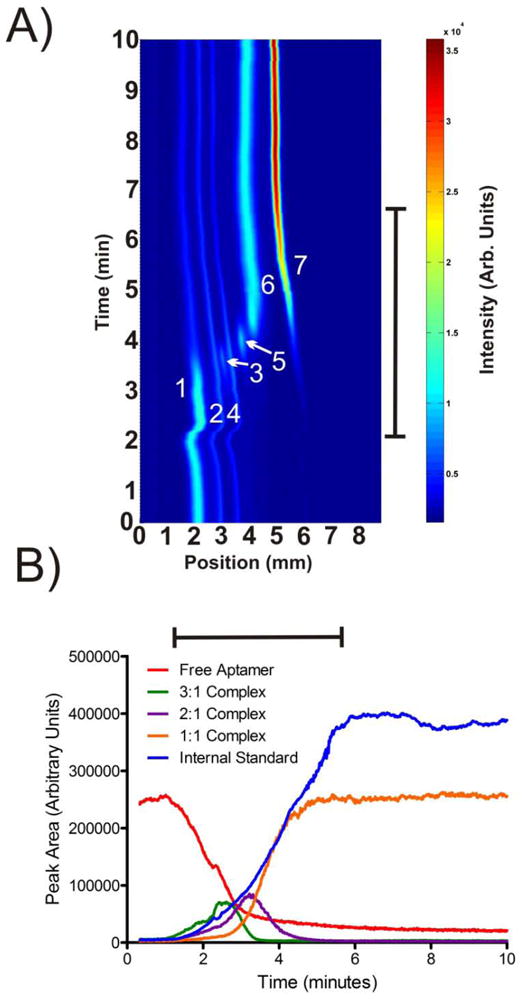
A) A contour plot showing subsequent μFFE linescans measured over time during the HIV-RT concentration gradient. Peaks are identified as 1) free aptamer, 2) aptamer impurity, 3) 3:1 aptamer: HIVRT complex, 4) aptamer impurity, 5) 2:1 aptamer: HIVRT complex, 6) 1:1 aptamer: HIVRT complex, and 7) internal standard (rhodamine 110). The anode is on the left. B) A plot of peak area over time for the free aptamer, 3:1, 2:1, 1:1 complexes and the internal standard. The black bars denote the 5 minute period over which HIV-RT concentration was increased from 0 to 500 nM.

Conclusions

We have demonstrated the use of gradient μFFE to measure equilibria between aptamers and their targets. The nearly continuous measurements allowed equilibria to be assessed at 300 discrete ligand concentrations in 5 minutes. This large data set allowed dissociation constants to be estimated with relatively narrow confidence intervals. Measurement of such a large number of ligand concentrations also made observation of complex stiochiometries possible. This technique could easily be applied to other equilibrium systems that generate a mobility shift upon binding including protein-protein interactions.

References

- 1.Hoffstetter-Kuhn S, Kuhn R, Wagner H. Electrophoresis. 1990;11:304–309. doi: 10.1002/elps.1150110406. [DOI] [PubMed] [Google Scholar]
- 2.Hoffstetter-Kuhn S, Wagner H. Electrophoresis. 1990;11:451–456. doi: 10.1002/elps.1150110603. [DOI] [PubMed] [Google Scholar]
- 3.Rodkey LS. Applied and Theoretical Electrophoresis. 1990;1:243–247. [PubMed] [Google Scholar]
- 4.Raymond D, Manz A, Widmer HM. Anal Chem. 1994;66:2858–2865. [Google Scholar]
- 5.Raymond D, Manz A, Widmer HM. Anal Chem. 1996;68:2515–2522. doi: 10.1021/ac950766v. [DOI] [PubMed] [Google Scholar]
- 6.Kobayashi H, Shimamura K, Akaida T, Sakano K, Tajima N, Funazaki J, Suzuki H, Shinohara E. J Chromatography A. 2003;990:169–178. doi: 10.1016/s0021-9673(02)01964-7. [DOI] [PubMed] [Google Scholar]
- 7.Fonslow BR, Bowser MT. Anal Chem. 2005;77:5706–5710. doi: 10.1021/ac050766n. [DOI] [PubMed] [Google Scholar]
- 8.Fonslow BR, Barocas V, Bowser MT. Anal Chem. 2006;78:5369–5374. doi: 10.1021/ac060290n. [DOI] [PubMed] [Google Scholar]
- 9.Janasek DS, Michael, Manz Andreas, Franzke Joachim. Lab on a Chip. 2006;6:710–713. doi: 10.1039/b602815b. [DOI] [PubMed] [Google Scholar]
- 10.Xu Y, Zhang CX, Janasek D, Manz A. Lab on a Chip. 2003;3:224–227. doi: 10.1039/b308476k. [DOI] [PubMed] [Google Scholar]
- 11.Janasek D, Schilling M, Franzke J, Manz A. Anal Chem. 2006;78:3815–3819. doi: 10.1021/ac060063l. [DOI] [PubMed] [Google Scholar]
- 12.Kohlheyer D, Besselink GAJ, Schlautmann S, Schasfoort RBM. Lab on a Chip. 2006;6:374–380. doi: 10.1039/b514731j. [DOI] [PubMed] [Google Scholar]
- 13.Zhang CX, Manz A. Anal Chem. 2003;75:5759–5766. doi: 10.1021/ac0345190. [DOI] [PubMed] [Google Scholar]
- 14.Kohlheyer D, Eijkel JCT, van den Berg A, Schasfoort RBM. Anal Chem. 2008;80:4111–4118. doi: 10.1021/ac800275c. [DOI] [PubMed] [Google Scholar]
- 15.Frost NW, Bowser MT. Lab Chip. 2009 doi: 10.1039/b922325h. in press. [DOI] [PMC free article] [PubMed] [Google Scholar]
- 16.Fonslow BR, Bowser MT. Anal Chem. 2006;78:8236–8244. doi: 10.1021/ac0609778. [DOI] [PubMed] [Google Scholar]
- 17.Kohlheyer D, Eijkel JCT, van den Berg A, Schasfoort RBM. Electrophoresis. 2008;29:977–993. doi: 10.1002/elps.200700725. [DOI] [PubMed] [Google Scholar]
- 18.Turgeon RT, Bowser MT. Analytical and Bioanalytical Chemistry. 2009;394:187–198. doi: 10.1007/s00216-009-2656-5. [DOI] [PMC free article] [PubMed] [Google Scholar]
- 19.Kostal V, Fonslow BR, Arriaga EA, Bowser MT. Anal Chem. 2009;81:9267–9273. doi: 10.1021/ac901508x. [DOI] [PMC free article] [PubMed] [Google Scholar]
- 20.Stone VN, Jaldock SJ, Croasdell LA, Dillon LA, Fielden PR, Goddard NJ, Thomas CLP, Brown BJT. J Chromatography A. 2007;1155:199–205. doi: 10.1016/j.chroma.2006.12.031. [DOI] [PubMed] [Google Scholar]
- 21.Turgeon RT, Bowser MT. Electrophoresis. 2009;30:1342–1348. doi: 10.1002/elps.200800497. [DOI] [PMC free article] [PubMed] [Google Scholar]
- 22.Fonslow BR, Bowser MT. Anal Chem. 2008;80:3182–3189. doi: 10.1021/ac702367m. [DOI] [PMC free article] [PubMed] [Google Scholar]
- 23.Chu YH, Avila LZ, Biebuyck HA, Whitesides GM. J Medicinal Chemistry. 1992;35:2915–2917. doi: 10.1021/jm00093a027. [DOI] [PubMed] [Google Scholar]
- 24.Chu YH, Lees WJ, Stassinopoulos A, Walsh CT. Biochemistry. 1994;33:10616–10621. doi: 10.1021/bi00201a007. [DOI] [PubMed] [Google Scholar]
- 25.Heegaard NHH, Robey FA. Anal Chem. 1992;64:2479–2482. doi: 10.1021/ac00045a004. [DOI] [PubMed] [Google Scholar]
- 26.Li C, Martin LM. Analytical and Bioanalytical Chemistry. 1998;263:72–78. doi: 10.1006/abio.1998.2791. [DOI] [PubMed] [Google Scholar]
- 27.Heegaard NHH. J Chromatography A. 1994;680:405–412. doi: 10.1016/0021-9673(94)85136-0. [DOI] [PubMed] [Google Scholar]
- 28.Rundlett K, Armstrong DW. Electrophoresis. 2001;22:1419–1427. doi: 10.1002/1522-2683(200105)22:7<1419::AID-ELPS1419>3.0.CO;2-V. [DOI] [PubMed] [Google Scholar]
- 29.Tao L, Kennedy RT. Electrophoresis. 1997;18:112–117. doi: 10.1002/elps.1150180121. [DOI] [PubMed] [Google Scholar]
- 30.Berezovski M, Krylov SN. J Am Chem Soc. 2002;124:13674–13675. doi: 10.1021/ja028212e. [DOI] [PubMed] [Google Scholar]
- 31.Berezovski M, Nutiu R, Li Y, Krylov SN. Anal Chem. 2003;75:1382–1386. doi: 10.1021/ac026214b. [DOI] [PubMed] [Google Scholar]
- 32.Wiegand TW, Williams PB, Dreskin SC, Jouvin MH, Kinet JP, Tasset D. J Immunology. 1996;157:221–230. [PubMed] [Google Scholar]
- 33.Mosing RK, Mendosa SD, Bowser MT. Anal Chem. 2005;77:6107–6112. doi: 10.1021/ac050836q. [DOI] [PubMed] [Google Scholar]
- 34.Shackman JG, Watson CJ, Kennedy RT. J Chromatogr A. 2004;1040:273–282. doi: 10.1016/j.chroma.2004.04.004. [DOI] [PubMed] [Google Scholar]
- 35.Shackman JG, Watson CJ, Kennedy RT. J Chromatogr A. 2004;1040:273–282. doi: 10.1016/j.chroma.2004.04.004. [DOI] [PubMed] [Google Scholar]
- 36.Tice JD, Song H, Lyon AD, Ismagilov RF. Langmuir. 2003;19:9127–9133. [Google Scholar]
- 37.Newman SA, Rossi G, Metzger H. Proceedings of the National Academy of Sciences of the United States of America. 1977;74:869–872. doi: 10.1073/pnas.74.3.869. [DOI] [PMC free article] [PubMed] [Google Scholar]
- 38.German I, Buchanan DD, Kennedy RT. Anal Chem. 1998;70:4540–4545. doi: 10.1021/ac980638h. [DOI] [PubMed] [Google Scholar]
- 39.Mendonsa SD, Bowser MT. Analytical Chemistry. 2004;76:5387–5392. doi: 10.1021/ac049857v. [DOI] [PubMed] [Google Scholar]
- 40.Mendonsa SD, Bowser MJ. Journal of the American Chemical Society. 2004;126:20–21. doi: 10.1021/ja037832s. [DOI] [PubMed] [Google Scholar]
- 41.Fu H, Guthrie JW, Le XC. Electrophoresis. 2006;27:433–441. doi: 10.1002/elps.200500460. [DOI] [PubMed] [Google Scholar]