Kinematic state estimation and motion planning for stochastic nonholonomic systems using the exponential map

SUMMARY

A nonholonomic system subjected to external noise from the environment, or internal noise in its own actuators, will evolve in a stochastic manner described by an ensemble of trajectories. This ensemble of trajectories is equivalent to the solution of a Fokker–Planck equation that typically evolves on a Lie group. If the most likely state of such a system is to be estimated, and plans for subsequent motions from the current state are to be made so as to move the system to a desired state with high probability, then modeling how the probability density of the system evolves is critical. Methods for solving Fokker-Planck equations that evolve on Lie groups then become important. Such equations can be solved using the operational properties of group Fourier transforms in which irreducible unitary representation (IUR) matrices play a critical role. Therefore, we develop a simple approach for the numerical approximation of all the IUR matrices for two of the groups of most interest in robotics: the rotation group in three-dimensional space, SO(3), and the Euclidean motion group of the plane, SE(2). This approach uses the exponential mapping from the Lie algebras of these groups, and takes advantage of the sparse nature of the Lie algebra representation matrices. Other techniques for density estimation on groups are also explored. The computed densities are applied in the context of probabilistic path planning for kinematic cart in the plane and flexible needle steering in three-dimensional space. In these examples the injection of artificial noise into the computational models (rather than noise in the actual physical systems) serves as a tool to search the configuration spaces and plan paths. Finally, we illustrate how density estimation problems arise in the characterization of physical noise in orientational sensors such as gyroscopes.

1. Introduction

In robotic systems, sensors make observations about the state of the system and actuators change the state by moving the robot in space. The “kinematic state” (or configuration) of a quasi-static robot often can be viewed as an element of a Lie group, G.^§ For a system whose state is specified in part by a stochastic input, the state cannot be known or controlled exactly. For such systems, the best that one can do is to estimate the state, and make plans to evolve the state so as to achieve some desired goal in a probabilistic sense. In contrast, in motion planning scenarios, the injection of “artificial noise” into the computational models can serve as a tool to search the configuration spaces and plan paths by following paths of high probability.

For these reasons, methods for probability density estimation can play an important role in applications. Systems that have states that evolve on Lie groups include gyroscopic sensors, cart-like mobile manipulators (including a library robot implemented in our research group), and flexible needles with bevel tips used in minimally invasive medical treatment planning. After establishing a general theoretical framework, we address each of these topics later in the paper.

Several orientation sensing modalities exist for mobile robots and satellites. These include star trackers,^38,32 gyroscopes,^29,45 magnetometers,^33,34 and omnidirectional vision systems.^4,5 Each of these can use the concepts of IURs for SO(3) in one form or another. A detailed literature review of this area is presented in ref. [6] (Chapters 14 and 15).

Another area of robotics in which methods of group theory can be applied is nonholonomic motion planning. The problem of motion planning for nonholonomic robots has received significant attention within the robotics community over the past two decades. For a summary of the state of the art, see refs. [67,74,79,80]. One approach is to do planning in high-dimensional configuration space. In contrast, we follow the approach of doing planning in workspace variables, which can have a greatly reduced dimension relative to that of configuration spaces. This approach has been taken in a number of prior papers from our research group shown in refs. [73,78]. In particular, the inverse kinematics of hyper-redundant and binary manipulators using “workspace densities” has been pursued in refs. [72,75,76]. This approach was adapted for nonholonomic planning in ref. [77] by sampling allowable moves. In contrast to sampling, a Fokker–Planck equation can be written that describes the evolution of probability density⁷⁰. In cases when the probability density is highly concentrated, this can be approximated as a Gaussian distribution, and covariances can be propagated.^68,69,71 These variations on the general theme of propagating probability densities in the workspace of the robot will be pursued later in the paper.

The remainder of this paper is structured as follows. Section 2 reviews the relationship between Fokker–Planck equations and stochastic differential equations that describe processes in IRⁿ and in Lie groups. Section 3 reviews and develops theory for Fourier-based estimation on Lie groups. Section 4 applies this methodology to the state estimation and motion planning of the kinematic cart. Section 5 applies the same methodology to steering a flexible needle in three-dimensional space. Section 6 applies this theory to the attitude estimation problem when using an inertial navigation systems and examines the problem of extracting system noise parameters from measured data, which is a capability that is important for handling all of these systems. Finally, Section 7 gives conclusions.

2. Fokker–Planck Equations

A stochastic differential equation (or SDE) in IR^p is of the form

$$d\mathbf{x}(t)=\mathbf{h}(\mathbf{x}(t),t)dt+H(\mathbf{x}(t),t)d\mathbf{W}(t)$$ (1)

where x ∈ IR^p and W ∈ IR^m. Here the deterministic dynamical system dx/dt = h(x, t) is perturbed at every value of time by noise, or random forcing described by W(t) where W(t) is a vector of uncorrelated Wiener processes, each with unit strength and H ∈ IR^p×m is a matrix that scales and couples these noises. SDEs used in modeling can either be of Ito or Stratanovich type.⁵⁴ In cases when H (x(t), t) is independent of x, this distinction is not important.

The Fokker–Planck equation is a partial differential equation that governs the time evolution of a probability density function ρ(x, t). When (1) is interpreted as an Ito SDE, the Fokker–Planck equation is written explicitly as

$$\frac{\partial \rho (\mathbf{x},t)}{\partial t}+\sum _{i=1}^p\frac{\partial }{\partial x_i}(h_i(\mathbf{x},t)\rho (\mathbf{x},t))-\frac{1}{2}\sum _{i,j=1}^p\frac{{\partial }^2}{\partial x_i\partial x_j}\left(\sum _{k=1}^m{H}_{ik}{H}_{kj}^T\rho (\mathbf{x},t)\right)=0.$$ (2)

We present the result without proof. The methodology was first employed by Fokker⁵³ and Planck.⁶¹ Many good books explain the methodology thoroughly.^54,59,62,64 Rather than repeating this classical derivation, we present a derivation for the Lie group case. In fact, this result is also known as shown in refs. [51,55,56,57,58,60,63,65] but with the possible exception of ref. [52], we have not seen a presentation that is easy for engineers to understand. Therefore, we attempt such a presentation here.

Let ρ(g, t) denote a time-parameterized probability density function on a unimodular Lie group^‡ (e.g., the rotation or motion groups). That is,

$$\rho (g,t)\ge 0\text{and}{\int }_G\rho (g,t)dg=1$$

for all values of t ∈ IR⁺, and

$$\rho (g,0)=\delta (g).$$

The Dirac delta function for a unimodular Lie group is well defined. This and other definitions and proofs can be found in ref. [6].

As usual, the partial derivative with respect to time is defined as

$$\frac{\partial \rho }{\partial t}=\underset{\mathrm{\Delta }t\to 0}{lim}\frac{1}{\mathrm{\Delta }t}[\rho (g,t+\mathrm{\Delta }t)-\rho (g,t)].$$

However, for a process that evolves on a Lie group, we should have

$$\begin{array}{l}\rho (g,t+\mathrm{\Delta }t)={\int }_G\rho (h,t)\rho (h^{-1}\circ g,\mathrm{\Delta }t)dh\\ ={\int }_G\rho (h,\mathrm{\Delta }t)\rho (h^{-1}\circ g,t)dh.\end{array}$$

As in the proof of the classical Fokker–Planck equation, one substitutes this convolution integral into the definition of partial derivative, and computes

$$C={\int }_G\frac{\partial \rho }{\partial t}f(g)dg$$

where f(g) is an arbitrary function. Then one changes coordinates, and expands f(g) in a Taylor series. One can define a Taylor series expansion on a Lie group in a way that is analogous to the classical case. If X_i is a basis element of the Lie algebra ℊ, then the “right” Lie derivative $X_i^r$ is defined by shifting from the right side of the argument of a function f(g) as

$$X_i^{r}f(g)=\frac{d}{dt}{(f(g\circ exp(t{X}_i)))\mid }_{t=0}.$$ (3)

If ε_i is a small real number, then the Taylor series corresponding to small perturbations on the right side of the argument of the function is:

$$f\left(g\circ exp\left(\sum _i{\epsilon }_i{X}_i\right)\right)=f(g)+\sum _i{\epsilon }_i{X}_i^{r}f(g)+\frac{1}{2}\sum _i\sum _j{\epsilon }_i{\epsilon }_j{X}_i^r{X}_j^{r}f(g)+\cdots .$$

A left Lie derivative can be similarly defined, and

$$f\left(exp\left(\sum _i{\epsilon }_i{X}_i\right)\circ g\right)=f(g)+\sum _i{\epsilon }_i{X}_i^{l}f(g)+\frac{1}{2}\sum _i\sum _j{\epsilon }_i{\epsilon }_j{X}_i^l{X}_j^{l}f(g)+\cdots .$$

The differential operators $X_i^r$ and $X_i^l$ obey the product rule. Note that derivatives resulting from right shifts are left invariant, and those resulting from left shifts are right invariant.

When the stochastic process on the group defined by

$$g^{-1}dg=\mathit{\epsilon }\text{or}dg{g}^{-1}=\mathit{\epsilon }$$ (4)

is substituted into the Taylor series expansion to second order, where

$$\mathit{\epsilon }=\mathbf{h}(g,t)dt+H(g,t)d\mathbf{W}(t),$$

averages are then taken over the ensemble of all possible motions, and the properties of uncorrelated white noises are used to eliminate terms. Integration by parts then results in the localization of the form

$${\int }_{G}Ef(g)dg=0\to E=0$$

where E = 0 is the Fokker–Planck equation

$$\frac{\partial \rho (g,t)}{\partial t}+\sum _{i=1}^d{X}_i^{r,l}(h_i(g,t)\rho (g,t))-\frac{1}{2}\sum _{i,j=1}^d{X}_i^{r,l}{X}_j^{r,l}\left(\sum _{k=1}^m{H}_{ik}(g,t)H_{kj}^T(g,t)\rho (g,t)\right)=0.$$ (5)

The superscripts (r, l) are chosen depending on whether the SDE on the left or right of (4) is used, and d is the dimension of the Lie group. Examples of (5) will be demonstrated in subsequent sections in the context of gyroscopes, kinematic carts, and flexible needle steering. Focusing on the “r” case, when h and H are constant, we can write

$$\frac{\partial \rho (g,t)}{\partial t}+\sum _{i=1}^d{h}_i{X}_i^r\rho (g,t)-\frac{1}{2}\sum _{i,j=1}^d{D}_{ij}{X}_i^r{X}_j^r\rho (g,t)=0$$ (6)

where

$$D_{ij}=\sum _{k=1}^m{H}_{ik}{H}_{kj}^T.$$

When considering stochastic differential equations and the corresponding Fokker–Planck equations, it is usually important to specify whether the Ito or Stratanovich form is used. Without getting into too much detail, it suffices to say that the Ito form has been assumed in the derivation of both of the above Fokker–Planck equations. However, if the coloring matrices, H, are independent of the coordinates used (or do not depend explicitly on the group elements), then the Ito and Stratanovich forms of the Fokker–Planck equation will be identical. In the examples that we will consider, the Ito and Stratanovich forms of the Fokker–Planck equation are all the same unless otherwise specified.

3. Fourier-Based Estimation on Lie Groups and Applications

In estimation, one desires to obtain the underlying probability density function that describes the process giving rise to these data. There are two closely related variations of this problem. In the first, a set of randomly drawn group elements g₁, g₂, …, g_m are obtained and we seek to estimate the underlying density ρ(g). In the second variation, we sample the probability density itself at points on a grid, {g_i}, and we seek to evaluate (or interpolate) ρ(g) at any other value of g ∈ G. In this paper we develop techniques that allow both of these variations of the problem to be solved when G = SO(3). One kind of estimator in IRⁿ is the Fourier estimator.^23,25 This concept generalizes to Lie groups.^22,24 Abstract estimation problems on SO(3) and compact Lie groups in general have been reported elsewhere.^36,37

Both of the variations of the problem described above can be formulated as follows:

$${\rho }_{\mathit{samp}}(g)=\sum _{i=1}^m{\alpha }_i\delta (g_i^{-1}\circ g)$$

where δ(·) is the Dirac delta function for the group G and

$$\sum _{i=1}^m{\alpha }_i=1.$$

In the first variation of the problem, α_i = 1/m. In the second variation α_i = ρ(g_i). In order to define the appropriate concept of a Fourier estimator in this context, some review is required.

3.1. Group representations and harmonic analysis

A group representation can be thought of as a matrix-valued function of group-valued argument, U(g), with the homomorphism property:

$$U(g_1\circ g_2)=U(g_1)U(g_2).$$

Irreducibility means that it is not possible to simultaneously block-diagonalize U(g) by the same similarity transformation for all values of g in the group. Completeness of a set of representations means that every (reducible) representation can be decomposed into a direct sum of the representations in the set. A famous result (due to Schur) states that every irreducible representation is equivalent to a unitary one. Therefore, without loss of generality we can take U to be unitary, i.e., U⁻¹ = U^* where * denotes the Hermitian conjugate. It then follows that since,

$$I=U(e)=U(g^{-1}\circ g)=U(g^{-1})U(g),$$

then

$$U(g^{-1})={(U(g))}^{-1}=U^{\ast }(g).$$

In a number of practical applications, data is presented on Lie groups such as the rotation group and group of rigid-body motions. These are noncommutative groups for which the representation theory and harmonic analysis have been fully worked out (see e.g., refs. [7,8,16,17,21]). In particular, the method of induced representations⁹ was used by Miller for the case of the rigid-body motion group.¹³ Connections between group representations and special functions are explored in refs. [12, 19]. Representations of the rotation group play a central role in quantum mechanics.^7,18,20 In that application, the Euler angles are used to parameterize rotations. This corresponds to the double-coset decomposition used in refs. [10,11] for FFTs developed for the rotation group, SO(3).

In their most general form, the results of this paper are as follows, where G is a unimodular Lie group (e.g., SO(3), SE(2), SE(3)). Given functions f_i (g) for i = 1, 2 which are square integrable with respect to a bi-invariant integration measure dg on a the group (G, ◦), we can define the convolution product

$$(f_1\ast f_2)(g)={\int }_G{f}_1(h)f_2(h^{-1}\circ g)dh,$$

and the Fourier transform

$$\mathcal{F}(f)(\lambda )={\int }_{G}f(g)U(g^{-1},\lambda )dg$$

where U(·, λ) is a unitary matrix function (called an irreducible matrix representation) for each value of the parameter λ (where the set of all values of λ is called the dual of the group, and is denoted as Ĝ).

The shorthand ℱ(f)(λ) = f̂(λ) is often convenient. The Fourier transform defined in this way has corresponding inversion, convolution, and Parseval theorems:

$$\begin{array}{c}f(g)=\sum _{\lambda \in \widehat{G}}d(\lambda )\text{trace}[\widehat{f}(\lambda )U(g,\lambda )],\\ \mathcal{F}(f_1\ast f_2)(\lambda )={\widehat{f}}_2(\lambda ){\widehat{f}}_1(\lambda )\end{array}$$ (7)

and

$${\int }_G\mid f(g){\mid }^{2}dg=\sum _{\lambda \in \widehat{G}}d(\lambda ){\left|\right|\widehat{f}(\lambda )\left|\right|}^2.$$

Here ||·|| is the Hilbert–Schmidt (Frobenius) norm, and d(λ) is the dimension of the matrix U(g, λ). Much of this is classical mathematics (see e.g., ref. [15]), which has not been fully embraced by the engineering world until relatively recently.⁶

A useful definition is

$$u(X_i,\lambda )={U(exp(t{X}_i),\lambda )\mid }_{t=0}.$$

We develop explicit expressions for U(g, λ) and u(X_i, λ) using the exponential map and corresponding parameterizations for the groups SO(3), SE(2) and SE(3). In particular, given the scalar parameters x_i ∈ IR, the linearity of the Lie algebra allows one to write

$$u\left(\sum _i{x}_i{X}_i,\lambda \right)=\sum _i{x}_{i}u(X_i,\lambda )$$

and a famous theorem states that^7,14,6:

$$U\left(exp\left(\sum _i{x}_i{X}_i\right),\lambda \right)=expu\left(\sum _i{x}_i{X}_i,\lambda \right).$$ (8)

These results together with the surjectivity of the exponential map (up to a set of measure zero) and the sparseness of the matrices u(X_i, λ) provides the properties that we exploit for the rapid evaluation of U(g, λ).

This all relates back to the problem of density estimation on G as follows. The Fourier matrices corresponding to ρ_samp(g) are computed as

$$\begin{array}{l}\mathcal{F}({\rho }_{\mathit{samp}})(\lambda )=\sum _{i=1}^m{\alpha }_i{\int }_G\delta \left(g_i^{-1}\circ g\right)U(g^{-1},\lambda )dg\\ =\sum _{i=1}^m{\alpha }_{i}U(g_i^{-1},\lambda )=\sum _{i=1}^m{\alpha }_i{U}^{\ast }(g_i,\lambda ).\end{array}$$

Substitution into the Fourier inversion formula,

$${\rho }_{\mathit{est}}(g)=\sum _{\lambda \in \widehat{\widehat{G}}}\text{trace}({\widehat{\rho }}_{\text{samp}}(\lambda )U(g,\lambda ))d(\lambda ).$$

or

$${\rho }_{\mathit{est}}(g)=\sum _{i=1}^m{\alpha }_i\sum _{\lambda \in {\widehat{G}}_T}\text{trace}\left(U\left(g_i^{-1}\circ g,\lambda \right)\right)d(\lambda ).$$ (9)

Here Ĝ_T denotes the truncated/bandlimited version of the dual space Ĝ. Since Ĝ_T ≠ Ĝ, it follows that ρ_est(g) ≠ ρ_samp(g). The function ρ_est (g) is a smoothed version of ρ_samp(g) that can be evaluated at group elements g ≠ g_i.

3.1.1. Example 1: the SO(3) case

In the particular case of SO(3), the basis elements for the Lie algebra so(3) are

$$X_1=\left(\begin{array}{ccc}0& 0& 0\\ 0& 0& -1\\ 0& 1& 0\end{array}\right);X_2=\left(\begin{array}{lll}0\hfill & 0\hfill & 1\hfill \\ 0\hfill & 0\hfill & 0\hfill \\ -1\hfill & 0\hfill & 0\hfill \end{array}\right);X_3=\left(\begin{array}{ccc}0& -1& 0\\ 1& 0& 0\\ 0& 0& 0\end{array}\right).$$

Exponentiating any linear combination of these basis elements yields an element of the rotation group, SO(3), as reviewed in refs. [6,48–50]. In this case, the set of IUR matrices is indexed by λ = l where l = 0, 1, 2, 3, ··· and each IUR is a (2l + 1) × (2l + l) matrix. The m, nth entry of the l^th matrix is of the form⁶:

$$\begin{array}{l}{u}_{mn}^l(X_1)=\frac{i}{2}(c_{-n}^l{\delta }_{m+1,n}+c_n^l{\delta }_{m-1,n})\\ u_{mn}^l(X_2)=\frac{1}{2}(-c_{-n}^l{\delta }_{m+1,n}+c_n^l{\delta }_{m-1,n})\\ u_{mn}^l(X_3)={-in\delta }_{m,n}\end{array}$$

where −l ≤ m, n ≤ l and $c_n^l=\sqrt{(l-n)(l+n+1)}$.

If we define

$$u^l(x_1,x_2,x_3)=\sum _{k=1}^3{x}_k{u}^l(X_k)$$

where $X={\sum }_{k=1}^3{x}_k{X}_k$, then as stated earlier, the exponential of this (2l + 1) × (2l + 1) matrix will be an irreducible unitary representation of SO(3) expressed in terms of the exponential coordinates for SO(3).

3.1.2. Example 2: the SE(2) case

The SE(2)-Fourier transform, as expressed in the coordinates x, y, θ, or equivalently in the polar coordinates (r cos φ, r sin φ, θ), has been used previously to solve similar equations in a variety of different applications.^71,72 We note here an alternative approach. Even though the IURs of SE(2) are infinite dimensional, it is possible to approximate them as finite unitary matrices by using (8) in truncated form. In particular, for SE(2) a set of basis elements for the Lie algebra are:

$$X_1=\left(\begin{array}{ccc}0& 0& 1\\ 0& 0& 0\\ 0& 0& 0\end{array}\right);X_2=\left(\begin{array}{ccc}0& 0& 0\\ 0& 0& 1\\ 0& 0& 0\end{array}\right);X_3=\left(\begin{array}{ccc}0& -1& 0\\ 1& 0& 0\\ 0& 0& 0\end{array}\right).$$

The corresponding Lie algebra representation matrices are:

$$u_{mn}(X_1,p)=\frac{ip}{2}({\delta }_{m,n+1}+{\delta }_{m,n-1})$$ (10)

$$u_{mn}(X_2,p)=\frac{p}{2}({\delta }_{m,n+1}-{\delta }_{m,n-1})$$ (11)

$$u_{mn}(X_3,p)=-{im\delta }_{m,n}$$ (12)

where in the SE(2) case λ = p takes continuous values over all of the nonnegative real numbers, and in the Fourier inversion formula the sum over λ is replaced by an integral over p with measure pdp/4π². These u_mn(X_k, p) are infinite-dimensional sparse skew-Hermitian matrices, which when truncated to a finite range −d ≤ m, n ≤ d results in (2d + 1) × (2d + 1) matrices. The truncation does not change their skew-Hermitian nature, and exponentiation of these matrices results in unitary matrices that approximate the IURs for SE(2). This approximation becomes better as d becomes large.

3.2. Solving Fokker–Planck equations using harmonic analysis

By the definition of the group Fourier transform ℱ[·] and operators $X_i^r$ reviewed earlier in this paper, one observes that

$$\mathcal{F}[X_i^{r}f]={\int }_G\frac{d}{dt}{(f(g\circ exp(t{X}_i)))\mid }_{t=0}U(g^{-1},\lambda )dg.$$ (13)

By performing the change of variables h = g ◦ exp(tX_i) and using the homomorphism property of the representations U(·,λ), one finds

$$\mathcal{F}[X_i^{r}f]={\int }_{G}f(h)\frac{d}{dt}{(U(exp(t{X}_i)\circ h^{-1},\lambda ))\mid }_{t=0}dh$$ (14)

$$=\frac{d}{dt}{(U(exp(t{X}_i),\lambda ))\mid }_{t=0}{\int }_{G}f(h)U(h^{-1},\lambda )dh.$$ (15)

By defining

$$u(X_i,\lambda )=\frac{d}{dt}{(U(exp(t{X}_i),\lambda ))\mid }_{t=0},$$

we write

$$\mathcal{F}[X_i^{r}f]=u(X_i,\lambda )\widehat{f}(\lambda ).$$

Hence, (6) can be transformed to the system of linear differential equations:

$$\frac{d\widehat{\rho }}{dt}=\mathcal{B}(\lambda )\widehat{\rho },$$ (16)

subject to the identity matrix as initial conditions, where

$$\mathcal{B}(\lambda )=\frac{1}{2}\sum _{k,l=1}^n{D}_{lk}u(X_l,\lambda )u(X_k,\lambda )-\sum _{l=1}^n{h}_{l}u(X_l,\lambda ).$$

In principle, ρ(g; t) is then found by simply substituting ρ̂(λ; L) = exp(Lℬ(λ)) into the the group Fourier inversion formula (7).

3.3. Shifted Gaussian solution for Fokker–Planck equations with small diffusion

In this subsection, we show that the solution for the Fokker–Planck equations can be approximated by the shifted Gaussian when the diffusion is small. Even though we describe the SE(3) case here, similar arguments are possible for the SE(2) case.

A driftless diffusion equation on SE(3) is of the form:

$$\left(\frac{\partial }{\partial t}-\frac{1}{2}\sum _{k,l=1}^6{D}_{lk}{X}_l^R{X}_k^R\right)f=0,$$ (17)

which subject to the initial conditions f(g, 0) = δ(g). For intermediate to large values of t such equations can be solved efficiently using methods from harmonic analysis as seen in earlier section. However, for small values of t, such methods become impractical due to Gibbs peaks and the large number of harmonics required. In contrast, as will be seen in Section 6.2.1., the concentrated Gaussian distributions provide a closed-form solution in the small t limit. A highly concentrated Gaussian distribution on SE(3) can be defined as shown in ref. [71]

$$\rho (g;\mathrm{\sum })=c(\mathrm{\sum })exp\left(-\frac{1}{2}{\mathbf{x}}^T{\mathrm{\sum }}^{-1}\mathbf{x}\right),$$ (18)

where $g=exp(\widehat{\mathbf{x}})=exp\left({\sum }_{i=1}^6{x}_i{X}_i\right)$ with {X_i} denoting the standard basis for the Lie algebra se(3), and c(Σ) = (2π)^−3/2| det(Σ)|^−1/2. A small-time solution to (17) is f(g, t) = ρ(g; tD).

If the drift term is added to (17), thus resulting in an equation of the form (6), the solution of this modified system can be approximated by the shifted Gaussian in the very small noise limit. Namely, this approximated solution has the form of (18) and $\mathbf{x}=log{(g_m^{-1}(t)\circ g)}^{\vee }$, where g_m(t) is the mean path. In this case, the covariance matrix can be computed by covariance propagation. The covariance propagation in ref. [71] is based on the concatenation of a finite number of noisy motions. In the limiting case of a time-parameterized path of noisy motions, the covariance propagation formula can be written as

$${\mathrm{\sum }}_t={\int }_0^t{Ad}_{g_m^{-1}(\tau )g_m(t)}^{-1}D{Ad}_{g_m^{-1}(\tau )g_m(t)}^{-T}d\tau$$ (19)

where Ad_g(·) is the adjoint. Technically, the mean path, g_m(t) is not the same as the noiseless path that can be obtained by solving the deterministic model. Referring back to the drift coefficients {h_i} in (6), the path that the solution would follow if all D_ij = 0 would be $exp({\sum }_{i=1}^6{h}_i{X}_i)$. While this is not exactly equal to g_m(t), in practice we use the noiseless path for the mean path since it is easier to have the noiseless path than the mean path and the difference between the two can be assumed to be small in the case of small diffusion. This approach will be used for path planning for the cart and the flexible needle in subsequent sections.

4. Estimation and Motion Planning for the Stochastic Kinematic Cart

In this section, a stochastic version of the kinematic cart is considered. We first address the problem of estimating the position and orientation of the cart when nothing but a history of noisy wheel angles is given (i.e., dead reckoning). Then we address how to use the probabilistic information obtained by solving Fokker–Planck equations for the purpose of planning.

4.1. Pose estimation for the stochastic cart

Consider the kinematic cart shown in Fig. 1(a). The position of the cart is (x, y) and the orientation is θ. Here L is the length of the wheel base (distance between the wheels as measured along the axis), r is the radius of the wheels, φ₁ is the angle through which the right wheel rotates, and φ₂ is the angle through which the left wheel rotates. Both of these angles are measured counterclockwise when viewed along the axel from outside the cart to the left side. This is perhaps the most common geometry for mobile robots used in robotics research. For example, the mobile manipulator shown in Fig. 1(b) was developed by our research group for the purpose of retrieving books from library shelves and moves as a kinematic cart.

Fig. 1.

The kinematic cart: (a) definition of variables; (b) the CAPM library robot from our lab as an example of a mobile manipulator with cart as the base.

The infinitesimal motions of the kinematic cart are governed by no-lateral-slip conditions, which allow the following transverse translational motions and rotations:

$$\left(\begin{array}{c}dx\\ dy\\ d\theta \end{array}\right)=\left(\begin{array}{cc}\frac{r}{2}cos\theta & \frac{r}{2}cos\theta \\ \frac{r}{2}sin\theta & \frac{r}{2}sin\theta \\ \frac{r}{L}& -\frac{r}{L}\end{array}\right)\left(\begin{array}{c}{d\phi }_1\\ {d\phi }_2\end{array}\right).$$

If the infinitesimal changes in wheel rotation angles are of the form

$${d\phi }_i={\omega }_{i}dt+\sigma {dW}_i$$

where dW_i are increments of unit-strength Wiener processes, σ allows us to specify the strength, and the commanded wheel angle rates are ω₁ = ω + Δ and ω₂ = ω − Δ, then the result is the stochastic differential equation:

$$\left(\begin{array}{c}dx\\ dy\\ d\theta \end{array}\right)=\left(\begin{array}{c}r\omega cos\theta \\ r\omega sin\theta \\ \alpha \end{array}\right)dt+\sigma \left(\begin{array}{cc}\frac{r}{2}cos\theta & \frac{r}{2}cos\theta \\ \frac{r}{2}sin\theta & \frac{r}{2}sin\theta \\ \frac{r}{L}& -\frac{r}{L}\end{array}\right)\left(\begin{array}{c}{dW}_1\\ {dW}_2\end{array}\right).$$ (20)

where α = 2rΔ/L.

If the specified speeds of the wheels are either constant, or explicit functions of time (without dependence on time through x(t) = [x(t), y(t), θ(t)]^T), then by using the Fokker–Planck Eq. (2) results in:

$$\frac{\partial f}{\partial t}=-r\omega cos\theta \frac{\partial f}{\partial x}-r\omega sin\theta \frac{\partial f}{\partial y}-\alpha \frac{\partial f}{\partial \theta }+\frac{1}{2}{\sigma }^2\left[\frac{r^2}{2}{cos}^2\theta \frac{{\partial }^{2}f}{{\partial x}^2}+r^{2}sin\theta cos\theta \frac{{\partial }^{2}f}{\partial x\partial y}+\frac{r^2}{2}{sin}^2\theta \frac{{\partial }^{2}f}{{\partial y}^2}+\frac{2r^2}{L^2}\frac{{\partial f}^2}{{\partial \theta }^2}\right].$$ (21)

Of course, this system is evolving on the group of rigid-body motions of the plane, SE(2), which has group elements that can be described in the form

$$g=\left(\begin{array}{ccc}cos\theta & -sin\theta & x\\ sin\theta & cos\theta & y\\ 0& 0& 1\end{array}\right).$$

The reason why we can use (2) is that the bi-invariant integration measure for SE(2) is dg = dxdydθ, and so, to within a set of measure zero, SE(2) “looks like” the slab within IR³ defined by θ ∈ (−π, π) to a sufficient degree that we can use the Fokker–Planck machinery developed for Euclidean space.

On the other hand, we can view the same problem from a coordinate-free point of view. Recall that for SE(2), the ∨ operation is defined as

$${\left(\begin{array}{ccc}0& -\omega & v_1\\ \omega & 0& v_2\\ 0& 0& 0\end{array}\right)}^{\vee }=\left(\begin{array}{c}{v}_1\\ v_2\\ \omega \end{array}\right).$$

Realizing that

$${(g^{-1}\stackrel{.}{g})}^{\vee }=J(\mathbf{x})\stackrel{.}{\mathbf{x}}$$

where

$$\begin{array}{l}J(\mathbf{x})=\left[{\left(g^{-1}\frac{\partial g}{\partial x}\right)}^{\vee },{\left(g^{-1}\frac{\partial g}{\partial y}\right)}^{\vee },{\left(g^{-1}\frac{\partial g}{\partial \theta }\right)}^{\vee }\right]\\ =\left(\begin{array}{ccc}cos\theta & sin\theta & 0\\ -sin\theta & cos\theta & 0\\ 0& 0& 1\end{array}\right)\end{array}$$

allows us to write (20) (viewed as a Stratanovich SDE) in the coordinate-free form:

$${(g^{-1}dg)}^{\vee }=\left(\begin{array}{c}r\omega \\ 0\\ \alpha \end{array}\right)dt+\sigma \left(\begin{array}{cc}\frac{r}{2}& \frac{r}{2}\\ 0& 0\\ \frac{r}{L}& -\frac{r}{L}\end{array}\right)\left(\begin{array}{c}{dW}_1\\ {dW}_2\end{array}\right).$$ (22)

This result is obtained by simply multiplying both sides of (20) by J(x). Note that the h and H in (22) are independent of g. When the SDE is written in the form of (22) the no-slip condition that results in the nonholonomic behavior of the system is clear from the zeros in the middle row.

Equating (g⁻¹dg)^∨ with ε and using (5) for this system, the resulting invariant form of this SDE is:

$$\frac{\partial f}{\partial t}=-r\omega X_1^{r}f-\alpha X_3^{r}f+\frac{1}{2}{\sigma }^2\left[\frac{r^2}{2}{(X_1^r)}^2+\frac{{2r}^2}{L^2}{(X_3^r)}^2\right]f.$$

4.2. Stochastic motion planning for the cart

In this subsection, several related approaches to motion planning of the kinematic cart are demonstrated for both the case when the workspace is free of obstacles and the case when obstacles are present. Three variations of the Fokker–Planck/SDE approach are taken: (1) The Fokker–Planck equation is solved explicitly using the approximate IURs and Fourier diffusion matrix resulting from truncating and exponentiated the sparse infinite-dimensional se(2) Lie algebra representation matrices; (2) in cases where the magnitude of the noise is assumed to be small, covariances are propagated and probability densities are evaluated by shifting closed-form Gaussian distributions along the drift path; (3) sample paths of the SDE are generated and histograms are formed. Hybrid approaches that combine these techniques can also be taken. Methods (1) and (2) work well in the case when there are no obstacles. However, they must be augmented to take into account obstacles. This is easy to do with method (3) where sample paths are removed from the ensemble if any point on a path intersects an obstacle. These methods are described in detail in the following two subsections.

4.2.1. The cart in an environment without obstacles

Consider the following scenario: Suppose that we want to generate a path for the kinematic cart from (x, y, θ) = (0, 0, 0) to (2, 0.5, π/4). How can we do this? One approach could be to use sinusoids⁶⁷ or some other weighted sum of basis (or modal) functions as the input for the wheel angles. Then the unknown coefficients { $a_j^i$} in the expression ${\phi }_i(t)={\sum }_{j=1}^N{a}_j^i{\mathrm{\Phi }}^j(t)$ for the wheel angles φ₁ and φ₂ can be found by numerically integrating the nonholonomic kinematic equations and using iterative numerical procedures similar to those used in the inverse kinematics of hyper-redundant manipulators (see ref. [81] for details). If the system were completely deterministic (no actuator noise, and no slipping of the wheels), this approach might work well. However, in the stochastic case, an ensemble of paths will result, and the probability of actually reaching a specific neighborhood of the goal will depend on the amount of noise in the system. Therefore, we propose to use here the path-of-probability (or POP) algorithm proposed in refs. [75,76]. In this algorithm, each move is taken so as to maximize the probability density that remains to reach the goal. And one of the nice features of this algorithm is that we do not even have to know a priori a path that deterministically connects the initial and final states of the system. For example, if we want to steer the cart so as to go from (x, y, θ) = (0, 0, 0) to (2, 0.5, π/4), we can use as the deterministic drift which corresponds to both wheels moving forward with speed 1. Then, in the deterministic case, the resulting pose at time t would be (rt, 0, 0). Even though this is not the desired pose, if the Fokker–Planck equation resulting from this drift term and some noise causes there to be nonzero probability density over the desired pose, then the POP algorithm can be used to find a path. The intermediate step, g_i can be determined by

$$g_i=\underset{g\in S}{argmax}\rho (g^{-1}\circ g_{\mathit{goal}};\tau ),$$

where τ is the remaining time to hit the goal and S is the set of possible intermediate paths generated by numerical integration of SDE. We use Euler–Maruyama numerical integration method.⁶⁶

The path planning results using the first method described in Section 4.2 are shown in Fig. 2. Using approximate IURs and Fourier diffusion matrix, we can obtain the solution to the Fokker–Planck equation, which is the probability density function. This PDF is used for the POP algorithm. The cart starts from (x, y, θ) = (0, 0, 0) and the triangle in the figures shows the position and orientation of the goal. The noise constant, σ = 0.3 was used in (22).

Fig. 2.

Path planning for the kinematic cart using IURs and harmonic analysis: (a) Cart path for the goal, (x, y, θ) = (2, 0.5, π/4) (b) Cart path for the goal, (x, y, θ) = (1.6, 1.6, π/3).

The path planning results by the shifted Gaussian are shown in Fig. 3. Unlike the harmonic analysis method, the shifted Gaussian method can be applied to the small diffusion case. The dash lines in Fig. 3 are the noiseless paths. Note that the goal is not far from the noiseless path. The constant, α = 0.11 was used for the noiseless path in Fig. 3(b). For both cases, the noise constant, σ = 0.02 was used.

Fig. 3.

Path planning for the kinematic cart using the shifted Gaussian: (a) Cart path for the goal, (x, y, θ) = (2.5, 0.2, 0); (b) Cart path for the goal, (x, y, θ) = (2.0, 1.4, π/3).

4.2.2. The cart in an environment with obstacles

When obstacles are present in the environment, the Fokker–Planck approach and covariance propagation break down since they do not take into account obstacles. There are several modifications that can be attempted in special cases. For example, one can ignore the obstacles, and use this approach, and if the resulting path does not hit an obstacle, then it will have produced a valid result. Closely related to this would be to propagate probability densities forward from the initial state until the amount of probability density situated over the obstacles reaches some threshold value, and then stop. Then do the same by propagating probability density backward from the goal. If there exists an overlapping region in the workspace (which is a bounded subset of SE(2)) where the product of these probability densities is nonzero, then the POP algorithm can be used to generate paths to and from via points within these regions. The resulting composite paths will be guaranteed not to intersect obstacles. Alternatively, the obstacles can be represented using artificial potentials that can be incorporated into the Fokker–Planck equations. Unfortunately, the resulting equations are difficult to solve.

While the techniques outlined above may work in specialized cases, it is desirable to have algorithms that work in general. We simply generate many sample paths by integrating the SDE describing the stochastic cart. This integration can be implemented by the Euler–Maruyama method⁶⁶. Each time we check for overlaps of the positional part of the poses that constitute each path against the positions on the surface of the obstacles. If at any time step a path penetrates the surface of an obstacle, we kill this path and then initiate a new sample path. After a large number of obstacle-avoiding sample paths are generated, a PDF of the reachable positions and orientations is generated. However, a big difference between the case with obstacles and the case without obstacles is that the PDF is now dependent on the starting point. This means that after each move of the robot, a new ensemble of sample paths must be generated. In other words, we cannot simply generate PDFs and shift them as we move as is done in the obstacle-free version of POP. Rather, we must recompute PDFs after each move. The reason for this is that the relative location of obstacles (and their influence on the evolution of probability density) changes with respect to the cart as it moves.

In order to have a smooth PDF from a finite number of path samples, we assigned a small Gaussian function to each path sample and averaged an ensemble of the Gaussian functions. The path planning results by this approach are shown in Fig. 4 and Fig. 5. Alternatively, we can estimate the PDF by a Gaussian function from the sample paths. The mean and the covariance of the Gaussian can be estimated from the sample paths. Using this approach, we have the results as shown in Fig. 6.

Fig. 4.

Path planning for the kinematic cart using many sample paths: (a) Cart path for the goal, (x, y, θ) = (1.6, 1.6, π/3) (b) Cart path for the goal, (x, y, θ) = (1.6, 1.6, π/3), the obstacle position = (0.75, 0.75) and the obstacle radius = 0.25.

Fig. 5.

Path planning for the kinematic cart using many sample path: (a) Cart path for the goal, (x, y, θ) = (2, 0.5, π/4) (b) Cart path for the goal, (x, y, θ) = (2, 0.5, π/4), the obstacle position = (1, 0) and the obstacle radius = 0.25.

Fig. 6.

Path planning for the kinematic cart by many sample paths. The mean and the covariance from the paths are used for a Gaussian function: (a) Cart path for the goal, (x, y, θ) = (1.6, 1.6, π/3) (b) Cart path for the goal, (x, y, θ) = (1.6, 1.6, π/3), the obstacle position = (0.5, 0.5) and the obstacle radius = 0.25.

5. Stochastic Motion Planning for the Flexible Needle with Bevel Tip

Recently, a number of works have been concerned with the steering of flexible needles with bevel tips through soft tissue for minimally invasive medical treatments.^82,83,84 In this scenario, a flexible long needle with a bevel tip bends as it is inserted into the tissue. The question becomes how to specify a time-history of the control variables (pushes and twists of the needle at the insertion point) to deliver the needle tip to the desired location within the tissue. In this section, we apply the shifted Gaussian to have the probability density function of the flexible needle, and solve the path planning problem using the PDF.

Figure 7 depicts the needle and the body fixed frame. The needle is rotated with the angular velocity, ω, while it is inserted with the insertion velocity, v. It follows an arc whose curvature is κ. Using this body fixed frame, the nonholonomic kinematic model for the needle was developed in ref. [82] as:

$$\xi ={(g^{-1}\stackrel{.}{g})}^{\vee }={[\kappa 0\omega 00v]}^T$$ (23)

Fig. 7.

The definition of parameters and frames in the nonholonomic needle model.⁸³

In order to get a noise model for the needle, we assume that

$$\omega (t)={\lambda }_1{w}_1(t),$$

and

$$v(t)=1+{\lambda }_2{w}_2(t)$$

in the similar way in ref. [83]. w_i (t) is the unit Gaussian white noise. Thus, our noise model is

$$\xi ={(g^{-1}\stackrel{.}{g})}^{\vee }dt=\left[\begin{array}{c}\kappa \\ 0\\ 0\\ 0\\ 0\\ 1\end{array}\right]dt+\left[\begin{array}{cc}0& 0\\ 0& 0\\ {\lambda }_1& 0\\ 0& 0\\ 0& 0\\ 0& {\lambda }_2\end{array}\right]\left[\begin{array}{c}{dW}_1\\ {dW}_1\end{array}\right]$$ (24)

where dW = W (t + dt) − W (t) = w(t)dt are the non-differentiable increments of a Wiener process W (t). This noise model can be seen as a stochastic differential equation. If the noise is small, which means the small diffusion, the solution to the corresponding Fokker–Planck equation can be approximated by the shifted Gaussian function as explained in Section 3.3.

For a numerical example, the values of λ₁ and λ₂ are both set to be 0.08. Figure 8 shows the path planing results using the concentrated shifted Gaussian distribution. The number of intermediate steps used in the path generation is 10. In this example, only positions of the goal is considered in path planning since the specific needle orientation is less important than the position in the needle insertion system. This can be achieved by the marginal density function. Our full density function from shifted Gaussian approach is a six-dimensional function, and the three-dimensional marginal density function can be obtained by integrating it over orientational space.

Fig. 8.

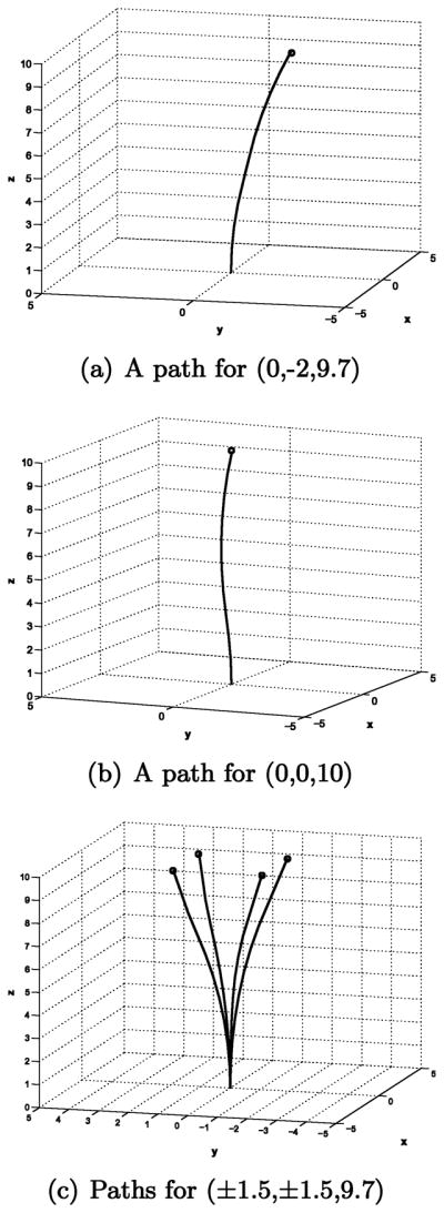
Path generation using concentrated shifted Gaussian distribution: κ = 0.05, λ₁ = 0.08, and λ₂ = 0.08.

6. Attitude Estimation Using an Inertial Navigation System

Inertial navigation systems generate estimates of the position, velocity, orientation, and angular velocity by measuring the linear and angular accelerations of the system relative to an inertial reference frame. A variety of orientational measurement sensors exist including classical mechanical gyroscopes, laser gyros, vibrating fork gyros, hemispherical resonator gyros, and magnetohydrodynamic gyros^1–3. These are used in gimbaled gyrostabilized platforms, fluidically suspended gyrostabilized platforms, and strapdown systems. All measurement systems have associated noise, and inertial navigation systems, which integrate rate information, are therefore subject to orientational drift errors. For example, Fig. 9, a commercially available gyroscope used in our laboratory.

Fig. 9.

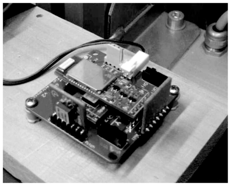
Gyroscope Hardware.

A vast literature exists on the attitude (orientation) estimation problem in the satellite guidance and control literature. In addition to those works mentioned above, see e.g., refs. [26–28,30,31,35,39,40,42–44], or almost any recent issue of the Journal of Guidance Control and Dynamics for up-to-date approaches to this problem. For a geometric approach to the problem, see ref. [41].

6.1. Model formulation

In this subsection we consider an estimation problem on SO(3) that was introduced in refs. [46,47]. Consider a rigid object with orientation that changes in time, e.g., a satellite or airplane. It is a common problem to use on-board sensors to estimate the orientation of the object at each instant in time. We now examine several models.

Let R(t) ∈ SO(3) denote the orientation of a frame fixed in the body relative to a frame fixed in space at time t. From the perspective of the rotating body, the frame fixed in space appears to have the orientation $R^{\prime }(t)\triangleq R^T(t)$. The angular velocity of the body with respect to the space-fixed frame at time t as seen in the space-fixed frame will be ω_L = vect(ṘR^T), and the same angular velocity as seen in the rotating frame will be ω_R = R^Tω_L = vect(R^T Ṙ) where Ṙ = dR/dt. These are also easily rewritten in terms of R′.

If again {X_i} denotes the set of basis elements of the Lie algebra so(3), then

$$dR(t)=\left(\sum _{i=1}^3({\mathit{\omega }}_L·{\mathbf{e}}_{i}dt)X_i\right)R(t)$$

and

$$dR(t)=R(t)\left(\sum _{i=1}^3({\mathit{\omega }}_R·{\mathbf{e}}_{i}dt)X_i\right).$$

In practice, the increments du_i = ω_R · e_i dt are measured indirectly. For instance, an inertial platform (such as a gyroscope) within the rotating body is held fixed (as best as possible) with respect to inertial space. This cannot be done exactly, i.e., there is some drift of the platform with respect to inertial space. Let A ∈ SO(3) denote the orientation of the space-fixed frame relative to the inertial platform in the rotating body. If there were no drift, A would be the identity I. However, in practice there is always drift. This has been modeled as shown in ref. [46]^§§:

$$dA(t)=\left(\sum _{i=1}^3{X}_i{dW}_i(t)\right)A(t)$$ (25)

where the three-dimensional Wiener process W(t) defines the noise model.

The orientation that is directly observable is the relative orientation of the inertial platform with respect to the frame of reference fixed in the rotating body. We denote this as Q⁻¹. In terms of R and A,

$$A^{-1}=R{Q}^{-1}.$$

Therefore Q, which is the orientation of the rotating body with respect to the inertial platform, is

$$Q=AR.$$

Taking the inverse of both sides gives

$$Q^{\prime }=R^{\prime }{A}^{\prime }.$$ (26)

From the chain rule this means

$$d{Q}^{\prime }=d{R}^{\prime }{A}^{\prime }+R^{\prime }d{A}^{\prime }.$$

Substitution of (25) and the corresponding expression for dR gives

$$d{Q}^{\prime }=\left(\sum _{i=1}^3-{du}_i{X}_i\right)R^{\prime }{A}^{\prime }+R^{\prime }{A}^{\prime }\left(\sum _{i=1}^3{X}_i{dW}_i(t)\right).$$

Using (26) and defining x_i dt = −du_i, this is written as in ref. [46]:

$$d{Q}^{\prime }=\left(\sum _{i=1}^3{x}_{i}dt{X}_i\right)Q^{\prime }+Q^{\prime }\left(\sum _{i=1}^3{X}_i{dW}_i(t)\right).$$ (27)

The particular problem that we will address is the assessment of noise properties in the gyroscope from measurements. In this context, the motions of the platform will be taken to be zero, i.e., x_i = 0. The Fokker–Planck equation corresponding to this stochastic differential equation will then be of the form of (6) subject to the initial conditions ρ(R; 0) = δ(R). The noises are assumed to be correlated as

$$\langle {dW}_i(t_i){dW}_j(t_j)\rangle ={\sigma }_{ij}\delta (t_i-t_j){dt}_i{dt}_j,$$ (28)

and we do not know (and therefore seek) the values σ_ij. The diffusion constant is related to the noises as D = Σ = [σ_ij].

From sample paths of a stochastic differential equation (which correspond to experimental measurements) we will illustrate a procedure in the next sections for estimating the noise parameters D_ij that are intrinsic to the gyroscope.

6.2. Methods for determining noise parameters from measurements

In this section we explain how errors in orientational sensing or robot pose can be quantified. We first consider the case of small errors, and then large ones. This problem is relevant to all of the examples discussed in prior sections.

6.2.1. Small errors

Small errors can be handled by expanding quantities around the identity of the group of interest and linearizing. As will be shown below, this amounts to treating concentrated distributions as distributions on IRⁿ. In particular, for a probability density function on G that is highly concentrated around the identity, we can define the covariance as

$$\mathrm{\sum }={\int }_{{IR}^n}\mathbf{x}{\mathbf{x}}^{T}f(g(\mathbf{x}))d\mathbf{x}$$ (29)

where x ∈ IRⁿ are the exponential parameters for G. The justification for this kind of linearization is given in.⁷¹

The Gaussian distribution in IR^N can be defined as the solution to a diffusion equation. This definition can be extended to the context of probability densities on the rotation group and other Lie groups. Recall that given that elements of G (viewed as square matrices) are parameterized as g = g(x), differential operators analogous to partial derivatives take the form $X_i^r$.

A diffusion equation on G is then of the form in (6). For intermediate to large values of t such equations can be solved efficiently using methods from noncommutative harmonic analysis.⁶ However, for small values of t, such methods become impractical. In contrast, as is shown in the theorem below, the concentrated Gaussian distributions discussed throughout this paper provide a closed-form solution in the small t limit.

It is easy to see that the solution to the diffusion Eq. (6) with small values of Dt is a Gaussian distribution in exponential coordinates with covariance Σ = Dt. To prove this, let g ≈ I + X. Then

$$\begin{array}{l}{X}_i^{r}f(g)={\frac{df((I+X)(I+\epsilon X_i))}{d\epsilon }\mid }_{\epsilon =0}\\ =\frac{df(I+X+\epsilon X_i+\epsilon X{X}_i)}{d\epsilon }{\mid }_{\epsilon =0}.\end{array}$$

If we define f̃(x) = f(I + X), then

$$X_i^r\stackrel{\sim }{f}\approx {\frac{d\stackrel{\sim }{f}(\mathbf{x}+\epsilon {\mathbf{e}}_i)}{d\epsilon }\mid }_{\epsilon =0}=\frac{\partial \stackrel{\sim }{f}}{\partial x_i},$$

where the approximate equality holds since both ε and ||x|| are small and so their product can be viewed as a second-order term.

The solution to Eq. (6) for small values of time (therefore resulting in a highly concentrated distribution centered around the identity) is exactly the same as the solution to

$$\frac{\partial f}{\partial t}=\frac{1}{2}\sum _{k,l=1}^n{D}_{lk}\frac{{\partial }^{2}f}{\partial x_k\partial x_l}.$$

The solution to this is well known, and is the Gaussian in IRⁿ with

$$\mathrm{\sum }=tD.$$

Therefore, for small measurement errors, we can obtain the noise properties by taking experimental measurements in the group, computing their relation with respect to a group mean of the measurements (see ref. [6] for definition of group means) and computing the covariance in exponential coordinates of the residual orientations relative to the mean:

$${\mathrm{\sum }}_{\mathit{exp}}=\frac{1}{N}\sum _{i=1}^N{\mathbf{x}}_i{\mathbf{x}}_i^T.$$

This then defines the error in the measurements on the group.

6.2.2. Large errors

For large orientational errors (i.e., those greater than 20%), the linearized analysis of the previous subsection lose their effectiveness, and other techniques are required. Fourier Density estimation is a technique to describe errors in this case.

Due to the operational property of the group Fourier transform, in SO(3) case, the Fokker–Planck equation in (6) can be written in Fourier space as

$$\frac{d{\widehat{f}}^l}{dt}={\widehat{D}}^l{\widehat{f}}^l\text{with}{\widehat{f}}^l(0)=I_{2l+1},$$

where

$${\widehat{D}}^l=\sum _{i,j=1}^3{D}_{ij}{u}^l(X_i)u^l(X_i).$$

The solution of the Fourier transform is then

$${\widehat{f}}^l=exp(t{\widehat{D}}^l).$$

This can be matched to the SO(3) Fourier transform of experimental measurements at time t in each sample path in an ensemble of N trials:

$${\widehat{f}}_{\mathit{exp}}^l(t)=\frac{1}{N}\sum _{i=1}^N{U}^l\left(R_i^{-1}(t)\right).$$

Two natural ways to perform this match are: (1) to perform a gradient descent on the six unknown diffusion parameters in the cost function

$$C_1(\{D_{ij}\},t)={\left|\right|exp(t{\widehat{D}}^l)-{\widehat{f}}_{\mathit{exp}}^l(t)\left|\right|}^2,$$ (30)

or, (2) to find in closed form the diffusion parameters by minimizing the quadratic cost function

$$C_2(\{D_{ij}\},t)={\Vert t\sum _{i,j=1}^3{D}_{ij}{u}^l(X_i)u^l(X_i)-log{\widehat{f}}_{\mathit{exp}}^l(t)\Vert }^2.$$ (31)

In practice, we solve for the minimum of C₂ and use it as the starting point for a few gradient descent iterations in the minimization of C₁. This can be done at each value of t. The answer can then be averaged over time.

6.3. Numerical experiments and results

To evaluate the methods purposed in Section 6.2.1. and 6.2.2., random samples of SO(3) need to be drawn from a known time-evolving PDF that simulates the error in a orientational rate measurement sensor. This can be done by a Monte Carlo approach and applying the Euler–Maruyama method which was introduced and explained in detail by Higham as a numerical method for SDEs.⁶⁶ With the Euler–Maruyama method, a sample value of angular velocity vector ω(t) at time t can be calculated in principle by doing numerical integration along a discretized Brownian path in the following form:

$$\mathit{\omega }(t)dt=Bd\mathbf{W}(t)$$ (32)

where W denotes a vector of unit uncorrelated Wiener processes, B is a coupling and amplification matrix, and we take as the initial condition ω(0) = [0, 0, 0]^T. However, direct integration of this angular velocity will lead to errors. Therefore, the exponential parameterization for SO(3) is used, where we write

$$\mathit{\omega }=J_r(\mathbf{x})\stackrel{.}{\mathbf{x}}.$$

Then (32) becomes:

$$d\mathbf{x}(t)=J_r^{-1}(\mathbf{x}(t))Bd\mathbf{W}(t)$$ (33)

where

$$J_r^{-1}(\mathbf{x}(t))=I_{3\times 3}+\frac{1}{2}X(t)+\left(\frac{1}{{\left|\right|\mathbf{x}(t)\left|\right|}^2}-\frac{1+cos\left|\right|\mathbf{x}(t)\left|\right|}{2\left|\right|\mathbf{x}(t)\left|\right|sin\left|\right|\mathbf{x}(t)\left|\right|}\right)X{(t)}^2.$$

Once the random samples of SO(3) are produced, the method introduced in Section 6.2.1. can be applied in small error case. The computed covariance, Σ_exp, in exponential coordinates of the sample data is then the estimate of the model covariance D_model = BB^T. To assess the accuracy of the estimate, the error in the covariance estimate

$$e=\frac{\left|\right|{\mathrm{\sum }}_{\mathit{exp}}-D_{\mathit{model}}\left|\right|}{\left|\right|D_{\mathit{model}}\left|\right|}$$

is used as a measurement of the distance (error) between the estimation and the model covariance. Note that this is not the error in the sensor, but the error in the estimation algorithm used to assess the error in the orientational rate sensor (which is defined by the covariance/diffusion matrix). Here ||·|| is the Hilbert–Schmidt (Frobenius) norm. Figure 10 shows error plot with different sample sizes. It clearly shows that the method provides a better estimate as the sample size grows for small errors.

Fig. 10.

Error plot for covariance in small errors case.

In large errors case, two methods purposed in Section 6.2.2. are tested with different configuration of B and sample sizes. Figure 11 shows the error plots for one set of configuration of B with sample sizes of 1000, 5000, 10000, and 50000. The errors is the form of $\frac{\left|\right|D_{\mathit{exp}}-D_{\mathit{model}}\left|\right|}{\left|\right|D_{\mathit{model}}\left|\right|}$ which measures the accuracy of the estimates. The x-axis represents L, the dimension of IURs (U(g) is a 2L + 1 × 2L + 1 matrix). The line with dots is the error for the method using gradient descent and the line with circles is the error for the method (2) which finds the diffusion parameters by minimizing (31). The figure shows that the larger sample size being used in the methods the better estimate one can get. The figure also indicates that the gradient descent method has better performance in terms of reducing errors. But it is very much dependent on a good choice of starting point. In practice, we can solve for the minimum of C₂ (31) and use it as the starting point.

Fig. 11.

Error plots for large errors.

7. Conclusions

We showed that irreducible unitary representation (IUR) matrices for SO(3) and SE(2) can be computed by matrix exponentiation. These IURs are used to estimate probability density functions (PDFs) via the group Fourier transforms and inversion formulae. Such PDFs arise both in applications in which physical systems are subject to noise, as well as in planning problems in which the injection of artificial noise serves as a useful tool to search configuration space.

We applied several other methods for obtaining PDFs for the stochastic kinematic cart. For the small diffusion system, the shifted Gaussian could be used for the PDF. In order to solve the path planning problem in the case with an obstacle, the sample paths were used to estimate the PDF. By the Euler–Maruyama method, we integrated the SDE to generate an ensemble of paths. By excluding the paths intersecting with the obstacle, we can take the obstacle into account when estimating the PDF. From the paths, we generated the PDF in two different ways: (1) Assigning the small Gaussian to each sample path and averaging them; (2) computing the mean and covariance from the paths and approximating the PDF by a Gaussian function with the computed mean and covariance. The PDFs were used for path planning of the kinematic cart. We also applied the shifted Gaussian method to the flexible needle to obtain the PDF and solved the path planning problem.

Detail techniques are also provided on applications of quantifying the small or large errors in orientational sensing, such as gyroscopes. This new computational tool provide us an efficient and robust density estimator on rotational groups.

References

- 1.Titterton DH, Weston JL. Strapdown Inertial Navigation Technology. Peter Peregrinus Ltd; London, UK: 1997. [Google Scholar]
- 2.Lawrence A. Modern Inertial Technology. Springer-Verlag; New York, USA: 1993. [Google Scholar]
- 3.Jekeli C. Inertial Navigation Systems with Geodetic Applications. Walter de Gruyter; Berlin; New York: 2001. [Google Scholar]
- 4.Makadia A, Daniilidis K. Rotation estimation from spherical images. IEEE Trans Pattern Anal Mach Intell. 2006;28:1170–1175. doi: 10.1109/TPAMI.2006.150. [DOI] [PubMed] [Google Scholar]
- 5.Bayro-Corrochano E, Zang Y. The motor extended Kalman filter a geometric approach for rigid motion estimation. J Math Imaging and Vis. 2000;13:205–228. [Google Scholar]
- 6.Chirikjian GS, Kyatkin AB. Engineering Applications of Noncommutative Harmonic Analysis. CRC Press; Boca Raton, FL: 2001. [Google Scholar]
- 7.Gelfand IM, Minlos RA, Ya Shapiro Z. Representations of the Rotation and Lorentz Groups and their Applications. Macmillan; New York: 1963. [Google Scholar]
- 8.Gurarie D. Symmetry and Laplacians: Introduction to Harmonic Analysis, Group Representations and Applications. Elsevier Science Publisher; The Netherlands: 1992. [Google Scholar]
- 9.Mackey GW. The Theory of Unitary Group Representations. The University of Chicago Press; Chicago: 1976. [Google Scholar]
- 10.Maslen DK. PhD Dissertation. Department of Mathematics, Harvard University; May, 1993. Fast Transforms and Sampling for Compact Groups. [Google Scholar]
- 11.Maslen DK, Rockmore DN. Generalized FFTs—a survey of some recent results. DIMACS Series Discrete Math Theor Comput Sci. 1997;28:183–237. [Google Scholar]
- 12.Miller W. Lie Theory and Special Functions. Academic Press; New York: 1968. [Google Scholar]
- 13.Miller W., Jr Some applications of the representation theory of the Euclidean group in three-space. Commun Pure App Math. 1964;17:527–540. [Google Scholar]
- 14.Naimark MA. Linear Representations of the Lorentz Group. Macmillan; New York: 1964. [Google Scholar]
- 15.Peter F, Weyl H. Die Vollständigkeit der primitiven Darstellungen einer geschlossenen kontinuierlichen Gruppe. Math Ann. 1927;97:735–755. [Google Scholar]
- 16.Sugiura M. Unitary Representations and Harmonic Analysis. 2. North-Holland, Amsterdam: 1990. [Google Scholar]
- 17.Taylor ME. Noncommutative Harmonic Analysis. Mathematical Surveys and Monographs, American Mathematical Society; Providence, RI: 1986. [Google Scholar]
- 18.Varshalovich DA, Moskalev AN, Khersonskii VK. Quantum Theory of Angular Momentum. World Scientific; Singapore: 1988. [Google Scholar]
- 19.Vilenkin NJ, Klimyk AU. Representation of Lie Groups and Special Functions. 1–3. Kluwer Academic Publishers; Dordrecht, Holland: 1991. [Google Scholar]
- 20.Wigner E. On Unitary Representations of the Inhomogeneous Lorentz Group. Ann Math. 1939;40(1):149–204. [Google Scholar]
- 21.Zelobenko ĎP. Translations of Mathematical Monographs. American Mathematical Society; Providence, RI: 1973. Compact Lie Groups and their Representations. [Google Scholar]
- 22.Kim PT. Deconvolution density estimation on SO(N) Ann Stat. 1998;26(3):1083–1102. [Google Scholar]
- 23.Silverman BW. Kernel density estimation using the fast Fourier transform. Appl Stat. 1982;31:93–99. [Google Scholar]
- 24.Hendriks H. Nonparametric estimation of a probability density on a Riemannian manifold using Fourier expansions. Ann Stat. 1990;18(2):832–849. [Google Scholar]
- 25.Silverman BW. Density Estimation for Statistics and Data Analysis. Chapman and Hall; London: 1985. [Google Scholar]
- 26.Aramanovitch LI. Quaternion nonlinear filter for estimation of rotating body attitude. Math Methods Appl Sci. 1995;18(15):1239–1255. [Google Scholar]
- 27.Bar-Itzhack IY, Oshman Y. Attitude determination from vector observations—quaternion estimation. IEEE Trans Aerosp Electron Syst. 1985;21(1):128–136. [Google Scholar]
- 28.Bar-Itzhack IY, Idan M. Recursive attitude determination from vector observations—Euler angle estimation. J Guid Control Dyn. 1987;10(2):152–157. [Google Scholar]
- 29.Burns WK, editor. Optical Fiber Rotation Sensing. Academic Press; Boston: 1994. [Google Scholar]
- 30.Carta DG, Lackowski DH. Estimation of orthogonal transformations in strapdown inertial systems. IEEE Trans Autom Control. 1972;AC-17:97–100. [Google Scholar]
- 31.Chaudhuri S, Karandikar SS. Recursive methods for the estimation of rotation quaternions. IEEE Trans Aerosp Electron Syst. 1996;32(2):845–854. [Google Scholar]
- 32.Comisel H, Forster M, Georgescu E, Ciobanu M, Truhlik V, Vojta J. Attitude estimation of a near-earth satellite using magnetometer data. Acta Astronautica. 1997;40(11):781–788. [Google Scholar]
- 33.Crassidis JL, Lightsey EG, Markley FL. Efficient and optimal attitude determination using recursive global positioning system signal operations. J Guid Control Dyn. 1999;22(2):193–201. [Google Scholar]
- 34.Crassidis JL, Markley FL. Predictive filtering for attitude estimation without rate sensors. J Guid Control Dyn. 1997;20(3):522–527. [Google Scholar]
- 35.Lefferts EJ, Markley FL, Shuster MD. Kalman filtering for spacecraft attitude estimation. J Guid Control Dyn. 1982;5(5):417–429. [Google Scholar]
- 36.Duncan TE. An Estimation problem in compact Lie groups. Syst Control Lett. 1998;10:257–263. [Google Scholar]
- 37.Lo JT-H, Eshleman LR. Exponential Fourier densities on SO(3) and optimal estimation and detection for rotational processes. SIAM J Appl Math. 1979;36(1):73–82. [Google Scholar]
- 38.Lo JTH. Optimal estimation for the satellite attitude using star tracker measurements. Automatica. 1986;22(4):477–482. [Google Scholar]
- 39.Oshman Y, Markley FL. Minimal-parameter attitude matrix estimation from vector observations. J Guid Control Dyn. 1998;21(4):595–602. [Google Scholar]
- 40.Oshman Y, Markley FL. Sequential attitude and attitude-rate estimation using integrated-rate parameters. J Guid Control Dyn. 1999;22(3):385–394. [Google Scholar]
- 41.Park FC, Kim J, Kee C. Geometric descent algorithms for attitude determination using the global positioning system. J Guid Control Dyn. 2000;23(1):26–33. [Google Scholar]
- 42.Savage PG. Strapdown inertial navigation integration algorithm design part 1: Attitude algorithms. J Guid Control Dyn. 1998;21(1):19–28. [Google Scholar]
- 43.Savage PG. Strapdown inertial navigation integration algorithm design part 2: Velocity and position algorithms. J Guid Control Dynamics. 1998;21(2):208–221. [Google Scholar]
- 44.Shuster MD, Oh SD. Three-axis attitude determination form vector observations. J Guid Control Dyn. 1981;4(1):70–77. [Google Scholar]
- 45.Smith RB, editor. SPIE Milestone Series. MS 8. SPIE Optical Engineering Press; Washington, DC: 1989. Fiber Optic Gyroscopes. [Google Scholar]
- 46.Willsky AS. Some Estimation Problems on Lie Groups. In: Mayne DQ, Brockett RW, editors. Geometric Methods in System Theory. Reidel Publishing Company; Dordrecht-Holland: 1973. pp. 305–313. [Google Scholar]
- 47.Willsky AS. PhD Dissertation. Department of Aeronautics and Astronautics, MIT; 1973. Dynamical Systems Defined on Groups: Structural Properties and Estimation. [Google Scholar]
- 48.Moses HE. Irreducible representations of the rotation group in terms of the axis and angle of rotation. Ann Phys. 1967;42:343–346. [Google Scholar]
- 49.Moses HE. Irreducible representations of the rotation group in terms of the axis and angle of rotation. Ann Phys. 1966;37:224–226. [Google Scholar]
- 50.Moses HE. Irreducible representations of the rotation group in terms of Euler’s theorem. Il Nuovo Cimento. 1965;40(4):1120–1138. [Google Scholar]
- 51.Applebaum D, Kunita H. Lévy flows on manifolds and Lévy processes on Lie groups. J Math Kyoto Univ. 1993;33/34:1103–1123. [Google Scholar]
- 52.Brockett RW. Notes on Stochastic Processes on Manifolds. In: Byrnes CI, et al., editors. Systems and Control in the Twenty-First Century. Birkhäuser; Boston: 1997. pp. 75–101. [Google Scholar]
- 53.Fokker AD. Die Mittlere Energie rotierender elektrischer Dipole in Strahlungs Feld. Ann Physik. 1914;43:810–820. [Google Scholar]
- 54.Gardiner CW. Handbook of Stochastic Methods. 2. Springer-Verlag; Berlin: 1985. [Google Scholar]
- 55.Itô K. Brownian Motions in a Lie Group. Proceedings of the Japan Academy. 1950;26:4–10. [Google Scholar]
- 56.Itô K. Stochastic differential equations in a differentiable manifold. Nagoya Math J. 1950;1:35–47. [Google Scholar]
- 57.Itô K. Stochastic differential equations in a differentiable manifold (2) Sci Univ Kyoto Math, Series A. 1953;28(1):81–85. [Google Scholar]
- 58.Kunita H. Stochastic Flows and Stochastic Differential Equations. Cambridge University Press; Cambridge, UK: 1997. [Google Scholar]
- 59.McConnell J. Rotational Brownian Motion and Dielectric Theory. Academic Press; New York: 1980. [Google Scholar]
- 60.McKean HP., Jr Brownian motions on the 3-dimensional rotation group. Mem Coll Sci Univ Kyoto, Series A. 1960;33(1):2538. [Google Scholar]
- 61.Planck M. Uber einen Satz der statistischen Dynamik und seine Erweiterung in der Quantentheorie. Sitz ber Berlin A Akad Wiss. 1917;1917:324–341. [Google Scholar]
- 62.Risken H. The Fokker–Planck Equation, Methods of Solution and Applications. 2. Springer-Verlag; Berlin: 1989. [Google Scholar]
- 63.Roberts PH, Ursell HD. Random walk on a sphere and on a Riemannian manifold. Phil Trans R Soc London. 1960;A252:317–356. [Google Scholar]
- 64.van Kampen NG. Stochastic Processes in Physics and Chemistry. North Holland, Amsterdam: 1981. [Google Scholar]
- 65.Yosida K. Integration of Fokker–Planck’s equation in a compact Riemannian space. Arkiv für Matematik. 1949;1(9):71–75. [Google Scholar]
- 66.Higham DJ. An algorithmic introduction to numerical simulation of stochastic differential equations. SIAM Rev. 2001;43(3):525–546. [Google Scholar]
- 67.Murray RM, Li Z, Sastry SS. A Mathematical Introduction to Robotic Manipulation. CRC Press; Ann Arbor MI: 1994. [Google Scholar]
- 68.Smith P, Drummond T, Roussopoulos K. Computing MAP Trajectories by Representing, Propagating and Combining PDFs over Groups. Proceedings of the 9th IEEE International Conference on Computer Vision; Nice, France. 2003; pp. 1275–1282. [Google Scholar]
- 69.Su S, Lee CSG. Manipulation and propagation of uncertainty and verification of applicability of actions in assembly tasks. IEEE Trans Syst Man Cybern. 1992;22(6):1376–1389. [Google Scholar]
- 70.Zhou Y, Chirikjian GS. Probabilistic Models of Dead-Reckoning Error in Nonholonomic Mobile Robots. Proceedings of ICRA’03; Taipei, Taiwan. Sep. 14–19, 2003; pp. 1594–1599. [Google Scholar]
- 71.Wang Y, Chirikjian GS. Error propagation on the Euclidean group with applications to manipulator kinematics. IEEE Trans Robot. 2006;22(4):591–602. [Google Scholar]
- 72.Wang Y, Chirikjian GS. Worksapce generation of hyper-redundant manipulators as a diffusion process on SE(N) IEEE Trans Robot Autom. 2004;20(3):339–408. [Google Scholar]
- 73.Wang Y, Chirikjian GS. A New Potential Field Method for Robot Path Planning. Proceedings of ICRA’00; San Francisco, CA . Apr. 2000; pp. 977–982. [Google Scholar]
- 74.Choset H, Burgard W, Hutchinson S, Kantor G, Kavraki LE, Lynch K, Thrun S. Principles of Robot Motion: Theory, Algorithms, and Implementation. MIT Press; Cambridge, MA, USA: 2005. [Google Scholar]
- 75.Chirikjian GS, Ebert-Uphoff I. Numerical convolution on the Euclidean group with applications to workspace generation. IEEE Trans Robot Autom. 1998;14(1):123–136. [Google Scholar]
- 76.Ebert-Uphoff I, Chirikjian GS. Inverse Kinematics of Discretely Actuated Hyper-Redundant Manipulators Using Workspace Densities. Proceedings of ICRA’96; Minneaoplis, MN. Minneapolis, MN, USA: pp. 139–145. [Google Scholar]
- 77.Mason R, Burdick JW. Trajectory Planning Using Reachable-State Density Functions. 2002 IEEE International Conference on Robotics and Automation; Washington, DC. May 2002; pp. 273–280. [Google Scholar]
- 78.Kyatkin AB, Chirikjian GS. Computation of robot configuration and workspaces via the Fourier transform on the discrete motion group. Int J Robot Res. 1999;18(6):601–615. [Google Scholar]
- 79.Li Z, Canny JF, editors. Nonholonomic Motion Planning. Kluwer Academic Publishers; Dordrecht, The Netherlands: 1993. [Google Scholar]
- 80.Laumond J-P, editor. Robot Motion Planning and Control. Springer; New York, USA: 1998. [Google Scholar]
- 81.Chirikjian GS, Burdick JW. A modal approach to hyper-redundant manipulator kinematics. IEEE Trans Robot Autom. 1994;10:343–54. [Google Scholar]
- 82.Webster RJ, III, Kim JS, Cowan NJ, Chirikjian GS, Okamura AM. Nonholonomic modeling of needle steering. Int J Robot Res. 2006;25:509–525. [Google Scholar]
- 83.Park W, Kim JS, Zhou Y, Cowan NJ, Okamura AM, Chirikjian GS. Diffusion-Based Motion Planning for a Nonholonomic Flexible Needle Model. IEEE International Conference on Robotics and Automation; 2005; Barcelona, Spain. pp. 4611–4616. [Google Scholar]
- 84.Alterovitz R, Simeon T, Goldberg K. The stochastic motion roadmap: A sampling framework for planning with Markov motion uncertainty. Proc. Robotics: Science and Systems III; June 2007; Atlanta, CA. [Google Scholar]