A CROC stronger than ROC: measuring, visualizing and optimizing early retrieval

Abstract

Motivation: The performance of classifiers is often assessed using Receiver Operating Characteristic ROC [or (AC) accumulation curve or enrichment curve] curves and the corresponding areas under the curves (AUCs). However, in many fundamental problems ranging from information retrieval to drug discovery, only the very top of the ranked list of predictions is of any interest and ROCs and AUCs are not very useful. New metrics, visualizations and optimization tools are needed to address this ‘early retrieval’ problem.

Results: To address the early retrieval problem, we develop the general concentrated ROC (CROC) framework. In this framework, any relevant portion of the ROC (or AC) curve is magnified smoothly by an appropriate continuous transformation of the coordinates with a corresponding magnification factor. Appropriate families of magnification functions confined to the unit square are derived and their properties are analyzed together with the resulting CROC curves. The area under the CROC curve (AUC[CROC]) can be used to assess early retrieval. The general framework is demonstrated on a drug discovery problem and used to discriminate more accurately the early retrieval performance of five different predictors. From this framework, we propose a novel metric and visualization—the CROC(exp), an exponential transform of the ROC curve—as an alternative to other methods. The CROC(exp) provides a principled, flexible and effective way for measuring and visualizing early retrieval performance with excellent statistical power. Corresponding methods for optimizing early retrieval are also described in the Appendix.

Availability: Datasets are publicly available. Python code and command-line utilities implementing CROC curves and metrics are available at http://pypi.python.org/pypi/CROC/

Contact: pfbaldi@ics.uci.edu

1 INTRODUCTION

One of the most widely used tools to assess the performance of a classification or ranking algorithm in statistics and machine learning is the Receiver Operating Characteristic (ROC) curve, plotting true versus false positive rate, together with the corresponding area under the ROC curve (AUC[ROC]) metric. However, in many applications, ranging from information retrieval to drug discovery, the ROC curve and the area under the curve (AUC) metric are not very useful. This is because the total number of objects to be classified or ranked, such as web pages or chemical molecules, tends to be very large relative to the number of objects toward the top of the list that are practically useful or testable due to, for instance, financial constraints. Specifically, consider a typical drug discovery situation where one is interested in discovering molecules that may be ‘active’ among a library of 1 000 000 molecules by computational virtual screening methods, such as docking or similarity search. Depending on the financial conditions and the details of the corresponding experimental setup, experimentalists may be able to test in the laboratory, for instance, only the top 1000 hits on the list. In such conditions, the majority of the ROC curve is without much relevance and the AUC is useless. Only the early portion of the ROC curve is relevant. Furthermore, the precise ranking of the molecules, particularly for the bottom 999 000 molecules, is also of very minor interest. Similar observations can be made in many other areas, ranging from fraud detection to web page retrieval. What one is really interested in across all these cases is the notion of early enrichment/recognition/retrieval, having as many true positives as possible within the list of top hits.

To further drive this point, consider the following three cases from Truchon and Bayly (2007) corresponding to an algorithm that either: (1) ranks half the positive candidates at the top of the list and half at the bottom; (2) distributes the positive candidates uniformly throughout the list; or (3) ranks all the positive candidates exactly in the middle of the list. All three cases yield an AUC of 0.5 although, if only the top few hits can be experimentally tested, Case 1 is clearly better than Case 2 which, in turn, is better than Case 3. Good early recognition metrics and visualization tools ought to easily discriminate between these cases and rank them appropriately.

Several metrics have been suggested in the literature to address the early retrieval problem, but none seems entirely satisfactory. Some metrics lack smoothness and require setting arbitrary thresholds, including looking at the derivative of the smoothed ROC curve at or near the origin, or looking at the ROC curve and its area over the interval [0, t] for some threshold t (e.g. t = 0.05). However, as we shall see, methods with hard threshold cutoffs tend to be less statistically powerful than methods without threshold cutoffs, because they discard meaningful differences in the performance of the classifiers just beyond the cutoff threshold. Other interesting metrics that explicitly try to avoid setting an arbitrary threshold (Clark and Webster-Clark, 2008; Sheridan et al., 2001; Truchon and Bayly, 2007) have other limitations, such as being untunable, lacking good visualization or generality, or requiring the non-principled choice of a transformation (see Section 6).

In this article, the early retrieval problem is addressed by introducing and studying a general framework—the concentrated ROC (CROC) framework—for both measuring and visualizing early retrieval performance in a principled way that is more suitable than the ROC curve and the AUC measure. The overall approach is demonstrated on a drug discovery problem. Finally, CROC is discussed in relation to other metrics in the literature and shown to provide a general unifying framework. Methods for maximizing early retrieval performance are described in the Appendix A.

2 THE CROC FRAMEWORK

2.1 The ROC

Classification (or ranking) performance can be assessed using single-threshold metrics. For a given threshold, the number of true positives (TP), true negatives (TN), false positives (FP) and false negatives (FN) can be used to compute quantities such as sensitivity, specificity, precision, recall and accuracy (e.g. Baldi et al., 2000). Measuring performance at a single threshold, however, is somewhat arbitrary and unsatisfactory. To obviate this problem and capture performance across multiple thresholds, it is standard to use ROC or AC (accumulation curve or enrichment curve) curves and the area under these curves. The ROC curve plots the TP rate (TPR), as a function of the FP rate (FPR). The AC plots the TP rate as a function of the FDP, the fraction of the data classified as positive at a given threshold, and is occasionally used to assess virtual screening methods (Seifert, 2006). The ROC curve and AC are related by a linear transformation of the x-axis. The area under the ROC curve (AUC[ROC]) or area under the AC (AUC[AC]) can be used to quantify global performance. The AUC[AC] is a linear transform of the AUC[ROC] and the two metrics are approximately equivalent as the size of the dataset increases (Truchon and Bayly, 2007).

Within the ROC or AC framework, a classifier can be assessed by comparing its performance to the performance of a random classifier, or to the best possible and worst possible classifiers. The random classifier corresponds to an algorithm that randomly and uniformly distributes all the positive candidates throughout its prediction-sorted list. This is exactly equivalent to using a random number generator, uniform in [0, 1], to produce class membership probabilities. For both the ROC and AC plots, averaging the performance curves of a large number of random trials of a random classifier constructed in this manner yields a straight line from the origin to the point (1, 1), with an area 0.5. Classifiers worse than random, therefore, yield an AUC[ROC] <0.5. Furthermore, the variance of the random AUC[ROC] or AUC[AC] can be estimated analytically or by Monte Carlo simulations and used, for instance, to derive a Z-score for the area. The best and worst classifiers assume that all the positive candidates are ranked at the top or bottom, respectively, of the prediction sorted list. These also provide a useful baseline, especially for visualization of the AC curve by providing extreme curve boundaries. Masking out the portion of the plot above the best possible curve and below the worst possible curve highlights the region within which the AC curve is confined (Fig. 1).

Fig. 1.

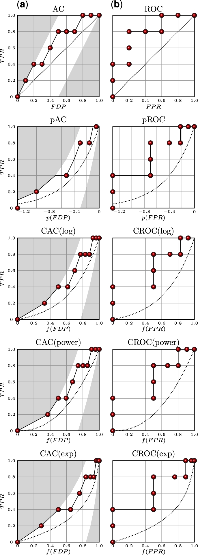
Different performance curves for a dataset with 10 instances and positives ranked 1, 2, 4, 5 and 8 by a hypothetical prediction algorithm. (a) AC curves. (b) ROC curves. pAC and pROC use a logarithmic transformation described in Clark and Webster-Clark (2008) (see Section 6). For each row from the top, the x-coordinates are: (i) untransformed; (ii) transformed by logarithmic equation f(x) = log₁₀(max[x, 0.5/N]); (iii) transformed by logarithmic equation f(x) = log(1 + αx)/log(1 + α); (iv) transformed by power equation f(x) = x^[1/(1+α)]; and (v) transformed by exponential equation f(x) = (1−e^−αx)/ (1−e^−α). α is the global magnification factor and N the total number of examples. α is chosen so that f(0.1) = 0.5. For AC curves, areas above the best and below the worst possible curves are shaded. Dotted lines represent the performance of the random classifier.

However, despite their usefulness, the ROC and AC curves and their AUCs measure and visualize classification performance uniformly across the entire data, and therefore are poorly suited to measure and visualize early retrieval performance. Thus, to address this shortcoming, we next introduce the CROC framework using ROC curves as the starting point, but similar ideas apply immediately to AC curves.

2.2 The CROC

Here, we propose a different approach whereby any portion of the ROC curve of interest is magnified smoothly using an appropriate continuous and monotone (hence one to one) function f from [0, 1] to [0, 1], satisfying f(0) = 0 and f(1) = 1. Since this general approach tends to concentrate resources on a particular portion of the ROC curve, we call it the Concentrated ROC (CROC) approach [and concentrated AC (CAC)]. The approach can be used to magnify the x- axis or the y-axis, or both. Here, we focus primarily on magnification along the x-axis, since this is the most critical in early retrieval, but the same ideas can be applied to the y-axis if necessary. Since we are interested in the early portion of the ROC curve, we need a function that expands the early part of the [0,1] interval, and contracts the latter part. This is easily achieved using a function f that is concave down (∩), i.e with a negative second derivative in the differentiable case. Many such functions are possible and it is reasonable to further require that such functions have a simple expression, with at most one parameter to control the overall level of magnification. Examples of natural choices for the function f, using exponential, power, or logarithmic representations include

(1)

where α > 0 is the global magnification factor. The logarithmic transformation f(x) = [log₂(1 + x)]^1/(α+1) is also possible but yields curves that are fairly similar to the power transformation above, as can be seen with a Taylor expansion. Of course, the common technique of displaying the initial portion of the ROC curve is equivalent to using the transform function

(2)

where t = 1/(1 + α) is the hard threshold cutoff after which the ranks of positive instances are ignored. For all these transformations, at a given point x, the derivative f′(x) measures the local degree of magnification: a small interval of length dx near x is transformed into an interval of length f′(x)dx. If f′(x) > 1, the region around x is being stretched. If f′(x) < 1, the region around x is being contracted. Thus, the functions under consideration magnify the early part of the x-axis until the point where f′(x) = 1 where there is no magnification. Past this point, the functions contract the x-axis. In contrast, the threshold cutoff function of Equation (2) corresponds to a constant magnification factor of 1/t over [0, t].

2.3 Choice of magnification curve and parameters

The choice of magnification curve f and magnification parameter α can be done using additional considerations, such as ‘user behavior’. For instance, in a web page retrieval application, one may know on average how often the first, second, third, …records are clicked. The corresponding decreasing curve of how relevant each rank is provides valuable information for the range and magnification levels required. While it is possible to use the empirical relevance levels recorded in a particular application, for a more principled approach here we can imagine that this relevance g(r/N) decays exponentially or as a power law, as a function of the rank r (the scaling factor N is the total number of examples). Thus g(r/N)=Ce^−βr/N or g(r/N)=C/(r/N)^β+1, with β>0. It is reasonable to require the local magnification factor to be proportional to the corresponding relevance so that

(3)

for some proportionality constant D, so that f(x)=DG(x)+K, where G is a primitive of g and K is another constant. In the exponential and power-law cases, Equation (3) can be solved exactly taking into account the boundary values f(0)=0 and f(1)=1. When g decays exponentially, a simple calculation yields precisely the magnification function thus α=β. When g decays like a power law, one obtains precisely f(x)=x^−β thus α=β−1. Thus, in short, the magnification function can be derived precisely from the relevance function.

In the application to be considered, an exponentially decaying relevance fits well with the drug discovery setting. Thus, in the rest of the paper, for both theoretical and practical reasons we use the exponential transformation f=(1−e^−αx)/(1−e^−α) with magnification factor α. The same ideas, however, can be applied immediately with any other transformation.

For setting the parameter α, several strategies can be used. Solving f′(x)=1 yields the point x₁ where the local magnification is 1. For the exponential transformation, this gives

(4)

the approximation being valid for large values of α. Alternatively, one could choose α to sensibly map a particular value of x to another one [e.g. f(0.1)=0.5], or to match other particular conventions (e.g. α=20 in the exponential case corresponds roughly to 8% enrichment).

2.4 Area under the CROC curve (AUC[CROC]) and random classifiers

The early recognition performance of a classifier can be measured by the AUC[CROC]. This area depends on the magnification factor α, and therefore both the area and α must be reported. Under smoothness assumptions, it can be shown by Taylor expanding the ROC function, that in the limit of very large α the AUC[CROC] goes to 0 like ROC'(0)/α, where ROC'(0) represents the derivative of the ROC curve at the origin. Note that if both the x and y axes are magnified with the same transform using the same α, then the limit is ROC'(0). Thus, asymptotically the AUC[CROC] depends on the tangent of the ROC curve at the origin, although in practice CROC curves are interesting primarily for finite values of α (see Section 5).

As for the AUC[ROC], the AUC[CROC] can also be compared to the same area computed for a random classifier. The ROC curve of a completely random classifier is the straight diagonal line y=x between the points (0, 0) and (1, 1). The CROC curve of a random classifier is easily obtained by applying the magnification function f to this line. In the case of the exponential transform, the equation of the corresponding curve is given by

(5)

This curve is approximately a line y≈x(1 − e^−α)/α when α is small. But otherwise the curve is far from being a line (see Figs 1 and 2). The AUC[ROC] of a random classifier is 0.5. The AUC[CROC]_rand of a random classifier is given by

(6)

and so it behaves like 1/α for large values of the magnification factor α.

Fig. 2.

10-fold cross-validated performance of the MAX-SIM, kNN, SVM and IRV algorithms on the HIV data displayed using: (a) standard ROC curves; (b) CROC curves with α = 7 [f(0.1) = 0.5]; (c) CROC curves with α = 14 [f(0.05) = 0.5]; and (d) CROC curves with α = 80 [f(0.0086) = 0.5], displaying the first 1 000 hits for the IRV on the first half of the curve.

2.5 Assessing significance

Assessing the statistical significance of the difference in performance between two classifiers is a fundamentally more important and general task than assessing the significance between a classifier's performance and a random classifier. In most interesting settings, several classifiers are available that clearly perform better than random. The differences in performance between these classifiers, however, can be more subtle and require statistical assessments. In simple terms, how significant is a difference in AUC[ROC] for classification or AUC[CROC] for early enrichment between two different algorithms? We propose and compare six ways of assessing the significance of the difference between two early retrieval performances: (i) an unpaired permutation test; (ii) a paired permutation test; (iii) an unpaired t-test; (iv) a paired t-test; (v) an unpaired Wilcoxon test; and (vi) a paired Wilcoxon test.

The unpaired permutation test follows from the observation that the performance of two algorithms being compared is exactly defined by the size N of the entire dataset and the exact ranks assigned by each algorithm to the positive instances in this dataset (Zhao et al., 2009). Next, the ranks of the positive instances from both algorithms are pooled together and randomly partitioned into equally sized sets of ranks. Once the ranks are sampled in this way, the difference in performance between these two randomly derived methods is computed using, for instance, AUC[ROC] or AUC[CROC]. Several samples of this difference in performance can be drawn by repeatedly partitioning the ranks and compared to the observed value of interest. Significance can be assessed by estimating a P-value corresponding to the percentage of times that the sampled differences in performance are greater than the observed difference. Enough samples must be drawn to establish the desired level of confidence in the P-value. For example, if the performance difference between algorithms A and B is 0.13, then this difference would be considered significant at a P=0.05 level if at most 50 out of 1000 sampled performance differences are >0.13.

The paired permutation test is novel in this context and computed in a nearly identical manner. The only difference is the way the ranks are partitioned. For the paired permutation test, the ranks are partitioned so as to ensure that each instance's rank is included exactly one time in each partition. This is equivalent to flipping an unbiased coin once for each instance in the dataset. If the coin comes up heads, the rank of this instance in the first algorithm's list is put in the first partition and the corresponding rank produced by the second algorithm is put in the second partition. If the coin comes up tails, these ranks are placed in the opposite partitions. Once the ranks have been partitioned, the Monte Carlo procedure is repeated a sufficient number of times to determine a corresponding P-value.

The permutation tests we have described make few assumptions about the data but do require substantial amounts of computations, especially for the reliable estimation of small P-values. A faster approach is obtained by performing the appropriate unpaired and paired t-tests. These t-tests rely on normality assumptions or approximations, which may be more or less accurate, and therefore the t-tests can be expected to be less precise than extensive permutation testing.

The t-tests are derived by observing that computing the AUC[CROC] is equivalent to computing the mean of the transformed FPRs of the positive instances. For example, if a method ranks five positive instances at ranks {1, 2, 4, 5, 7} in a list of 10 total instances, this corresponds to FPRs of {0, 0, 0.2, 0.2, 0.4} for each positive instance, and to transformed FPRs of {f(0), f(0), f(0.2), f(0.2), f(0.4)}. It can easily be seen that the AUC[CROC] is exactly the mean of {1 − f(0), 1 − f(0), 1 − f(0.2), 1 − f(0.2), 1 − f(0.4)}. From this observation, one can compute a t-test between the population of transformed FPRs produced by one classifier against the similar population produced by another classifier. This approximates the results of the unpaired permutation test. Similarly, a paired t-test between the two populations approximates the results of the paired permutation test. An even faster approximation for the unpaired case is obtained by applying the t-test using the mean and SD of each classifier's performance derived by cross-validation methods.

A parallel derivation shows that computing the AUC[CAC] is equivalent to computing the mean of the transformed ranks. Using the same example, this would correspond to computing the mean of {1 − f (0.1), 1 − f(0.2), 1 − f (0.4), 1 − f (0.5), 1 − f(0.7)}. From this observation, it is easy to see how a t-test approximation of the permutation test can be constructed for the AUC[CAC] as well.

The accuracy of the t-test approximations depend on the normality of the distribution of the transformed ranks. Clearly, the transformed ranks can be very skewed, and therefore violate the t-tests' normality assumptions. This motivates the last two significance tests implemented here, which use either a paired or unpaired Wilcoxon test on the same population of transformed ranks used for the t-tests. The Wilcoxon tests are more robust to outliers and do not make normality assumptions; however, they are not designed to analytically approximate the permutation tests.

3 DRUG DISCOVERY DATA, REPRESENTATIONS, AND SIMILARITY MEASURES

Drug discovery data: we use the benchmark dataset associated with the Drug Therapeutics Program (DTP) AIDS Antiviral Screen made available by the National Cancer Institute (NCI) (http://dtp.nci.nih.gov/docs/aids/aids_data.html). The set contains assay results for 42 678 chemicals experimentally tested for their ability to inhibit the replication of the human immunodeficiency virus in vitro. Initially, the data is divided into three classes: inactive, active and moderately active. In what follows, we combine the active and moderately active classes into a single ‘active’ class containing about 3.5% of the data. Thus, the final dataset contains 1503 active molecules and 41 175 inactive molecules. All performance metrics are computed using 10-fold cross-validation experiments.

Chemical representations: molecules are described by their labeled molecular graph, where the vertices correspond to the atoms of the molecule, labeled by the atom type [e.g. carbon (C), nitrogen (N) and oxygen (O)], and the edges correspond to the bonds connecting these atoms together, labeled by the bond type (e.g. single and double). In chemoinformatics, these variable-size molecular graphs are routinely converted into long, fixed-size, binary fingerprint vectors. Each bit in a fingerprint representation corresponds to the presence or absence of a particular feature in the molecular graph. Typical sets of features used in the literature (Hassan et al., 2006; Leach and Gillet, 2005; Swamidass and Baldi, 2007) are labeled paths up to a certain length, or labeled trees up to a certain depth. While the methods to be presented can be applied with any set of features, here we use circular substructures (Hassan et al., 2006), corresponding to labeled trees of depth up to 2. Each vertex is labeled by the atomic symbol of the corresponding atom together with the number of non-hydrogen atoms to which it is bonded (e.g. C3 for a carbon with three non-hydrogen atoms attached), and each bond is labeled according to its bond type (single, double, triple or aromatic). We choose this particular labeling scheme and set of features because the resulting representations seem to yield reasonable performance based on experiments performed using other datasets (not reported).

Chemical similarity measures: although there are several possible ways of defining similarity between fingerprint vectors (Holliday et al., 2002), by far the most widely used approach is the well-known Jaccard–Tanimoto similarity measure (Leach and Gillet, 2005). If and are the fingerprint vectors representing molecules A and B, the Jaccard–Tanimoto similarity between A and B is defined by

(7)

where A∩B is the number of 1 bits in the intersection AND , and A ∪ B is the number of 1 bits that appear in the union OR . It is well known that the Jaccard–Tanimoto similarity measure satisfies the Mercer's conditions and, hence, yields a Mercer kernel (Swamidass et al., 2005a).

4 CLASSIFIERS

In the experiments, we use the CROC framework to compare the early retrieval performance of five different classifiers: RANDOM, MAX-SIM, k-Nearest-Neighbors (kNN), support vector machine (SVM) and Influence Relevance Voter (IRV). Although the details of the algorithms are not relevant to this study, we describe them briefly for completeness. RANDOM corresponds to a random classifier, which assigns a random probability chosen uniformly over [0, 1] to each example. The maximum-similarity algorithm MAX-SIM (Hert et al., 2004, 2005) is one of the simplest methods for virtual high-throughput screening by which a molecule is scored by its highest (Tanimoto) similarity to a known active molecule. Formally, if all known active compounds are denoted by {X₁,…, X_P}, the score of a new molecule X is given by

(8)

MAX-SIM has been well studied and is straightforward to implement. However, it is a rather unrefined method, which takes very little information into account ignoring, for instance, all information about known inactive molecules. A slightly more refined method is the k-nearest-neighbor algorithm, where one scores a molecule using the fraction of its k-nearest-neighbors that are active. For the SVM algorithm, it is well known that the Tanimoto similarity satisfies Mercer's condition (Swamidass et al., 2005a), and therefore it defines a kernel that can be used in an SVM for classification (see Azencott et al., 2007; Mahé et al., 2006; Swamidass et al., 2005b, for other related kernels). Finally, we use the IRV algorithm (Swamidass et al., 2009), which can be viewed as a refinement of kNN. At a high-level, the IRV is defined by a preprocessing step, during which all the neighbors–as defined by the Tanimoto similarity metric–of a test molecule are identified, and a processing step during which information from each neighbor is fed into a neural network to produce a prediction. The prediction is computed from the ‘influence’ of each neighbor, which in turn is computed as the product of each neighbor's ‘relevance’, encoding how much each neighbor should affect the prediction, and ‘vote’, encoding the direction towards which the prediction should be pushed. The output probability of membership in the active class is computed as

(9)

where X is the test molecule, i ranges from 1 to k over all the k-nearest−neighbors, I_i the ‘influence’ of the ith neighbor on the output, w_z the bias of the output node and σ(x) the logistic function 1/(1+e^−x). These influences indicate exactly how much, and in which direction, each training example contributes to the prediction and can be used to interpret each final prediction. The influence of the ith node is defined multiplicatively by I_i = R_i(X)V_i(X), where R_i(X) is the relevance and V_i(X) is the vote of the ith neighbor. Here the relevance is defined by

(10)

where s_i is the similarity S(X, N_i) of the ith closest neighbor to the test compound, r_i the rank of the ith neighbor in the similarity-sorted list of neighbors, w_s and w_r parameters tuning the importance of different inputs, and w_y the bias of this logistic function. For this study, we define the vote by: V_i = w₀ if c_i = 0 and V_i = w₁ if c_i = 1, where w₀ is the weight associated with inactive neighbors, w₁ the weight associated with active neighbors and c_i ∈ {0, 1} the class of the ith neighbor. The IRV is trained by gradient descent on the relative entropy (or negative log-likelihood). Thus, this version of the IRV has only six tunable parameters: three parameters w_s, w_r, and w_y shared across all k neighbors, and three additional parameters, w₁, w₀, and w_z–making overfitting unlikely. In the experiments, the neighborhood parameter k is set to 20 for both the kNN and IRV algorithms.

5 RESULTS

5.1 CROC metric and visualization

First, the ROC and CROC frameworks are compared by examining how they assess the early retrieval performance of the classifiers. Figure 2a shows the ROC curves of the various classifiers on the HIV data. It is virtually impossible to disentangle their performances in terms of early recognition using the ROC curves. In contrast, Figure 2b, c and d obtained by using exponential CROC curves with different global magnification factors α, show immediately that the CROC framework disambiguates the early retrieval performance of the classifiers. In these plots, increasing magnification factors of α = 7, 14 and 80 are used, corresponding to magnification functions that send the points x = 0.1, 0.05 and 0.0086 onto x = 0.5, respectively. The value 0.0086 is chosen because it is the FPR obtained by looking at the 1000 compounds that are top-ranked by the IRV. With the magnification, it becomes immediately apparent that in this case the IRV has better early recognition performance, followed by the kNN, SVM and MAX-SIM in that order, although there is a range of low values where MAX-SIM may be slightly better than the SVM. Among the top 1000 ranked compounds, the IRV retrieves 645 positives, to be compared to 603 for the kNN and 616 for the SVM. Furthermore, the results are consistent at all magnification scales, thus the CROC approach appears to be robust with respect to the choice of α.

These visualization results are confirmed in Table 1 that displays the AUC[ROC] and AUC[CROC] of the various algorithms, for different values of α. While the SVM has a slightly better AUC[ROC] than the IRV (0.852 versus 0.845), the CROC metrics confirm the advantage of the IRV algorithm for this task in terms of early recognition, consistently across different values of α. For example, for α = 80, the IRV achieves an AUC[CROC] of 0.400 compared to 0.310 for the SVM. Although, the differences between the best methods—IRV, SVM and kNN—are small, they are significant, as demonstrated in the Section 5.2.

Table 1.

AUC[ROC] and AUC[CROC] achieved by the five classifiers obtained using 10-fold cross-validations on the HIV data

	AUC[ROC]	AUC[CROC]
		α = 7	α = 14	α = 80
RANDOM	0.500	0.142	0.071	0.013
MAXSIM	0.806 (± 0.002)	0.592 (± 0.002)	0.497 (± 0.003)	0.237 (± 0.004)
kNN	0.742 (± 0.003)	0.638 (± 0.004)	0.559 (± 0.005)	0.365 (± 0.005)
SVM	0.852 (± 0.004)	0.644 (± 0.003)	0.557 (± 0.002)	0.310 (± 0.006)
IRV	0.845 (± 0.002)	0.656 (± 0.003)	0.584 (± 0.003)	0.400 (± 0.004)

Best performances are in bold and second-best performances are in italics. SDs are in parentheses.

5.2 Assessing significance

We have applied the six proposed methods for assessing significance (paired and unpaired permutation tests, paired and unpaired t-tests, paired and unpaired Wilcoxon tests) to all the known metrics for assessing early retrieval [e.g. AUC[ROC], AUC[ROC] with hard threshold cutoff t, AUC[CROC], AUC[pROC] and Boltzman-enhanced discrimination of the ROC (BEDROC)] and to all five classifiers. For the methods with hard threshold cutoffs, the thresholds were chosen to correspond to general practice (FP = 50 corresponds to ROC50) and to the values of the magnification factor α we tested, thus t = 0.5 corresponds to α = 7, t = 0.1 corresponds to α = 14 and t = 0.0086 corresponds to α = 80. In total, we obtained well over 100 P-value measurements. Only the most salient results are reported here.

Using the permutation test of significance several variants of the CROC yield P < 0.05 and 0.01 (Table 2) confirming that the difference is statistically significant. Several additional patterns are discernible in the significance tests across different performance metrics. First, as expected, the methods with hard threshold cutoffs perform better than AUC[ROC] but are substantially weaker than several of the metrics that do not use hard cutoffs. Second, consistent with prior studies on statistical power, the AUC[pAC] has better power than the AUC[pROC], which has better power than the AUC[ROC] (Zhao et al., 2009). Third, CROC variants have more power than CAC variants, pROC and ROC. Other metrics reviewed in Section 6, such as robust initial enhancement (RIE), BEDROC and sum of log ranks (SLR) correspond to affine transforms of AUC[CAC] or AUC[pAC], and therefore yield the same P-values as AUC[CAC] or AUC[pAC].

Table 2.

Estimated P-values for the difference in performance for SVM versus IRV and kNN versus IRV

	Permutation		t-test		Wilcoxon
	unpaired	paired	unpaired	paired	unpaired	paired
SVM versus IRV
AUC[ROC]	0.094	0.008	0.220	0.042	0.210	0.028
AUC[AC]	0.096	0.008	0.235	0.045	0.396	0.103
AUC[pROC]	0.016	0.019	0.090	0.086	0.028	0.085
AUC[pAC]	0.011	0.008	0.437	0.054	0.395	0.067
AUC[ROC, FP = 50]	0.059	0.051	0.116	0.017	0.202	0.060
AUC[ROC, t = 0.0086]	0.189	0.148	0.149	0.005	0.263	0.053
AUC[ROC, t = 0.1]	0.012	0.150	0.432	0.113	0.255	0.059
AUC[ROC, t = 0.5]	0.092	0.248	0.395	0.179	0.248	0.040
AUC[CAC, α = 7]	0.003	0.003	0.450	0.050	0.396	0.110
AUC[CAC, α = 14]	0.001	0.003	0.457	0.034	0.394	0.064
AUC[CAC, α = 80]	0.000	0.008	0.580	0.019	0.447	0.026
AUC[CROC, α = 7]	0.001	0.002	0.400	0.037	0.211	0.024
AUC[CROC, α = 14]	0.002	0.003	0.371	0.016	0.394	0.008
AUC[CROC, α = 80]	0.002	0.005	0.241	0.002	0.244	0.002
KNN versus IRV
AUC[ROC]	0.094	0.010	0.164	0.137	0.015	0.073
AUC[AC]	0.083	0.011	0.182	0.140	0.087	0.112
AUC[pROC]	0.025	0.020	0.285	0.201	0.157	0.185
AUC[pAC]	0.027	0.014	0.225	0.210	0.184	0.193
AUC[ROC, FP = 50]	0.016	0.057	0.022	0.020	0.028	0.141
AUC[ROC, t = 0.0086]	0.015	0.028	0.030	0.013	0.140	0.129
AUC[ROC, t = 0.1]	0.055	0.148	0.619	0.617	0.291	0.279
AUC[ROC, t = 0.5]	0.136	0.237	0.309	0.300	0.135	0.659
AUC[CAC, α = 7]	0.050	0.013	0.264	0.258	0.431	0.263
AUC[CAC, α = 14]	0.030	0.010	0.165	0.161	0.080	0.208
AUC[CAC, α = 80]	0.011	0.015	0.244	0.024	0.189	0.021
AUC[CROC, α = 7]	0.055	0.011	0.215	0.206	0.135	0.147
AUC[CROC, α = 14]	0.022	0.009	0.100	0.091	0.324	0.106
AUC[CROC, α = 80]	0.010	0.004	0.016	0.014	0.039	0.025

Permutation tests were sampled 10 000 times. P < 0.01 are in bold and P-values between 0.01 and 0.05 are in italics.

Most importantly, the significance of the early retrieval performance differences between the classification algorithms can be established with high confidence using the AUC[CROC(exp)] on a dataset where the AUC[ROC] cannot establish significance. Furthermore, the paired permutation test appears to be the most powerful method for assessing significance. While the t-test and Wilcoxon methods produce reasonable approximations, their results are somewhat different from the results produced by the permutation tests and also less powerful. For the t-test, this is probably as a result of the violations of the underlying normality assumptions. If a t-test is to be used to save computational time, the paired t-test is preferable over the unpaired t-test.

6 DISCUSSION AND CONCLUSION

There have been other attempts to try to address the early enrichment problem beyond using a low threshold cutoff for the ROC or AC curves. Clark and Webster-Clark (2008) propose to apply a different logarithmic transformation to the ROC curve by transforming its x-axis using

(11)

In this formula, the max function is used to avoid a 0 argument in the logarithm when x = 0. The transformed curve is called a pROC curve by these authors, and obviously the same transformation could be used to derive a pAC curve, which does not require the zero-point correction. ROC and AC curves transformed by this equation extend from (log₁₀(0.5/N), 0) to (0, 1) (Fig. 1). This logarithmic transformation, however, has two deficiencies. First, the width of the curve varies based on the number of examples. This means that performance curves from datasets with different sizes cannot be meaningfully compared on the same plot. Furthermore, there is no way to tune the importance of the early portion of the curve. In some applications, only the top 10% may be interesting or experimentally testable, while in other applications only the top 1% may be useful. Ideally, a metric should be tunable to these differences.

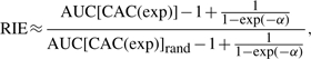
Although derived from different standpoints, additional metrics proposed in the literature are linear affine transforms of our metrics and can be written in the present notation. Specifically, Sheridan et al. (2001), Truchon and Bayly (2007) and Zhao et al. (2009) have, respectively, proposed to use the RIE, the BEDROC and the SLR metrics. The RIE metric corresponds to

(12)

where AUC[CAC(exp)]_rand is the area under the concentrated AC curve obtained by exponential transformation [CAC(exp)] of the random classifier. The BEDROC metric corresponds to

(13)

where AUC[CAC(exp)]_max and AUC[CAC(exp)]_min are, respectively, the area under the best and worst possible CAC(exp) curves. The SLR metric can be approximated as

(14)

where N is the total number of test candidates being scored and N₊ the number of positives. Thus RIE and BEDROC are affine transforms of AUC[CAC] and have the same statistical power as AUC[CAC]. SLR is an affine transform of AUC[pAC] and have the same statistical power as AUC[CAC]. Note that the approximation error in Equations (12) and (14) is negligible since it is less than the fluctuations introduced by the ambiguity in the definition of the AC curve and its area, depending on whether one uses the rectangular or trapezoidal rule, corresponding to whether consecutive points are connected by discrete jumps or linear interpolation. These fluctuations become also irrelevant on large datasets. Ignoring these fluctuations, which only subtly alter the computations, REI and BEDROC have a geometric interpretation depicted in Figure 3. The particular standpoints originally used to derive these other metrics did not lend themselves to deriving a more general magnification framework that can be extended, for instance, from AC to ROC curves, or to different magnification functions, or to derive corresponding visualizations. Furthermore, both the RIE and SLR metrics are larger than one and their ranges vary with the dataset to which they are applied, which is somewhat at odds with most other commonly used metrics for classification. The unifying framework presented here addresses all these issues.

Fig. 3.

The geometric relationship between the CAC(exp) curve and two early recognition metrics. Each letter, from A to F, corresponds to an area delimited by curves and the boundary of the plot. Both the RIE and BEDROC metrics can be expressed as ratios of particular areas of the plot.

Our data also suggests that the CROC(exp), the variant we propose for general use in early recognition, has better statistical power than other commonly used metrics (ROC, pROC, SLR, REI and BEDROC). It is tempting to perform more exhaustive benchmarks of statistical power on simulated datasets. However, the best strategy for simulating the appropriate data randomly is unclear. One strategy has been suggested by Truchon and Bayly (2007) and used by others. This strategy, however, assumes that the cumulative distribution of ranks is exactly the exp transform. This assumption is made without clear justification and could introduce some circularity and artificially bias tests of power toward metrics based on the exp transform. Although less exhaustive, we expect that direct comparison of metrics on real, rather than simulated, dataset will continue to provide unbiased insight into the utility of early recognition performance metrics.

Here, we have presented a general-principled approach for ‘putting a microscope’ on any portion of the ROC (or AC) curve, particularly the early part, to amplify events of interest and disambiguate the performance of various classifiers by measuring the relevant aspects of their performance. The magnification is mediated by a concave-down transformation f with a global magnification parameter α that allows one to smoothly control the level of magnification. Rational approaches for choosing the transformation and magnification factors have been proposed.

This magnification approach is sensitive to the rank of every positive candidate, and therefore should be preferred over all single threshold metrics. At the same time, the approach is sensitive to early recognition performance and can discriminate between predictors where standard methods fail, as seen in the drug discovery example used here. Unlike some of the previous visualizations and metrics (RIE, pROC and SLR), the CROC and CAC are both normalized to fit within the unit square and lead to an efficient visualization and measurement of early retrieval performance, with robust and tunable magnification. The overall approach has been demonstrated on a standard, publicly available, drug discovery benchmark dataset and a Python package that implements the CROC methodology is publicly available.

Funding: Laurel Wilkening Faculty Innovation award; an NIH Biomedical Informatics Training grant (LM-07443-01); NSF grants EIA- 0321390, CCF-0725370, and IIS-0513376 (to P.B.); IBM PhD Fellowship (to C.A.); Physician Scientist Training Program of the Washington University Pathology Department (to S.J.S.).

Conflict of Interest: none declared.

APPENDIX A

A.1 MAXIMIZING EARLY RETRIEVAL

An important question is whether a learning algorithm can be developed to emphasize early recognition, as opposed to classification or ranking over the entire data. A possible approach to address this issue is to try to optimize CROC behavior, rather than ROC behavior by, for instance, maximizing the AUC[CROC] rather than the AUC[ROC]. To this end, we propose an iterative algorithm where the training examples are reweighted after each training epoch giving, everything else being equal, higher weights to higher ranked examples. We describe several variations on this basic idea and explore them in the simulations. We assume that there are N training examples. All the examples are initialized uniformly, with a weight equal to 1/N. After each training epoch t, the weights are recomputed according to a polynomial or exponential decaying scheme of the form

(A1)

where w_r(t + 1) denotes the weight of the example with ranking r = r(t) after the first t epochs. The constant C is used to normalize the weights so that their sum remain constant.

A first variation on this idea is to multiply the weight update rule by the density of the scores that are in the neighborhood of the score of the example ranked r so that

(A2)

Here, g(r) represents the empirically measured or continuously smoothed density of the classifier scores around the score of the r-th ranked example. Intuitively, if this density is high, slightly improving the classification score of the corresponding example ought to have a larger effect than if the density is low. Other schemes not explored here could use differentially the density of positive and negative examples.

A second variation on this idea is to change the parameter γ during training, increasing it monotonically at each epoch, according to some schedule, linear or other. As in simulated annealing, the goal is to start with low values of γ to avoid getting stuck in early local minima.

In the corresponding series of experiments, for clarity we focus on the IRV exclusively, but in principle the same ideas can be applied to any learning method that allows for weighting the importance of the training instances. Table A1 shows the results for exponential weighting schemes, which greatly speed up the convergence of the algorithm, by a factor of 10 or so. Four to eight epochs of training with exponential weighting of the examples is sufficient to reach convergence. In contrast, the unweighted IRV requires 101 epochs. Although the final results obtained with exponential weighting are slightly inferior to those obtained without any weighting, the weighted IRV still outperforms the SVM and kNN algorithms. When a multiplicative factor associated with the density of the classifier scores around a given example is introduced into the weighting scheme, mixed results are observed.

Table A1.

Comparison of the AUC[CROC] (α = 80) of several weight update schemes for the IRV, after three training iterations and after convergence of the algorithm, together with the total number of iterations for convergence

	No weight	wr = e−r/N
		Regular	×g(r)	Regular	×g(r)
AUC[CROC]	0.368	0.383	0.364	0.374	0.383
After three iterations
AUC[CROC]	0.404	0.388	0.381	0.383	0.385
After convergence
Iterations	101	8	4	4	5

Results are 10-fold cross-validated on the HIV dataset. Best performances are in bold and second-best performances are in italics.

As shown in Table A2, the 1/r power-law weighting scheme performs the best in this case, converging three times faster than the unweighted IRV, and reaching a set of weights that gives the same level of performance, in terms of early enrichment or AUC[CROC], as in the unweighted case. Convergence takes 42 epochs, and only 33 epochs if multiplied by the density g(r), as opposed to 101 epochs in the unweighted case. Although after convergence the AUC[ROC] in the weighted and unweighted cases seem identical (0.396), the compounds are ranked similarly but not identically. This is why the AUC[CROC] are slightly different for α = 7 and, with more decimal precision, the AUC[CROC] with α = 80 can be differentiated. In any case, on this dataset, we see that for the power (1/r) weighting scheme, multiplication by the density g(r) slightly improves both the speed of convergence and the quality of the final classifiers. In summary, this learning scheme can sometimes slightly improve the performance of a classifier, while quite often dramatically speeding up the time it takes to train a model by gradient descent. In our study, this speed-up can be close to 2-fold.

Table A2.

Comparison of the AUC[CROC] (α = 7 and α = 80) of the regular IRV and the IRV with weights updated by w_r = 1/r multiplied or not by the output density g(r), presented after one and three iterations and after convergence of the algorithm

	AUC[CROC] (α = 7)			AUC[CROC] (α = 80)
	wr = 1	wr = 1/r	wr = g(r)/r	wr = 1	wr = 1/r	wr = g(r)/r
After one iteration	0.569	0.598	0.611	0.348	0.365	0.366
After three iterations	0.641	0.646	0.652	0.368	0.380	0.386
After convergence	0.660	0.660	0.661	0.404	0.403	0.404

The IRV converges after 101 iterations if the weights are not updated, 42 if they are updated by w_r = 1/r and 33 if they are updated by w_r = g(r)/r. Results are 10-fold cross-validated on the HIV dataset. Best performances are in bold and second-best performances are in italics.

REFERENCES

- Azencott C, et al. One- to four-dimensional kernels for small molecules and predictive regression of physical, chemical, and biological properties. J. Chem. Inf. Model. 2007;47:965–974. doi: 10.1021/ci600397p. [DOI] [PubMed] [Google Scholar]
- Baldi P, et al. Assessing the accuracy of prediction algorithms for classification: an overview. Bioinformatics. 2000;16:412–424. doi: 10.1093/bioinformatics/16.5.412. [DOI] [PubMed] [Google Scholar]
- Clark RD, Webster-Clark DJ. Managing bias in ROC curves. J. Comput. Aided Mol. Des. 2008;22:141–146. doi: 10.1007/s10822-008-9181-z. [DOI] [PubMed] [Google Scholar]
- Hassan M, et al. Cheminformatics analysis and learning in a data pipelining environment. Mol. Divers. 2006;10:283–299. doi: 10.1007/s11030-006-9041-5. [DOI] [PubMed] [Google Scholar]
- Hert J, et al. Comparison of fingerprint-based methods for virtual screening using multiple bioactive reference structures. J. Chem. Inf. Model. 2004;44:1177–1185. doi: 10.1021/ci034231b. [DOI] [PubMed] [Google Scholar]
- Hert J, et al. Enhancing the effectiveness of similarity-based virtual screening using nearest-neighbor information. J. Med. Chem. 2005;48:7049–54. doi: 10.1021/jm050316n. [DOI] [PubMed] [Google Scholar]
- Holliday JD, et al. Grouping of coefficients for the calculation of inter-molecular similarity and dissimilarity using 2D fragment bit-strings. Comb. Chem. High Throughput Screen. 2002;5:155–66. doi: 10.2174/1386207024607338. [DOI] [PubMed] [Google Scholar]
- Leach AR, Gillet VJ. An Introduction to Chemoinformatics. Dordrecht, Netherlands: Springer; 2005. [Google Scholar]
- Mahé P, et al. The pharmacophore kernel for virtual screening with support vector machines. J. Chem. Inf. Model. 2006;46:2003–2014. doi: 10.1021/ci060138m. [DOI] [PubMed] [Google Scholar]
- Seifert M.HJ. Assessing the discriminatory power of scoring functions for virtual screening. J. Chem. Inf. Model. 2006;46:1456–1465. doi: 10.1021/ci060027n. [DOI] [PubMed] [Google Scholar]
- Sheridan R, et al. Protocols for bridging the peptide to nonpeptide gap in topological similarity searches. J. Chem. Inf. Comput. Sci. 2001;41:1395–1406. doi: 10.1021/ci0100144. [DOI] [PubMed] [Google Scholar]
- Swamidass S, et al. The Influence Relevance Voter: An Accurate And Interpretable Virtual High Throughput Screening Method. J. Chem. Inf. Model. 2009;49:756. doi: 10.1021/ci8004379. [DOI] [PMC free article] [PubMed] [Google Scholar]
- Swamidass SJ, Baldi P. Bounds and algorithms for exact searches of chemical fingerprints in linear and sub-linear time. J. Chem. Inf. Model. 2007;47:302–317. doi: 10.1021/ci600358f. [DOI] [PMC free article] [PubMed] [Google Scholar]
- Swamidass SJ, et al. Kernels for small molecules and the predicition of mutagenicity, toxicity, and anti-cancer activity. Bioinformatics. 2005a;21(Suppl. 1):359. doi: 10.1093/bioinformatics/bti1055. [DOI] [PubMed] [Google Scholar]
- Swamidass SJ, et al. Kernels for small molecules and the prediction of mutagenicity, toxicity, and anti-cancer activity. Bioinformatics. 2005b;21(Suppl. 1):i359–368. doi: 10.1093/bioinformatics/bti1055. [DOI] [PubMed] [Google Scholar]
- Truchon JF, Bayly CI. Evaluating virtual screening methods: Good and bad metrics for the “early recognition” problem. J. Chem. Inf. Model. 2007;47:488–508. doi: 10.1021/ci600426e. [DOI] [PubMed] [Google Scholar]
- Zhao W, et al. A statistical framework to evaluate virtual screening. BMC bioinformatics. 2009;10:225. doi: 10.1186/1471-2105-10-225. [DOI] [PMC free article] [PubMed] [Google Scholar]