Epigenetic Contribution to Covariance Between Relatives

Abstract

Recent research has pointed to the ubiquity and abundance of between-generation epigenetic inheritance. This research has implications for assessing disease risk and the responses to ecological stresses and also for understanding evolutionary dynamics. An important step toward a general evaluation of these implications is the identification and estimation of the amount of heritable, epigenetic variation in populations. While methods for modeling the phenotypic heritable variance contributed by culture have already been developed, there are no comparable methods for nonbehavioral epigenetic inheritance systems. By introducing a model that takes epigenetic transmissibility (the probability of transmission of ancestral phenotypes) and environmental induction into account, we provide novel expressions for covariances between relatives. We have combined a classical quantitative genetics approach with information about the number of opportunities for epigenetic reset between generations and assumptions about environmental induction to estimate the heritable epigenetic variance and epigenetic transmissibility for both asexual and sexual populations. This assists us in the identification of phenotypes and populations in which epigenetic transmission occurs and enables a preliminary quantification of their transmissibility, which could then be followed by genomewide association and QTL studies.

EPIGENETIC inheritance involves the transgenerational transmission of phenotypic variation by means other than the transmission of DNA sequence variations. Cellular epigenetic inheritance, where transmission of phenotypic variation involves passing through a single-cell stage (the gametic stage in sexually reproducing multicellualr organisms), is now recognized to be an important and ubiquitous phenomenon and the mechanisms underlying it are becoming elucidated (Jablonka and Lamb 2005; Allis et al. 2007; Jablonka and Raz 2009). Epigenetic inheritance occurs between generations of asexually and sexually reproducing organisms, directly affecting the hereditary structure of populations and providing a potential mechanism for their evolution (Jablonka and Lamb 1995, 2005; Bonduriansky and Day 2009; Jablonka and Raz 2009; Verhoeven et al. 2009). It is therefore necessary to develop tools to study its prevalence and estimate its contribution to the heritable variance in the population (Bossdorf et al. 2008; Johannes et al. 2008, 2009; Richards 2008; Reinders et al. 2009; Teixeira et al. 2009).

Unlike epigenetic inheritance, the inheritance of cultural practices in human populations has received a great deal of theoretical attention. Models of cultural inheritance and of interacting cultural and genetic effects have been suggested (Cavalli-Sforza and Feldman 1973; Rao et al. 1976; Cloninger et al. 1978; Boyd and Richerson 1985; Richerson and Boyd 2005). These models study the effects of cultural transmission and analyze the way in which it affects the distribution of cultural practices in the population. Other aspects of transgenerational effects are revealed through the study of maternal or indirect genetic effects (Kirkpatrick and Lande 1989; Wolf et al. 1998) and transgenerational genetic and epistatic effects within the context of the “missing heritability” problem (Nadeau 2009).

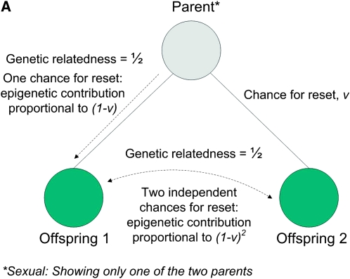
The simple models described in this article focus on the transmissibility of epigenetic variations rather than on the magnitude of the phenotypic expression. In that respect, epigenetic inheritance is generally simpler to model than cultural inheritance since it commonly involves only vertical transmission (from parent to offspring). Crucially, during early development, as well as during gametogenesis and meiosis, some of the parental epigenetic information is restructured and reset. It is therefore necessary to explicitly include in models of epigenetic inheritance the number of developmental-reset generations. The number of developmental-reset generations between relatives may differ even when genetic relatedness is the same: for example, the relatedness between parent and offspring is 0.5 and so is the relatedness between sibs (on average), but the number of developmental-reset generations is one and two, respectively. These considerations are also valid for asexual organisms, if it is assumed that some form of reset occurs during the cell cycle between divisions. In this case we can test the models and measure the contribution of epigenetic inheritance in well-defined experimental conditions, in pure lines.

To estimate the amount of heritable epigenetic variation, we need to define several concepts: heritable epigenetic variability, the reset coefficient, and its complement, the epigenetic transmission coefficient. Heritable epigenetic variability refers to phenotypic variability that is determined by epigenetic states that are environmentally induced and also possibly inherited from previous generations. The heritable variations on which epigenetic heritability depends can arise spontaneously (as a particular type of developmental noise), or they can be environmentally induced. Once present, these variations can be vertically transmitted. For example, variations in methylation patterns between individuals may contribute to phenotypic variability even if these individuals are all genotypically identical. Such variations have been found in several systems (Jablonka and Raz 2009). When the methylation marks are transmitted between generations, this will contribute to inherited epigenetic variability. The reset coefficient (v) refers to the probability of changing the epigenetic state during gametogenesis and/or early development, so that the new generation can respond to the present environmental conditions with no memory of past environments. The complement of this reset coefficient, 1 − v, is the coefficient of epigenetic transmissibility: the probability of transmitting the epigenetic state to the next generation, without reset. The epigenetic transmission coefficient should be taken as an abstraction that encapsulates all the potentialities of epigenetic inheritance related to the target phenotype, over a single generation. While we express the coefficient as a probability, it may also be interpreted as ratio coefficient, representing the portion of the epigenetic value that is transmitted to the next generation. In terms of the model these two interpretations are equivalent. The model also makes the simplifying assumption that the reset coefficient is a constant of the population, although in reality it might assume some distribution.

We determine the above terms for both asexually and sexually reproducing organisms within a quantitative genetics framework. We suggest that terms including the effects of reset and epigenetic transmissibility be included in the classical model of phenotypic variance, showing how these terms can be calculated from the covariances between relatives. Morphological and physiological phenotypes can be assessed in this way, and if the results point to an epigenetic component of inheritance, the underlying epigenomic bias can be investigated by employing QTL and association studies (Johannes et al. 2008; Reinders et al. 2009). A recent study using these methods provides evidence that epigenetic variation can contribute significantly to the heritability of complex traits (∼30% heritability), introducing transgenerational stability of epialleles into quantitative genetic analysis (Johannes et al. 2009). Our model, which entails direct measurements of phenotypic covariation, should provide only preliminary and rough approximations of epigenetic transmissibility for target traits and populations.

MODELS AND MEASURES OF EPIGENETIC VARIANCE, RESET, AND TRANSMISSIBILITY

We consider a continuous trait with genetic, epigenetic, and environmental variability. First we develop the model for the case of asexual reproduction; sexual outbreeding populations follow. The phenotypic value of an individual (P) is given by the sum of the genetic value (G), the heritable epigenetic contribution (C), and the environmental deviation (E). Instead of the standard quantitative genetics model P = G + E we use P = G + C + E as our basic model, assuming independence and additivity, for simplicity. The two models are effectively equivalent, since in the classical equation E includes all nongenetic effects, of which our C may be one component. Alternatively, C may be included in G, since the variance attributable to heritable effects is sometimes assumed to be purely of genetic origin. The epigenetic value of an offspring depends on whether its epigenetic state was reset. If reset, the epigenetic contribution is determined by the inducing environment, I_t. Offspring that are not reset inherit the epigenetic state, C, of their parents. An offspring resets its epigenetic state with probability v (the reset coefficient) and inherits the parent's epigenetic state with probability 1 − v (the epigenetic transmissibility coefficient).

The inducing environment, I_t, can be an exposure to an environmental signal or stress (e.g., a heat shock, an exposure to a chemical such as the demethylating agent 5-azacytidine, or exposure to an androgen suppressor such a vinclozolin), which elicits a developmental reaction. Alternatively, it can be a mutation that has developmental effects that persist after the mutation itself has been segregated away. An example is the effect of ddm1 mutation in Arabidopsis, which leads to wide-ranging demethylation, with some demethylated patterns persisting many generations after the original mutation has been segregated away and the normal wild-type allele has been introduced (Reinders et al. 2009; Teixeira et al. 2009). Another type of genomic shock leading to heritable epigenetic responses is hybridization followed by polyploidization (allopolyploidy). In these cases, notably in the case of Spartina hybrids, the newly formed allopolyploids acquire genomewide epigenetic variations, some of which are heritable for many generations (Salmon et al. 2005). When the inducing environment involves an environmental change, random or periodic changes in the inducing environment maintain epigenetic variability in the population and can render a selective advantage to epigenetic inheritance compared to noninducible genetic or nonheritable plastic strategies (Jablonka et al. 1995; Lachmann and Jablonka 1996; Ginsburg and Jablonka 2009).

The epigenetic contribution of a reset offspring in year t is a random value taken from a distribution determined by the current inducing environment I_t; it is independent of the parental epigenetic state, C. Due to the temporal variation and epigenetic transmissibility, the population mean of the epigenetic contribution changes in time as an autoregressive process, . In contrast to the inducing environment, the microenvironmental factors that determine the environmental deviation (E) vary among individuals within a generation, but on average do not change in time, such that the expected value of E is zero. We assume that G, C, and E are statistically independent such that

(1)

Two questions arise when the epigenetic term is introduced: (1) Can we distinguish, by quantitative genetic analysis, between heritable epigenetic and genetic inheritance? and (2) How can we estimate the epigenetic transmissibility coefficient, (1 − v)?

Both questions can be addressed by comparing covariances between relatives. There are three unknowns to be estimated, the genetic variance, V_G, the heritable epigenetic variance V_C, and the epigenetic transmissibility coefficient (1 − v), since these are the only parameters that contribute to the covariances. Therefore we need to compare three covariances between relatives that contain the genetic and epigenetic variance components in different proportions. The simplest way is to measure the covariance between parents and offspring, between sibs, and between uncles and nephews. We employ these anthropomorphic relational terms to maintain standard parlance within quantitative genetics.

We differentiate between two major types of asexual reproduction: (i) asymmetric transmission, where a parent organism is not identical to its offspring following cell division (this is the case following reproduction by budding, with the parent organism able to bud off several offspring over time), and (ii) symmetrical cell division, where the parent cell is also the offspring cell, as occurs in many unicellular organisms and in cell lineages. In epigenetic terms, symmetrical reproduction leads to common reset potential for both daughter cells (either both reset or neither of them do), but the inducing random epigenetic contributions they obtain are independent. In this case, single cells have to be followed over generations for the family relations to be established. We assume that asexual asymmetric reproduction involves a developmental process of the offspring that the parent need not go through, and it is during this process that developmental reset may occur (there may be a degree of reset in the parent too, in some cases).

We begin by describing the specifics of the mathematical model as it pertains to asymmetric asexual reproduction, follow up with the unicellular symmetrical asexual case, and end with the sexual reproduction case.

Asexual asymmetric reproduction:

Consider a parent with phenotype P = G + C + E undergoing asexual reproduction. The mean phenotype of its offspring is

(2)

Note that there is no microenvironmental term in (2), since we employed the mean offspring value, and the mean microenvironmental deviation is defined to be zero across the population.

The parent–offspring covariance

(3)

follows directly from the assumption that G, E, C, and are mutually independent and from the fact that the covariance of any individual with the mean value of a number of relatives is equal to its covariance with any one of those relatives (Falconer and Mackay 1996). The covariance of sibs equals the variance of the true means of sib groups, which is

(4)

assuming does not covary between siblings.

Note that the heritable epigenetic variance contributes less to the covariance between sibs than to the covariance between parents and offspring. Under asexual reproduction, purely genetic variability results in equal covariances between relatives. A significant difference between COV_OP and COV_SIB therefore may suggest heritable epigenetic variability.

The covariance between uncles and nephews is (see appendix)

(5)

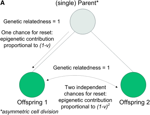
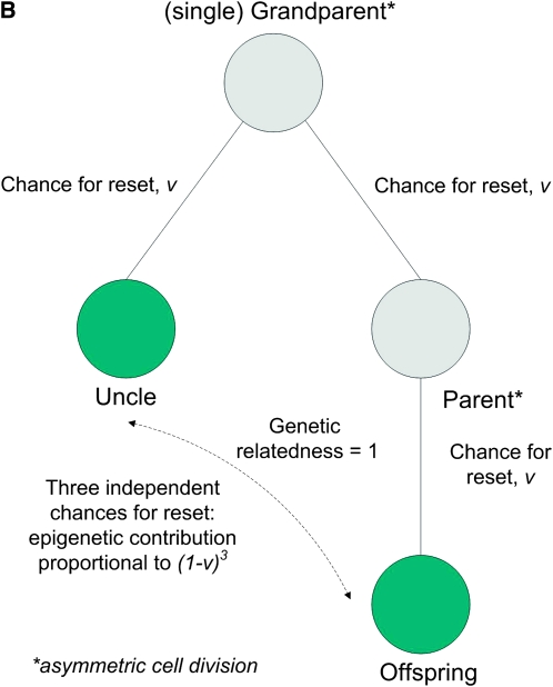
Figure 1, A and B, depicts how the epigenetic contribution to the similarities between relatives depends on the opportunities for epigenetic resets, in asexual species, for parent–offspring, between-sibling, and uncle–nephew relations.

Figure 1.—

(A) Parent–offspring and full sibling similarities in asymmetric asexual reproduction: the genetic relatedness is the same in both cases, while the epigenetic contribution differs. (B) Uncle–nephew similarity in asymmetric asexual reproduction: the epigenetic contribution is proportional to (1 − v)³.

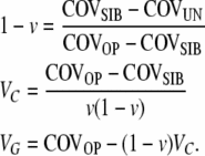
From Equations 3–5 one can calculate the variance components and the epigenetic transmissibility coefficient as

(6)

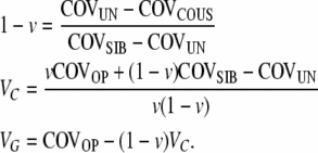
If the covariance estimates COV_SIB and COV_OP are approximately equal, then it can be shown from the derivation of (6) that either V_C is near zero (i.e., a single value to the epigenetic effect) or the reset coefficient v is close to its extreme values of one or zero. We would not be able to distinguish between these three distinct possibilities, all of which are theoretically viable. This introduces a singularity point inherent in our model, which we acknowledge, and in such a case the model is inapplicable for the target phenotype and population. The same cautionary note applies to (8) below for COV_SIB = COV_UN and to (9) for COV_OP = 2 COV_HS. Furthermore, v = 0 would mean that epigenetic effects become indistinguishable from genetic effects; similarly, v = 1 means that epigenetic effects are always reset and therefore indistinguishable from environmental effects.

Note that we could extract estimates of heritability from our model, since it also generates V_G. Checking such estimates with reference to various traits against known heritability values should provide a further indication as to the soundness of our model. Moreover, V_G will be effectively zero if the population has a single recent ancestor (not withstanding the possible mitotic mutations over generations). In that case we should expect COV_OP to be equal to (1 − v)V_C, and any deviation from this equality may indicate a flaw in the model.

As a consequence of the changes in the inducing environment, I_t, across generations and consequently in the distribution of , the epigenetic variance may change in time. Therefore the ancestors of the measured relatives, i.e., the parent in Equation 3, the parent of the sibs in Equation 4, and the parent of the uncle (grandparent of the nephew) in Equation 5, must belong to the same generation, and V_C is the variance of the epigenetic contribution in this ancestral generation.

Asexual symmetric reproduction:

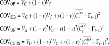
Here the focus is on a population of unicellular organisms or cell lineages. This case is naturally limited in lending itself to large-scale statistical quantitative analysis, as meticulous tracing of cell lineages across generations is required for producing the covariances. Since the offspring resets are not independent, we require examining also the covariance of cousins, labeled COV_COUS, when solving for the three unknowns. Additionally, the possibility of a fluctuating inducing environment across generations introduces an extra term in three of the covariances (see appendix), such that

(7)

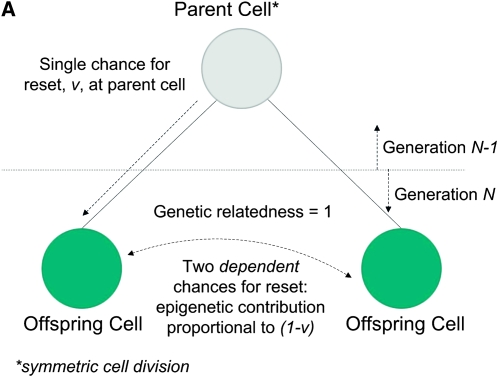
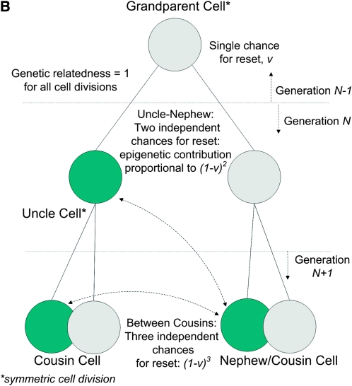
Figure 2, A and B, depicts how the epigenetic contribution to the similarities between relatives depends on the opportunities for epigenetic resets across single and multiple generations of offspring cells in an asexual species with symmetric reproduction.

Figure 2.—

(A) Parent–offspring and between-sibling similarities in symmetrical asexual reproduction: single chance for reset for both offspring. (B) Uncle–nephew and between-cousin similarities in symmetrical asexual reproduction: the parent cell and the uncle cell share a single chance for reset.

We then arrive at the solution for our three unknowns,

(8)

Sexual reproduction:

We assume that the parents contribute equally to the epigenetic contribution of their nonreset offspring. This assumption is valid for chromosomally transmitted epigenetic information, such as methylation patterns, histone modifications, nonhistone DNA binding proteins, and nuclear RNAs. When heritable epigenetic variations are cytoplasmic or cortical, the mother alone transmits the epigenetic variation, and when only the female lineage is considered, the variations produced by these epigenetic inheritance systems can be analyzed in the same way as variations transmitted by asexual, asymmetrically reproducing organisms. Here we consider chromosomally transmissible epigenetic variations as well as variations mediated through the RNAi system and assume equal contribution by both parents. It is likely that during sexual reproduction, the reset mechanism is more comprehensive than in asexual reproduction. However, as in the asymmetric asexual scenario, the offspring here reset independently.

The heritable epigenetic component creates several discrepancies from the standard quantitative genetic relations. Due to the larger fraction of epigenetic variance contributed to the parent–offspring covariance, COV_OP is more than twice the covariance between half sibs (COV_OP > 2 COV_HS); however, this difference could also be explained by the effect of additive–additive interaction. A more conclusive comparison is between the uncle–nephew and the half-sib covariance. Uncles and nephews as well as half sibs are second-degree relatives with a single common ancestor, and therefore their covariance contains exactly the same genetic variance components. However, the epigenetic variance contributes more to the covariance between half sibs (COV_HS > COV_UN). Detecting a greater covariance between half sibs therefore would provide good evidence for epigenetic inheritance.

Comparison of the full-sib and parent–offspring covariances might also reveal the presence of heritable epigenetic variation. The epigenetic contribution increases COV_OP more than COV_FS while the additive genetic contribution is the same; thus COV_FS < COV_OP would be expected. However, dominance and maternal effects can increase COV_FS considerably and hence somewhat mask the effect of heritable epigenetic variation. The presence and magnitude of the obscuring dominance and maternal effects can be assessed by sib analysis (Falconer and Mackay 1996, p. 166). Sib analysis makes use of the fact that without dominance and maternal effects the full-sib covariance should equal twice the half-sib covariance. This remains true even in the presence of heritable epigenetic variation, so sib analysis can be applied to measure dominance and maternal effects without any distortion due to the heritable epigenetic effects. Removing the dominance and maternal effects from the full-sib covariance facilitates the detection of heritable epigenetic variability by comparison of the full-sib covariance with the parent–offspring covariance. For simplicity, we assume no dominance or epistatic effects [for instance, one-eighth of the additive–additive variance contributes to COV_OP − 2 COV_HS in (9)] and suggest using paternal half siblings where maternal effects are absent.

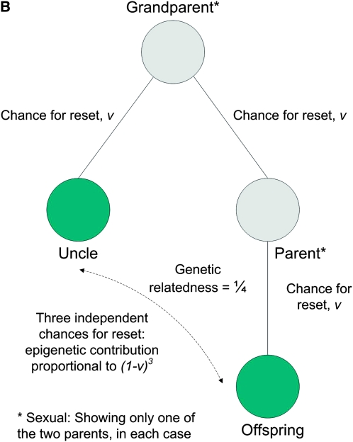
Figure 3, A and B, depicts how the epigenetic contribution to the similarities between relatives depends on the opportunities for epigenetic resets in sexual species.

Figure 3.—

(A) Parent–offspring and full sibling similarities in sexual reproduction: two independent chances for reset between offspring, while their genetic relatedness is . (B) Uncle–nephew similarity in sexual reproduction: three independent chances for reset between uncle and nephew, while the genetic relatedness is .

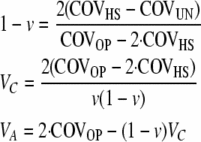
The variance components and the epigenetic transmissibility coefficient can be estimated from the measured covariances as

(9)

(see appendix), where the uncle and the parent of the nephew are full sibs, and, as before, the parent in COV_OP, the parent of the half sibs, and the parent of the uncle (grandparent of the nephew) belong to the same generation.

DISCUSSION AND CONCLUSION

Transgenerational, ecologically or developmentally induced phenotypic variations have been studied mainly in the context of maternal effects and have been treated as temporally extended developmental effects (Wolf et al. 1998). The study of cultural transmission, on the other hand, was confined to studying the complex system of transmission of cultural practices (Boyd and Richerson 1985; Feldman and Laland 1996). As a consequence, quantitative studies of the transmission rather than the expression of heritable epigenetic variations have only in recent years begun to surface, although molecular studies have been around for some time showing that epigenetic marks such as DNA methylation patterns, protein marks, and RNA-mediated silencing can be inherited (reviewed in Jablonka and Raz 2009).

In the absence of detailed molecular studies, it is often very difficult to detect epigenetic inheritance, since deviations from classical Mendelian ratios can be always explained by assuming interactions with modifier genes. In asexually reproducing, multicellular organisms, rapid and heritable phenotypic switches are usually explained within the framework of somatic mutations and somatic selection or various types of phase variations.

It is instructive to suggest a formulation of the extent of heritable epigenetic variation. The epigenetic heritability, denoted here by γ², is the proportion of the total phenotypic variance V_P attributable to the potentially heritable epigenetic variance V_C,

(10)

Contrary to the standard notion of heritability where V_G is always heritable variance, the epigenetic heritability, by definition, does not directly depend on the epigenetic transmissibility coefficient, (1 − v), but only on V_C. However, the extent to which epigenetic heritability contributes to the measurable regression or correlation coefficients does depend on the epigenetic transmissibility of the epigenetic inheritance system. For example, in parent–offspring regression, a fraction (1 − v) of the epigenetic heritability always increases the regression slope:

(11)

In general, the epigenetic contribution to the regression of two related individuals would be , where n is the number of independent opportunities for epigenetic reset in the lines of descent connecting the relatives.

The inducing environment, I_t, may determine the epigenetic contribution after reset in a deterministic fashion, such as under extreme stress conditions, in which case the distribution of becomes a delta-peak. In a situation where I_t ceases to vary at generation k, the reset individuals always acquire a new epigenetic contribution from the same distribution , so the distribution of C will converge on the distribution of C^(r) and . In the extreme case when I_t both is time independent and unequivocally determines the induced epigenetic contribution, the distribution of C converges to a delta-peak; no heritable epigenetic variation is present.

In the model presented in this article we assumed that v, the reset coefficient, is independent of the number of generations that the lineage spent in a particular environment prior to the switch to a new inducing environment. However, it is possible that the number of generations a lineage spends in a given environment may alter the probability of a phenotypic switch. Transfer experiments, in which the number of generations spent in each environment is varied, and v and 1 − v are measured for each case, may uncover such phenomena. Other factors that may affect the stability of epigenetic inheritance are the number of generations a chromosome is transmitted through only one sex (e.g., a male) and the number of generations that chromosomes are continuously transmitted though an aged parent (Jablonka and Lamb 2005).

What values of the epigenetic transmissibility coefficient and epigenetic heritability should alert us to the possibility that part of the observed variance is due to epigenetic variation? Ideally, we want to have threshold values for each phenotype under consideration, so that only values obtained through the model that lie above it would provide sufficient confidence for further molecular inspection (see the appendix for a suggestion for employing a workable probabilistic threshold). In terms of the epigenetic transmissibility coefficient, it is reasonable to treat any value above zero as indicative of possible heritable effects, even if only for a very small number of generations and individuals.

The detection and measurement of epigenetic heritability may suggest new testable interpretations of a number of observations. For example, experiments measuring heritability in inbred lines showed that heritability increases fairly rapidly in inbred sublines of different organisms (Grewal 1962; Hoi-Sen 1972; Lande 1976). These results were interpreted to mean that many genes contribute to a character and that the rate of mutation of these genes is high. The mutation rates calculated from the data with the assumption that mutations alone contribute to heritability were two to three orders of magnitude higher than the traditionally estimated rate of classical mutation (Hoi-Sen 1972). But the high heritability appearing after relatively few generations of subline divergence can be reinterpreted as being partly due to heritable epigenetic variability, especially in view of more recent molecular studies that show that epigenetic inheritance occurs in pure lines (Johannes et al. 2008, 2009; Reinders et al. 2009). When a subline of a highly inbred line is started from a pair of individuals, epigenetic variations (epimutations) as well as mutations will accumulate as the subline diverges. As the rate of epimutation by epigenetic reset is often much higher than that of mutation, heritable epigenetic variability will grow more rapidly than genetic variability. The fraction of epigenetic variability should be relatively high, especially during the first generations of a subline divergence, when it is the sole contributor to heritable variance. Since the epigenetic heritability can be measured from the covariances between relatives within the line, this hypothesis can be tested.

The hypothesis that there is a heritable epigenetic component of phenotypic variance has the implication that selection can be effective in genetically pure lines. Some observations indicate that this is indeed the case (Brun 1965; Ruvinsky et al. 1983a,b; see Johannes et al. 2009 for a precise estimate based on QTL analysis). The response to selection in one generation is determined by the midparent–offspring regression coefficient, b=h²+(1−v)γ². Since pure lines may acquire epigenetic variability relatively quickly, and this variability contributes to the regression, the response to selection enabled by the epigenetic heritability can be readily measurable. The realized heritability in a genetically pure line will then estimate (1−v)γ². Note that once selection is relaxed, all effects achieved by previous selection on the epigenetic variability are sooner or later lost (at a rate depending on epigenetic transmissibility), unless the phenotype is by then stabilized by genetic assimilation (Ruden et al. 2005, 2008; Shorter and Lindquist 2005).

We have shown that epigenetic heritability can be measured for both asexually and sexually reproducing organisms. A promising system in which to measure epigenetic heritability is in inbred lines of plants, since plants seem to have particularly sophisticated cellular mechanisms of adaptation, and several cases of epigenetic inheritance based on chromatin marks have been reported in plants (Jablonka and Raz 2009). The phenotypic effects of altering environmental conditions have been studied in plants, and data on the frequency of phenotypic change are known for some cases (Bossdorf et al. 2008; Johannes et al. 2008, 2009; Richards 2008; Reinders et al. 2009; Whittle et al. 2009).

The novelty of our approach lies in the attempt to quantify a measure of epigenetic variability using classical notions of familial phenotypic covariances. Other approaches have looked at the actual epigenetic variability, with the goal of producing a quantifiable measure of the variability with respect to a certain locus or a related group of loci. One such research looked at epigenetic variability in the germline, formulating an average methylation-intensity vector for each locus/individual, by looking at the sum of the methylated cytosines for each different cytosine position. The degree of epigenetic dissimilarity was then defined via the Euclidean distance between the vectors of the two individuals (Flanagan et al. 2006).

A complementary approach to that presented here is proposed in Slatkin (2009). The model assumes that disease risk is affected by various diallelic genetic loci and epigenetic sites and takes allele frequencies and gain and loss rates of inherited epigenetic marks as input parameters. The mathematical iterative process of a two-state Markov chain is then utilized to simulate the state of the contributing loci after a number of generations. A central perspective that we believe is common to Slatkin's approach and ours is precisely this introduction of parameters for the quantitative effects of an inducing environment and reset coefficient and the realization that genetic and epigenetic factors contribute differently to familial similarities (recurrence risk, in Slatkin's case). However, our approach is distinct in that we employ and extend the standard quantitative genetic approach and utilize familial correlations in observed phenotypes as inputs to our model; it does not require prior estimations of gain and loss rates of inherited epigenetic marks or their frequency.

Studies focusing on the timing of changing the environment and applying an inducer can shed light on the sensitive periods of development, during which changed conditions can have long-term heritable effects. It has been shown that developmental timing is crucial for changed conditions to have long-term effects: for example, administering an androgen suppressor to a pregnant rat leads to heritable epigenetic effects only if the drug is administered during a sensitive period between days 8 and 15 of pregnancy (Anway et al. 2005).

Environmental insults, such as pollution, cause human (and nonhuman) diseases that may carry over for a number of generations (Jablonka 2004; Gilbert and Epel 2009). For instance, early paternal smoking was associated with greater body mass index at 9 years of age in sons (Pembrey et al. 2006). Such carry-over effects may be uncovered by careful search for transgenerational effects. The ability to detect and quantify a preliminary rough measure of transgenerational, environmentally induced diseases could become part of epidemiological studies.

The model presented here provides an initial estimate of epigenetic transmissibility that can be the basis for further molecular studies. We are well aware that a complete analysis of the developmental, and possibly evolutionary, effects of epigenetic inheritance has to include both transmissibility and expressivity and that QTL methodology is indispensable. However, a preliminary ability to empirically detect and quantify a rough measure of transgenerational epigenetic effects can give epidemiologically important information and assist in narrowing and directing the search domain for molecular epigenetic sequencing.

APPENDIX: DERIVATION OF FAMILIAL COVARIANCES

Asexual asymmetric reproduction:

For derivation of COV_UN consider an asexual parent (P) with two offspring (X and U) and an offspring of X denoted by N. U and N are uncle and nephew. The uncle was born in generation t − 1 and the nephew in generation t. Given the genotypic value, G_P, and the epigenetic contribution, C_P, of the common ancestor, the expected phenotypic value of the uncle is

(A1)

The nephew inherits the epigenetic contribution C_P only if neither it nor its parent resets the epigenetic state. If the nephew is not reset but its parent is reset, then it inherits ; if the nephew resets, then it takes a random value . Hence the expected phenotypic value of the nephew is given by

(A2)

From Equations A1 and A2 the uncle–nephew covariance is

(A3)

Asexual symmetric reproduction:

This case is complicated by the fact that due to simultaneous reset, a fluctuating inducing environment affects some of the familial covariances. The simultaneous reset of offspring does not affect the covariance between the parent and one of its offspring; hence

(A4)

just as in case of asexual asymmetric reproduction (see Equation 3 of the main text). To obtain the covariance between sibs, we must use conditional expectations and covariances. Within one family (with the parent having phenotype P = G + C + E), the conditional offspring mean is

(A5)

so that we get , [since we assumed that does not covary between siblings]. By the law of total covariance, the unconditional covariance equals the mean of conditional covariances,

plus the covariance of conditional means across the population. The population mean of the nonreset offspring is , whereas the mean of reset offspring is . Define X to be the conditional mean of the first offspring in a family and Y the conditional mean of the second offspring in a family. Their bivariate distribution is

The covariance of conditional means across the population is therefore , which readily simplifies to . Putting all terms together, the unconditional covariance between sibs is given by

(A6)

Note that if the inducing environment becomes constant across generations, then the autoregressive process converges to so that the last term of Equation A6 vanishes. It can be shown that unlike the covariance, the correlation of sibs increases with a large fluctuation in the mean of the inducing environment, but decreases with an increase in the variance of the inducing environment. A fluctuating inducing environment affects COV_SIB only in the symmetric case, since in the asymmetric case the bivariate distribution of siblings is such that the covariance of conditional means is always zero:

The covariance of conditional means is therefore

and similarly it is zero for the uncle–nephew covariance (asexual asymmetric case).

For the calculation of uncle–nephew and cousin covariances we express the conditional expectations of the uncle U and of the nephew N,

and

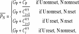where G_P is the genetic value and C_P the epigenetic contribution of the parent of the uncle. In accordance with the respective probabilities for reset, the mean of conditional covariances is

To obtain the unconditional covariance, we need to add the covariance of conditional means. If X is the conditional mean of the uncle and Y is that of the nephew, we have the bivariate probability,

The covariance of conditional means comes out to be . For the unconditional covariance between uncle and nephew we get

(A7)

For the between-cousin covariance, we first calculate the mean of conditional covariances,

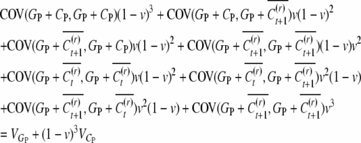and then add the covariance of conditional means. We denote X as one cousin and Y as the other cousin (where U is the father of the first cousin) and express their bivariate probability:

The covariance of conditional means comes out to be . So we have

(A8)

From (A4), (A6), (A7), and (A8) we solve for our three unknowns as expressed in (8), where the unknown term cancels out.

Sexual reproduction:

Here A denotes the breeding value so that V_A is the additive genetic variance; the mean breeding value is scaled to zero. With paternal phenotype P = A + C + E the offspring mean phenotype under random mating for paternal half siblings is

The offspring–parent and half sibling covariances are

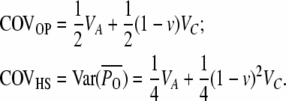(A9)

For the derivation of uncle–nephew covariance (the parent of the uncle should come from the same generation as the parents above), let M and F denote a mother and a father with two offspring, X and U, and an offspring of X denoted by N; U and N are uncle and nephew as before (the other parent of the nephew is an individual taken randomly from the population). The expected phenotypic values of the uncle and his sib X are the same,

(A10)

If the nephew did not reset his epigenetic state, then he inherits half the epigenetic contribution of X plus half the epigenetic contribution of a randomly chosen individual in generation t − 1. Therefore the nephew's expected phenotypic value is

(A11)

From Equations A10 and A11 the uncle–nephew covariance is calculated as

(A12)

where V_A = Var(A_M) = Var(A_F) and V_C = Var(C_M) = Var(C_F).

Identifying classes of individuals with large epigenetic contributions:

The objective is to find an expression for the probability that, for a given phenotypic deviation, P, |C| is greater than a certain threshold K, i.e., that this value of C will be at the extreme of its distribution, formally, that Prob(|C| > K | P). The underlying assumption is that higher values of |C| generally indicate the presence of more epigenetic factors, separately identifiable. This perspective has the added benefit of directing the search to classes of individuals or pure lines corresponding to certain domains of phenotypic values, as the probability is conditional on P.

We extend the model proposed in Tal (2009) to include our heritable epigenetic component, C, in compliance with P = G + C + E, and from statistical independence, V_P = V_G + V_C + V_E. The only extra assumption we introduce here to comply with the model in the main text is that our quantitative trait, P, is approximately normally distributed. This allows us to infer the normality of G, C, and E and arrive at expressions for the joint conditional distribution of G and C and subsequently to the expression of probabilities. The three variables in our quantitative model represent deviations from their respective means (so that the mean of P is also zero), and as a consequence we employ the absolute value of C in the expression for the probability. Without loss of generality we assume that the variance of P is 1 (P is standardized so that h² is the variance of G and γ² the variance of C). So we define

(A13)

We need to arrive at the joint conditional density function of G and C given P and then identify the portion of the distribution that satisfies |C| > K. We denote the probability density function of a normal random variable X with zero mean and variance v. Now P induces a joint conditional distribution of G and C given h² and γ². Let us denote this by . From first principles of conditional probability we have

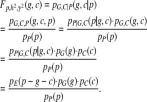(A14)

Note that the move from to is justified since P = G + C + E. Now, in terms of we have

(A15)

Explicitly substituting and simplifying terms, we get the bivariate normal form,

(A16)

We may now employ F to find our conditional probability, Prob(|C| > K | P). This probability is in fact the integral of the distribution of F in the domain that satisfies |C| > K, denoted by . We therefore have

(A17)

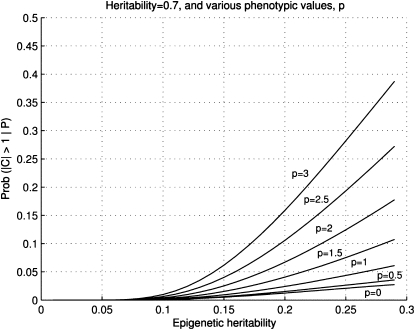
Figure A1 depicts the graphs of M as a function of γ² for various absolute values of P when h² > γ². Note that for a given h², Prob(|C| > K|P) is always higher for a larger |P|, suggesting it is more productive to focus on classes of individuals with larger phenotypic deviations from the population mean.

Figure 4.

Figure A1.—The graphs of M for h² = 0.7. Depicted for various values of the phenotypic deviation (in standard deviations), γ² varies from 0 to 0.3. These are the probabilities that the epigenetic deviation of an individual |C| is at the extremes of its distribution, Prob(|C| > K | P), where K = 1 (in standard deviations of P).

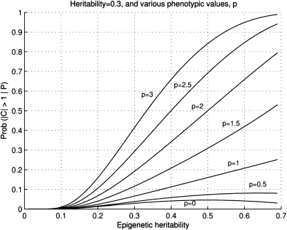
In the case where h² may be <γ² we get a similar increase in probability for larger phenotypic values, as depicted in Figure A2.

Figure 5.

Figure A2.—The graphs of M for h² = 0.3. Depicted for various values of the phenotypic deviation (in standard deviations), γ² varies from 0 to 0.7.

We can now utilize M to assess whether the variance components we have estimated through the familial covariances warrant further molecular investigation. Instead of basing our threshold on an arbitrary value of the epigenetic heritability, we decide on an epigenetic deviation threshold K, typically at one standard deviation (of P), and a probability threshold, T, and plug the epigenetic heritability, the genetic heritability, and a phenotypic deviation into M. If M = Prob(|C | > K |P) > T, then we gain confidence that the heritable epigenetic deviation, |C|, is large enough to warrant looking deeper into organisms with a phenotypic deviation larger than |P|.

References

- Allis, C. D., T. Jenuwein, D. Reinberg and M. L. Caparros (Editors), 2007. Epigenetics. Cold Spring Harbor Laboratory Press, Cold Spring Harbor, NY.
- Anway, M. D., A. S. Cupp, M. Uzumcu and M. K. Skinner, 2005. Epigenetic transgenerational actions of endocrine disruptors and male fertility. Science 308(5727): 1466–1469. [DOI] [PMC free article] [PubMed] [Google Scholar]
- Bonduriansky, R., and T. Day, 2009. Nongenetic inheritance and its evolutionary implications. Annu. Rev. Ecol. Evol. Syst. 40 103–125. [Google Scholar]
- Bossdorf, O., C. L. Richards and M. Pigliucci, 2008. Epigenetics for ecologists. Ecol. Lett. 11(2): 106–115. [DOI] [PubMed] [Google Scholar]
- Boyd, R., and P. J. Richerson, 1985. Culture and the Evolutionary Process. University of Chicago Press, Chicago.
- Brun, J., 1965. Genetic adaptation of Caenorhabditis elegans (Nematoda) to high temperatures. Science 150 1467.5322584 [Google Scholar]
- Cavalli-Sforza, L. L., and M. W. Feldman, 1973. Cultural versus biological inheritance: phenotypic transmission from parents to children (a theory of the effect of parental phenotypes on children's phenotypes). Am. J. Hum. Genet. 25 618–637. [PMC free article] [PubMed] [Google Scholar]
- Cloninger, C. R., J. Rice and T. Reich, 1978. Multifactorial inheritance with cultural transmission and assortative mating. II. A general model of combined polygenic and cultural inheritance. Am. J. Hum. Genet. 31 176–198. [PMC free article] [PubMed] [Google Scholar]
- Falconer, D. S, and T. F. C. Mackay, 1996. Introduction to Quantitative Genetics, Ed. 4. Longmans Green, Harlow, Essex, UK.
- Feldman, M. W, and K. N. Laland, 1996. Gene-culture coevolutionary theory. Trends Ecol. Evol. 11 453–457. [DOI] [PubMed] [Google Scholar]
- Flanagan, J. M., V. Popendikyte, N. Pozdniakovaite, M. Sobolev, A. Assadzadeh et al., 2006. Intra- and interindividual epigenetic variation in human germ cells. Am. J. Hum. Genet. 79 67–84. [DOI] [PMC free article] [PubMed] [Google Scholar]
- Gilbert, S. F., and D. Epel, 2009. Ecological Developmental Biology. Integrating Epigenetics, Medicine, and Evolution. Sinauer Associates, Sunderland, MA.
- Ginsburg, S., and E. Jablonka, 2009. Epigenetic learning in non-neural organisms. J. Biosci. 34 633–646. [DOI] [PubMed] [Google Scholar]
- Grewal, M. S., 1962. The rate of genetic divergence of sublines in the C57BL strain of mice. Genet. Res. 3 226–237. [Google Scholar]
- Hoi-Sen, Y., 1972. Is subline differentiation a continuing process in inbred lines of mice? Genet. Res. 19 53–59. [DOI] [PubMed] [Google Scholar]
- Jablonka, E., 2004. Epigenetic epidemiology. Int. J. Epidemiol. 33(5): 929–935. [DOI] [PubMed] [Google Scholar]
- Jablonka, E., and M. J. Lamb, 1995. Epigenetic Inheritance and Evolution: The Lamarckian Dimension. Oxford University Press, Oxford.
- Jablonka, E., and M. J. Lamb, 2005. Evolution in Four Dimensions: Genetic, Epigenetic, Behavioral, and Symbolic Variation in the History of Life. MIT Press, Cambridge, MA.
- Jablonka, E, and G. Raz, 2009. Transgenerational epigenetic inheritance: prevalence, mechanisms, and implications for the study of heredity and evolution. Q. Rev. Biol. 84(2): 131–176. [DOI] [PubMed] [Google Scholar]
- Jablonka, E., B. Oborny, I. Molnar, E. Kisdi, J. Hofbauer et al., 1995. The adaptive advantage of phenotypic epigenetic transmissibility in changing environments. Philos. Trans. R. Soc. B 350 133–141. [DOI] [PubMed] [Google Scholar]
- Johannes, F., V. Colot and R. C. Jansen, 2008. Epigenome dynamics: a quantitative genetics perspective. Nat. Rev. 9 883–890. [DOI] [PubMed] [Google Scholar]
- Johannes, F., E. Porcher, F. K. Teixeira, V. Saliba-Colombani, M. Simon et al., 2009. Assessing the impact of transgenerational epigenetic variation on complex traits. PLoS Genet. 5(6): e1000530. [DOI] [PMC free article] [PubMed] [Google Scholar]
- Kirkpatrick, M., and R. Lande, 1989. The evolution of maternal characters. Evolution 43 485–503. [DOI] [PubMed] [Google Scholar]
- Lachmann, M., and E. Jablonka, 1996. The inheritance of phenotypes: an adaptation to fluctuating environments. J. Theor. Biol. 181 1–9. [DOI] [PubMed] [Google Scholar]
- Lande, R., 1976. The maintenance of genetic variability by mutation in a polygenic character with linked loci. Genet. Res. 26 221–235. [DOI] [PubMed] [Google Scholar]
- Nadeau, J. H., 2009. Transgenerational genetic effects on phenotypic variation and disease risk. Hum. Mol. Genet. 18 R202–R210. [DOI] [PMC free article] [PubMed] [Google Scholar]
- Pembrey, M. E., L. O. Bygren, G. Kaati, S. Edvinsson, K. Northstone et al., 2006. ALSPAC study team: sex-specific, male-line transgenerational responses in humans. Eur. J. Hum. Genet. 14 159–166. [DOI] [PubMed] [Google Scholar]
- Rao, D. C., N. E. Morton and S. Yee, 1976. Resolution of cultural and biological inheritance by path analysis. Am. J. Hum. Genet. 28 228–242. [PMC free article] [PubMed] [Google Scholar]
- Reinders, J., B. B. Wulff, M. Mirouze, A. Marí-Ordóñez, M. Dapp et al., 2009. Compromised stability of DNA methylation and transposon immobilization in mosaic Arabidopsis epigenomes. Genes Dev. 23 939–950. [DOI] [PMC free article] [PubMed] [Google Scholar]
- Richards, E. J., 2008. Population epigenetics. Curr. Opin. Genet. Dev. 18 221–226. [DOI] [PubMed] [Google Scholar]
- Richerson, P. J., and R. Boyd, 2005. Not by Genes Alone: How Culture Transformed Human Evolution. University of Chicago Press, Chicago.
- Ruden, D. M., M. D. Garfinkel, L. Xiao and X. Lu, 2005. Epigenetic regulation of trinucleotide repeat expansions and contractions and the “biased embryos” hypothesis for rapid morphological evolution. Curr. Genomics 6 145–155. [Google Scholar]
- Ruden, D. M., D. Curtis, C. Jamison, B. R. Zeeberg, M. D. Garfinkel et al., 2008. The EDGE hypothesis: epigenetically directed genetic errors in repeat-containing proteins (RCPs) involved in evolution, neuroendocrine signaling, and cancer. Front. Neuroendocrinol. 29 428–444. [DOI] [PMC free article] [PubMed] [Google Scholar]
- Ruvinsky, A. O., Y. I. Lobkov and D. K. Belyaev, 1983. a Spontaneous and induced activation of genes affecting the phenotypic expression of glucose 6-phosphate dehydrogenase in Daphnia pulex. I. Intraclonal variations in the electrophoretic mobility of G6PD. Mol. Gen. Genet. 189 485–489. [DOI] [PubMed] [Google Scholar]
- Ruvinsky, A. O., Y. I. Lobkov and D. K. Belyaev, 1983. b Spontaneous and induced activation of genes affecting the phenotypic expression of glucose 6-phosphate dehydrogenase in Daphnia pulex. II. Glucose-induced changes in the electrophoretic mobility of G6PD. Mol. Gen. Genet. 189 490–494. [DOI] [PubMed] [Google Scholar]
- Salmon, A., M. L. Ainouche and J. F. Wendel, 2005. Genetic and epigenetic consequences of recent hybridization and polyploidy in Spartina (Poaceae). Mol. Ecol. 14(4): 1163–1175. [DOI] [PubMed] [Google Scholar]
- Shorter, J., and S. L. Lindquist, 2005. Prions as adaptive conduits of memory and inheritance. Nat. Rev. Genet. 6 435–450. [DOI] [PubMed] [Google Scholar]
- Slatkin, M., 2009. Epigenetic inheritance and the missing heritability problem. Genetics 182(3): 845–850. [DOI] [PMC free article] [PubMed] [Google Scholar]
- Tal, O., 2009. From heritability to probability. Biol. Philos. 24 81–105. [Google Scholar]
- Teixeira, F. K., F. Heredia, A. Sarazin, F. Roudier, M. Boccara et al., 2009. A role for RNAi in the selective correction of DNA methylation defects. Science 23 1600–1604. [DOI] [PubMed] [Google Scholar]
- Verhoeven, K. J. F., J. J. Jeroen, P. J. van Dijk and A. Biere, 2009. Stress-induced DNA methylation changes and their heritability in asexual dandelions. New Phytol. 185 1108–1118. [DOI] [PubMed] [Google Scholar]
- Whittle, C. A., S. P. Otto, M. O. Johnston and J. E. Krochko, 2009. Adaptive epigenetic memory of ancestral temperature regime in Arabidopsis thaliana. Botany 87 650–657. [Google Scholar]
- Wolf, J. B., E. D. Brodie, J. M. Cheverud, A. J. Moore and M. J. Wade, 1998. Evolutionary consequences of indirect genetic effects. Trends Ecol. Evol. 13 64–69. [DOI] [PubMed] [Google Scholar]