Mean square exponential and robust stability of stochastic discrete-time genetic regulatory networks with uncertainties

Abstract

This paper aims to analyze global robust exponential stability in the mean square sense of stochastic discrete-time genetic regulatory networks with stochastic delays and parameter uncertainties. Comparing to the previous research works, time-varying delays are assumed to be stochastic whose variation ranges and probability distributions of the time-varying delays are explored. Based on the stochastic analysis approach and some analysis techniques, several sufficient criteria for the global robust exponential stability in the mean square sense of the networks are derived. Moreover, two numerical examples are presented to show the effectiveness of the obtained results.

Introduction

The research of complex dynamical networks varies from biological and chemical oscillators to scientific collaboration networks as well as neurodynamics and biological neural networks (Dorogotsev and Mendes 2003; Becskei and Serrano 2000; Bolouri and Davidson 2002; Wang et al. 2008; Wang and Zhang 2007; Chaouiya 2007). As a special case, genetic regulatory networks (GRNs) consisting of DNA, RNA, proteins, small molecules and their mutual regulatory interactions, have become an important new area of research in the biological and biomedical sciences and received widely attention recently (Becskei and Serrano 2000; Bolouri and Davidson 2002; Weaver et al. 1999; De Jong 2002; Smolen et al. 2000). Several models have been developed to investigate the behaviors of the GRNs, for example, Boolean models (Weaver et al. 1999), the differential equation models (De Jong 2002; Smolen et al. 2000), the Petri net models (Chaouiya 2007) and discrete time piecewise affine model (Lima and Ugalde 2006; Coutinho et al. 2006). Among them, GRNs in the form of differential equation models have been well studied in He and Cao (2008), Ren and Cao (2008), Ribeiro et al. (2006) and Cao and Ren (2008).

It is revealed that time delay, which inevitably exists in GRNs due to slow biochemical reactions such as gene transcription, translation, diffusion, and translocation processes (see Hirata et al. 2002; Lewis 2003), is an important factor and should be considered. Various efforts have been paid in the past few years for the analysis of GRNs with time delay, see He and Cao (2008), Ren and Cao (2008), Chen and Aihara (2002a, b) and Li et al. (2006). In Chen and Aihara (2002), presented a model for GRNs with constant delay and analyzed nonlinear properties of the model in terms of local stability and bifurcation. Subsequently, they explained periodic oscillations which are mainly generated by nonlinearly negative and positive feedback loops in gene regulatory systems, and explored effects of time delay on stability region of the oscillations (see Chen and Aihara 2002). In Li et al. (2006), a nonlinear model for GRNs with SUM regulatory functions was presented and some sufficient conditions for the stability of the GRNs involving time varying delays and stochastic perturbations were derived by using the Lyapunov method and the Lur’e system approach. He and Cao (2008) investigated global asymptotic stability of GRNs with distributed delay. In Ren and Cao (2008), by using the Lyapunov method and linear matrix inequality (LMI) approach, sufficient conditions were proposed to ensure robust asymptotic stability of GRNs with time-varying delays and parameter uncertainties. On the other hand, due to small numbers of transcriptional factors and other key signaling proteins, considerable experimental evidences show that noise plays a very important role in gene regulation (Tian et al. 2007; Jonathan and Erin 2005). In addition, gene expression involves a series of molecular events in cells, which are often subject to significant intrinsic fluctuations and extrinsic disturbances, thus being best viewed as a stochastic process (Jonathan and Erin 2005; Michael et al. 2002; Sun et al. 2009). So the stochastic differential equation model has recently been developed to describe the molecular fluctuation in gene networks (Lestas et al. 2008, Li et al. 2007).

It is worth noting that most references for delayed GRNs were only concerned with the case of deterministic time delay(s). But in many real systems, such as the networked control systems, the network-induced delay often appears as some probabilistic properties and its probability distribution can be measured by the statistical method (Yue et al. 2009). On the other hand, it is shown in Ribeiro et al. (2006) that time delays in some GRNs are often existent in a stochastic fashion. And their probabilistic characteristics can also be obtained by statistical methods. Hence, it is necessary to consider stochastic delay effects in GRNs. In addition, as pointed out in Lima and Ugalde (2006), Coutinho et al. (2006) and Cao and Ren (2008), some GRN models are discrete-time dynamical systems which can be viewed as an extension of discrete-time delay systems and are more important than their continuous-time counterpart in a sense. These kinds of discrete-time models are directly inspired by the systems of differential equations mentioned above, though they do not correspond to a time discretization of the differential equations but rather to a natural discrete-time version of them. Hence, it is clear that theoretical analysis of stability of discrete-time GRNs is an important and necessary step. However, to the best of the author’s knowledge, little attention has been paid to this issue, especially investigation on stability of discrete-time GRNs with stochastic delay when considering the information of both variation range and probability distribution of the time delay.

In this paper, we aim to solve the problem of global robust exponential stability in the mean square sense (GRES-MSE) of discrete-time GRNs with parameter uncertainties and stochastic disturbances. The parameter uncertainties are assumed to be norm-bounded and the stochastic disturbances are described in terms of a Brownian motion. By using two stochastic variables which satisfy Bernoulli random binary distribution, we construct a new model of discrete-time GRNs with stochastic time-varying delays. Then some sufficient conditions for GRES-MSE of the stochastic discrete-time GRNs with uncertainties are exploited. It should be noted that the solvability of the derived conditions depends on not only the size of the delay but also the probability of the delay appearing in some intervals. Numerical examples are presented to show the effectiveness and applicability of the proposed results.

Notations Throughout this paper, denotes the n-dimensional Euclidean space. is the set of real n × m matrices. I is the identity matrix of the appropriate dimensions. ||·|| stands for the Euclidean vector norm or spectral norm as appropriate. diag(·) denotes a diagonal matrix. The superscript “T” represents the matrix transposition. The notation X > 0 (respectively, X ≥ 0) for means that the matrix X is positive definite (respectively, positive semidefinite). stands for the expectation. [a, b] denotes a set involving all integers between a and b. and denote the minimum and maximum eigenvalue of the real symmetric matrix P. In symmetric block matrices, the symbol “*” is used as an ellipsis for terms induced by symmetry. denotes the set including zero and positive integers. denotes the empty set. is a probability space, where Ω is the sample space, is the -algebra of subsets of the sample space and is the probability measure on .

Model description and preliminaries

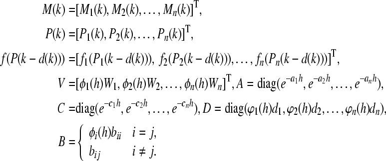
Consider a discrete-time GRN with variable delays containing of n mRNAs and n proteins can be formulated by the following difference equation

1

This mathematical model is taken from Cao and Ren (2008) with slack variation on time delays, where and are the concentrations of mRNA and protein of the ith gene; h is a fixed positive real number denoting a uniform discretionary step size; a_i > 0 and c_i > 0 are the degradation rates of mRNA and protein, respectively; d_i is the translation rate; d(k) > 0 and τ(k) > 0 denote random time delays for mRNAs and Proteins, respectively; where ν_ij is the bounded constant and denotes the dimensionless transcriptional rate of transcription factor j to i, and is the set of all the j genes; and . Obviously, ϕ_i(h) > 0, φ_i(h) > 0. The coupling coefficient b_ij (i, j = 1, 2, ..., n) is defined as follows:

2

In addition, the nonlinear function represents the feedback regulation of the protein on the transcription. It is a monotonic function in Hill form, that is, (j = 1, 2, ..., n), where h_j is the Hill coefficient.

Let us rewrite system (1) into the following compact matrix form

3

where

Let be an equilibrium point of system (3). Then it satisfies

4

For convenience, let us shift an intended equilibrium point of system (3) to the origin through the transformations x(k) = M(k) − M*, y(k) = P(k) − P*. Then system (3) can be transformed into

5

where g(y(k)) = f(y(k) + P*) − f(P*).

As mentioned before, little study has been performed on GRNs when considering unavoidable uncertainties or external perturbations, but in the applications and designs of networks, such as genetic networks and neural networks, there are often some unavoidable uncertainties such as modeling errors, external perturbations, and parameter fluctuations, which may cause the networks to be unstable. Hence, it is essential to take into account parameter uncertainties and stochastic disturbance additionally as studied in Ren and Cao (2008) and Li et al. (2007). A general GRN model containing these influences can be described as follows

6

where ΔA(k), ΔB(k), ΔC(k) and ΔD(k) denote the parameter uncertainties satisfying the following condition

where H, E₁, E₂, E₃ and E₄ are constant matrices of appropriate dimensions, and F(k) is an unknown time-varying matrix satisfying F^T(k)F(k) ≤ I. represents a noise intensity function vector; w(k) is a scalar Wiener process on a probability space with

Assumption 1 For i ∈ {1, 2, ..., n}, each function g_i(·) is continuous and bounded, and satisfies that

where l_i and L_i are known constants.

Remark 1 The constants l_i and L_i here are allowed to be positive, negative, or zero, which makes this assumption on function g(·) less conservative than those stated in He and Cao (2008), Ren and Cao (2008), Chen and Aihara (2002a, b) and Li et al. (2006).

Assumption 2 Suppose that

where H₁ > 0 and H₂ > 0 are two known matrices.

Assumption 3 Suppose that the time-varying delays d(k) and τ(k) are bounded with 0 < d_m ≤ d(k) ≤ d_M, 0 < τ_m ≤ τ(k) ≤ τ_M, and their probability distributions can be observed.

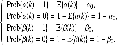
Remark 2 In what follows, in order to transform system (6) with random delays d(k) and τ(k) into an equivalent system which dependents on distributed sequences, similar analysis as exploited in Yue et al. [2008, 2009] can also be carried out for the random delays. Suppose that d(k) takes values in [d_m, d₀] or (d₀, d_M] and , where d₀, d_m, d_M are integers satisfying d_m ≤ d₀ < d_M, and 0 ≤ α₀ ≤ 1. Similarly, τ(k) takes values in [τ_m, τ₀] or (τ₀, τ_M] and , where τ₀, τ_m, τ_M are integers satisfying τ_m ≤ τ₀ < τ_M, and 0 ≤ β₀ ≤ 1.

Define four sets , , and . Obviously, , , and . Furthermore, define four mapping functions

and

Then one can define two stochastic variables α(k) and β(k) which are Bernoulli distributed white sequences taking the values of 0 and 1 with

Therefore, system (6) can be equivalently rewritten as

7

For brevity of the following analysis, denote x(k), y(k), α(k), 1 − α(k), β(k), 1 − β(k), w(k), τ₁(k), τ₂(k), x(k − τ₁(k)), x(k − τ₂(k)), d₁(k), d₂(k), g(y(k − d₁(k))), g(y(k − d₂(k))), ΔA(k), ΔB(k), ΔC(k) and ΔD(k) by x_k, y_k, α_k, , β_k, , w_k, τ^k₁, τ^k₂, x_τ,1, x_τ,2, d^k₁, d^k₂, g(y_d,1), g(y_d,2), ΔA_k, ΔB_k, ΔC_k and ΔD_k, respectively.

Then system (7) can be rewritten as

8

Remark 3 It should be pointed out that, up to now, most existing literatures concentrate on the stability of continuous-time GRNs, but few attempts are devoted to the problem of stability of discrete-time GRNs with stochastic delays. Although the introduction of binary stochastic variables has been presented in the Wang et al. (2006, 2004) and then developed in Yue et al. (2008, 2009), the stability problem for GRNs with stochastic delays still remains challenging.

Definition 1 The origin of system (8) is said to be globally robustly exponentially stable in the mean square sense with w_k = 0, if there exist constants γ > 0 and 0 < σ < 1 such that every solution of system (8) for all parameter uncertainties (that is, ΔA_k, ΔB_k, ΔC_k and ΔD_k) satisfies

Lemma 1 (Schur complement) (Mahmoud and Shi 2003) Given constant matrices Ω₁, Ω₂, Ω₃, where Ω₁ = Ω^T₁ and 0 < Ω₂ = Ω^T₂, then Ω₁ + Ω^T₃Ω⁻¹₂Ω₃ < 0 if and only if

Lemma 2 For any vectors a, b ∈ Rⁿ, the inequality

holds, in which Y is any matrix with Y > 0.

Proof Since Y > 0, we have

This completes the proof.□

Main results

In this section, we shall derive sufficient conditions for mean square exponential robust stability of stochastic discrete-time GRNs with random delays. The main results will be stated in two parts.

Case I GRNs without parameter uncertainties.

Firstly, consider the following stochastic GRNs without parameter uncertainties

9

For simplifying the following representation, denote

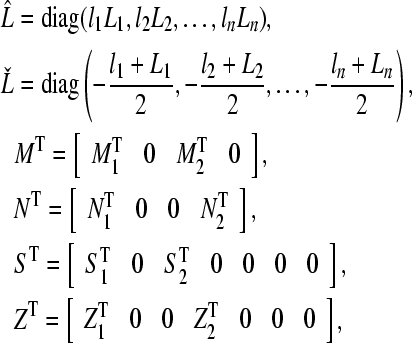where M_i, N_i, S_i and Z_i (i = 1, 2) are any matrices with appropriate dimensions.

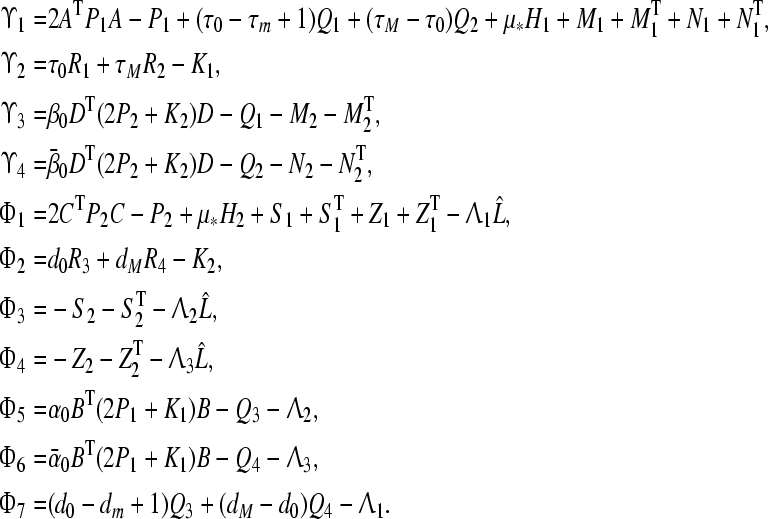
Theorem 1 The origin of system (9) is said to be globally exponentially stable in the mean square sense if there exist three positive diagonal matrices , positive definite matrices P₁, P₂, Q₁, Q₂, Q₃, Q₄, R₁, R₂, R₃, R₄, K₁, K₂, any matrices M₁, M₂, N₁, N₂, S₁, S₂, Z₁, Z₂ of appropriate dimensions and a positive scalar μ_* > 0 such that the following LMIs

10

11

12

hold, where

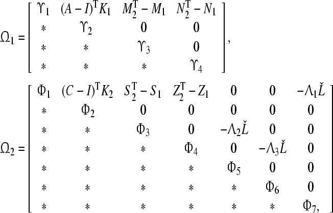with

Proof See Appendix A.□

Case II GRNs with parameter uncertainties. In this part, we consider the stochastic GRN (8) with parameter uncertainties.

Theorem 2 The origin of system (8) is said to be globally robustly exponentially stable in the mean square sense if there exist three positive diagonal matrices , positive definite matrices P₁, P₂, Q₁, Q₂, Q₃, Q₄, R₁, R₂, R₃, R₄, K₁, K₂, any matrices M₁, M₂, N₁, N₂, S₁, S₂, Z₁, Z₂ of appropriate dimensions and scalars μ_* > 0, k_i > 0 (i = 1, ..., 6) such that the following LMIs

13

14

15

hold, where

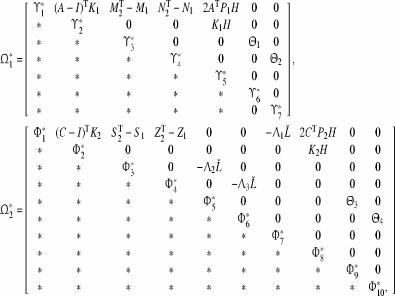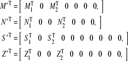with

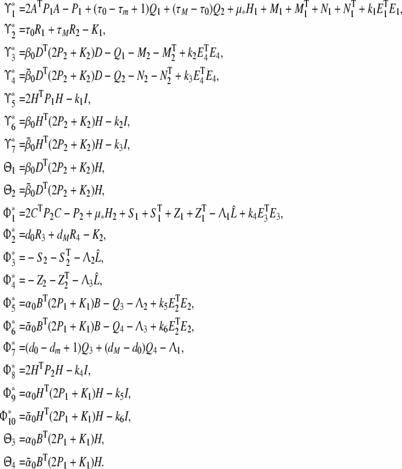Proof See Appendix B.□

Examples

In this section, two numerical examples are presented to illustrate the applicability and effectiveness of our results.

Example 1 Consider a two-node GRN (9) with the following parameters:

Here, suppose τ_m = 1, τ₀ = 3, d_m = 1, d₀ = 3. It can be calculated that , By setting α₀ = 0.8, β₀ = 0.6, τ_M = 7, d_M = 10 in Theorem 1 and using Matlab LMI toolbox, a set of one feasible solutions of LMIs (10)- (12) can be obtained as follows:

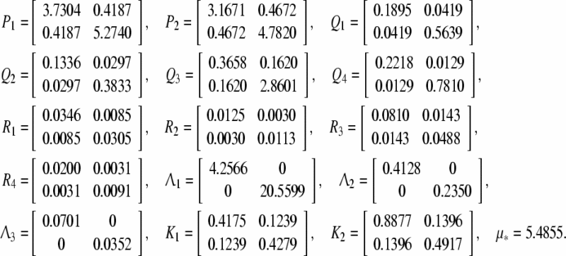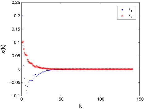
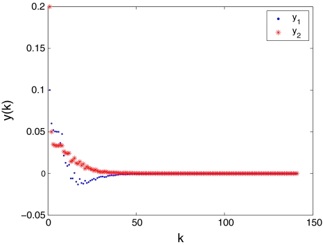
Therefore, all the conditions in Theorem 1 are satisfied, which indicates that the origin of system (9) with stochastic delays and disturbances is globally exponentially stable in the mean square sense. Computer simulations for transient responses of state variables x_k and y_k in system (9) are depicted in Figs. 1 and 2, respectively.

Fig. 1.

Transient responses of state variables x_k in system (9)

Fig. 2.

Transient responses of state variables y_k in system (9)

Example 2 Consider another five-node GRN (8) with the following parameters:

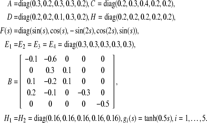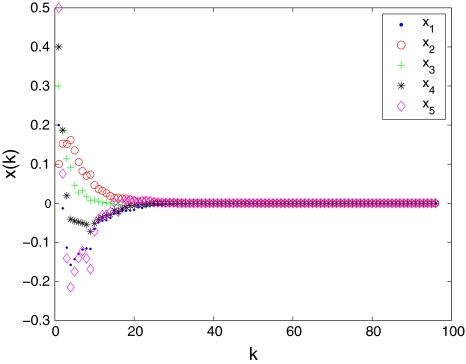
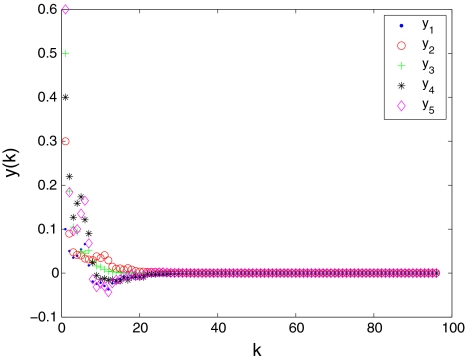
It is easy to obtain that , Set τ_m = 1, τ₀ = 4, τ_M = 8, d_m = 1, d₀ = 3, d_M = 10, α₀ = 0.6, β₀ = 0.7. By applying Theorem 2, one can verify by Matlab LMI toolbox that feasible solutions of the LMIs (13–15) exist. Therefore, for all parameter uncertainties and stochastic perturbations, the origin of system (8) is said to be globally robustly exponentially stable in the mean square sense. Computer simulations for transient responses of state variables x_k and y_k in system (8) are shown in Figs. 3 and 4, respectively.

Fig. 3.

Transient responses of state variables x_k in system (8)

Fig. 4.

Transient responses of state variables y_k in system (8)

Conclusions

The problem of global robust exponential stability of stochastic discrete-time GRNs with parameter uncertainties and random delays has been studied. By constructing a proper Lyapunov-Krasovskii functional and adopting a new modelling method, two delay-distribution-dependent conditions are derived. Different from the existing GRN models, the probability distributions of the time delays have been translated into the networks’ parameter matrices. Two numerical examples and their simulations have been given to illustrate the effectiveness and applicability of the obtained results.

Appendix A: Proof of Theorem 1

Consider the following Lyapunov-Krasovskii functional candidate:

16

where

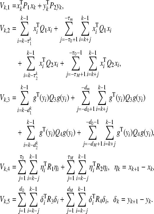Calculating the difference of V_k along the solution of (9) and taking its mathematical expectation yield

17

18

19

20

21

Considering Assumption 2 and (10), it can be easily obtained

22

Making use of Lemma 2, we can derive

23

24

25

26

Obviously, the following zero equations hold.

27

28

29

30

where

By applying Lemma 2, we have

31

32

33

34

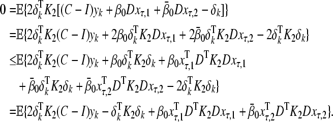
For positive definite matrices K₁ and K₂, it follows from the definition of η_k and δ_k that

35

36

Taking the expectations on both side of (35) and (36), and employing Lemma 2 yield

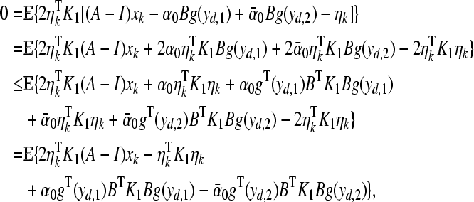37

and

38

In view of Assumption 1, we can conclude that

39

40

41

It can be deduced from (39) that there exists a diagonal matrix such that

42

where e_i denotes a column vector having “1” element on its ith row and zeros elsewhere. Similarly, by means of (40) and (41), there exist diagonal matrices and such that

43

and

44

respectively.

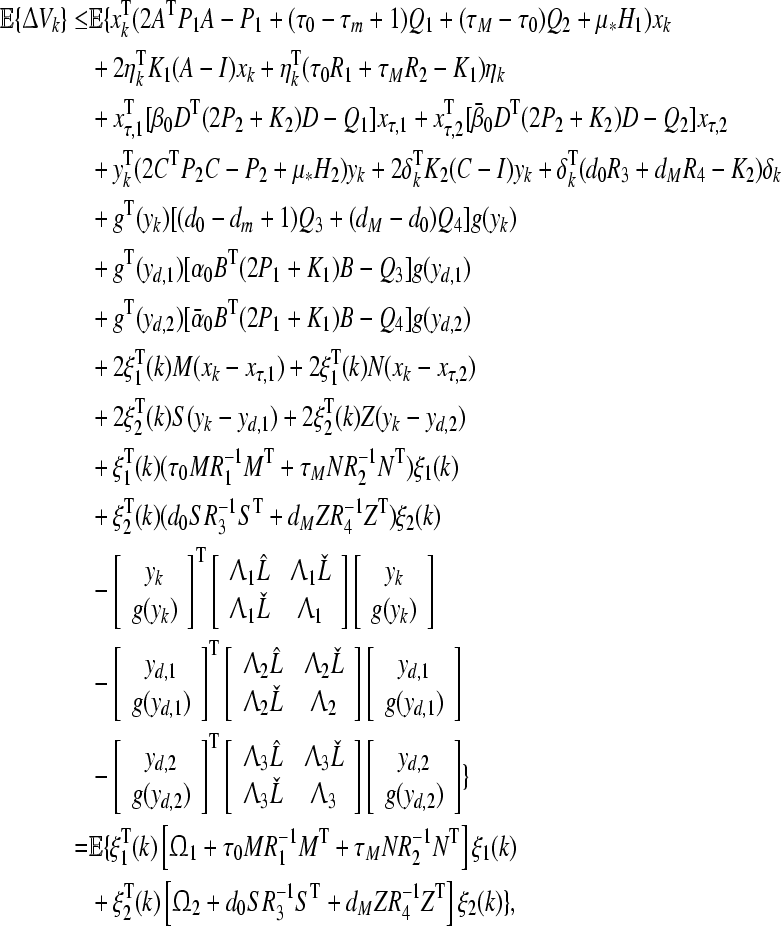
Therefore, we have

45

where

According to the well-known Schur complement (see, Lemma 1), one can get

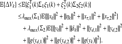In view of the conditions Σ₁ < 0 and Σ₂ < 0 in Theorem 1, it follows that

46

which implies that the origin of system (9) is globally asymptotically stable in the mean square sense.

Now, we are in a position to proceed with the global exponential stability analysis of the system (9). It follows from Assumption 1 that

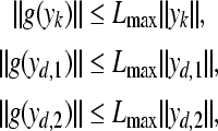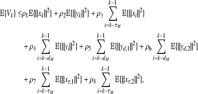
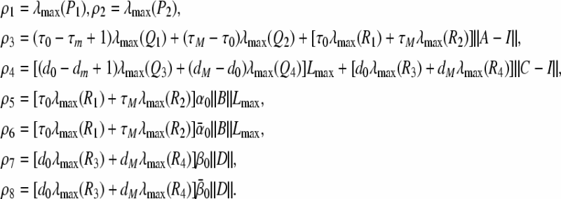
where L_max = max{|l₁|, ..., |l_n|, |L₁|, ..., |L_n|}. Based upon expression of V_k, one can get

47

where

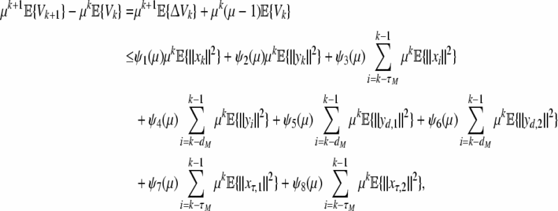
For any scalar μ > 1, the above inequality (47), together with (46), implies that

48

where and ψ_j(μ) = (μ − 1)ρ_j, j = 3, ..., 8.

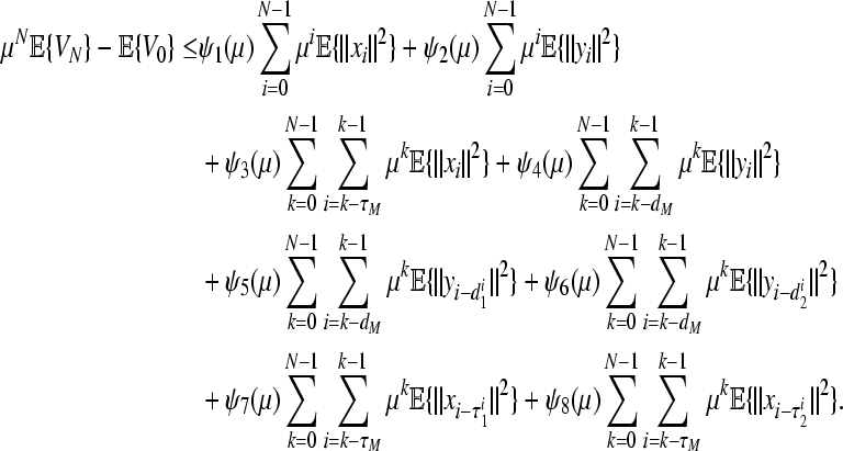
Furthermore, for any integer N ≥ 1, summing up both sides of (48) from 0 to N − 1 with respect to k, yields

49

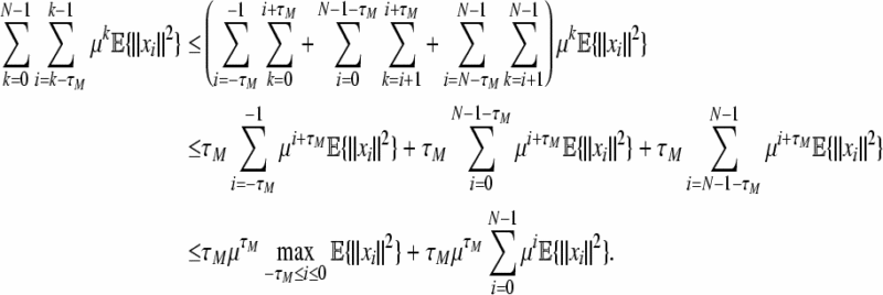
Note that for τ_M ≥ 1. It follows that

50

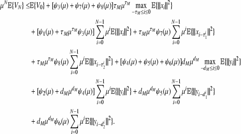
Hence, Eq. (49) can be written as

51

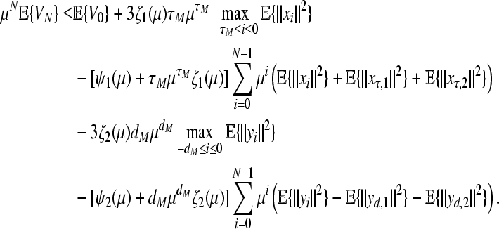
Let σ₁ = max{ρ₃, ρ₇, ρ₈}, ζ₁(μ) = (μ − 1)σ₁, σ₂ = max{ρ₄, ρ₅, ρ₆} and ζ₂(μ) = (μ − 1)σ₂. It follows from (51) that

52

Define Note that it can be verified that there exists a scalar θ > 1 such that Φ(θ) = 0. Therefore, for such a scalar θ, we have

53

Meanwhile, one can derive from (47) that

54

Substituting (54) into (53) yields

55

On the other hand, from (16), it is easy to obtain

56

where

Combining (55) and (56), one can get

57

yielding

58

where

Since N is an any positive integer, it can be concluded from Definition 1 that the origin of system (9) is globally exponentially stable in the mean square. This completes the proof of the theorem. □

Appendix B: Proof of Theorem 2

Consider the same Lyapunov–Krasovskii functional as that in the proof of Theorem 1. Then replace A, B, C and D in Theorem 1 by A + HF(k)E₁, B + HF(k)E₂, C + HF(k)E₃ and D + HF(k)E₄, respectively.

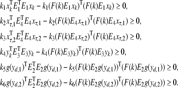
Since F^T(k)F(k) ≤ I, it follows that

59

Calculating together with the above inequalities, we obtain

where

The remaining proof for global robust exponential stability is similar to those in the proof of Theorem 1. For the sake of simplicity, we omit it here. □

References

- Becskei A, Serrano L. Engineering stability in gene networks by autoregulation. Nature. 2000;405(6786):590–593. doi: 10.1038/35014651. [DOI] [PubMed] [Google Scholar]
- Bolouri H, Davidson EH. Modeling transcriptional regulatory networks. BioEssays. 2002;24(12):1118–1129. doi: 10.1002/bies.10189. [DOI] [PubMed] [Google Scholar]
- Cao JD, Ren FL. Exponential stability of discrete-time genetic regulatory networks with delays. IEEE Trans Neural Networks. 2008;19(3):520–523. doi: 10.1109/TNN.2007.911748. [DOI] [PubMed] [Google Scholar]
- Chaouiya C. Petri net modelling of biological networks. Brief Bioinform. 2007;8:210–219. doi: 10.1093/bib/bbm029. [DOI] [PubMed] [Google Scholar]
- Chen LN, Aihara K. Stability of genetic regulatory networks with time delay. IEEE Trans Circuits Syst I. 2002;49(5):602–608. doi: 10.1109/TCSI.2002.1001949. [DOI] [Google Scholar]
- Chen LN, Aihara K. A model of periodic oscillation for genetic regulatory systems. IEEE Trans Circuits Syst I. 2002;49(10):1429–1436. doi: 10.1109/TCSI.2002.803354. [DOI] [Google Scholar]
- Coutinho R, Fernandez B, Lima R, et al. Discrete time piecewise affine models of genetic regulatory networks. J Math Biol. 2006;52(4):524–570. doi: 10.1007/s00285-005-0359-x. [DOI] [PubMed] [Google Scholar]
- De Jong H. Modeling and simulation of genetic regulatory systems: a literature review. J Comput Biol. 2002;9(1):67–103. doi: 10.1089/10665270252833208. [DOI] [PubMed] [Google Scholar]
- Dorogotsev SN, Mendes JFF. Evolution of networks: from biological nets to the internet and WWW. Oxford: Oxford University Press; 2003. [Google Scholar]
- He WL, Cao JD. Robust stability of genetic regulatory networks with distributed delay. Cogn Neurodyn. 2008;2(4):355–361. doi: 10.1007/s11571-008-9062-0. [DOI] [PMC free article] [PubMed] [Google Scholar]
- Hirata H, Yoshiura S, Ohtsuka T, et al. Oscillatory expression of the bHLH factor Hes1 regulated by a negative feedback loop. Science. 2002;298(5594):840–843. doi: 10.1126/science.1074560. [DOI] [PubMed] [Google Scholar]
- Jonathan MR, Erin KO. Noise in gene expression: origins, consequences, and control. Science. 2005;309(5743):2010–2013. doi: 10.1126/science.1105891. [DOI] [PMC free article] [PubMed] [Google Scholar]
- Lestas I, Paulsson J, Ross NE, et al. Noise in gene regulatory networks. IEEE Trans Automat Contr. 2008;53:189–200. doi: 10.1109/TAC.2007.911347. [DOI] [Google Scholar]
- Lewis J. Autoinhibition with transcriptional delay: a simple mechanism for the zebrafish somitogenesis oscillator. Curr Biol. 2003;13(16):1398–1408. doi: 10.1016/S0960-9822(03)00534-7. [DOI] [PubMed] [Google Scholar]
- Li CG, Chen LN, Aihara K. Stability of genetic networks with SUM regulatory logic: Lur’e system and LMI approach. IEEE Trans Circuits Syst I. 2006;53(11):2451–2458. doi: 10.1109/TCSI.2006.883882. [DOI] [Google Scholar]
- Li CG, Chen LN, Aihara K. Stochastic stability of genetic networks with disturbance attenuation. IEEE Trans Circuits Syst II. 2007;54(10):892–896. doi: 10.1109/TCSII.2007.901631. [DOI] [Google Scholar]
- Lima R, Ugalde E. Dynamical complexity of discrete-time regulatory networks. Nonlinearity. 2006;19(1):237–259. doi: 10.1088/0951-7715/19/1/012. [DOI] [Google Scholar]
- Mahmoud MS, Shi P. Robust stability, stabilization and H∞ control of time-delay systems with Markovian jump parameters. Int J Robust Nonlinear Contr. 2003;13(8):755–784. doi: 10.1002/rnc.744. [DOI] [Google Scholar]
- Michael BE, Arnold JL, Eric DS, et al. Stochastic gene expression in a single cell. Science. 2002;297(5584):1183–1186. doi: 10.1126/science.1070919. [DOI] [PubMed] [Google Scholar]
- Ren FL, Cao JD. Asymptotic and robust stability of genetic regulatory networks with time-varying delays. Neurocomputing. 2008;71(4-6):834–842. doi: 10.1016/j.neucom.2007.03.011. [DOI] [Google Scholar]
- Ribeiro A, Zhu R, Kauffman SA. A general modeling strategy for gene regulatory networks with stochastic dynamics. J Comput Biol. 2006;13(9):1630–1639. doi: 10.1089/cmb.2006.13.1630. [DOI] [PubMed] [Google Scholar]
- Smolen P, Baxter DA, Byrne JH. Mathematical modeling of gene networks. Neuron. 2000;26(3):567–580. doi: 10.1016/S0896-6273(00)81194-0. [DOI] [PubMed] [Google Scholar]
- Sun YH, Feng G, Cao JD. Stochastic stability of Markovian switching genetic regulatory networks. Phys Lett A. 2009;373(18-19):1646–1652. doi: 10.1016/j.physleta.2009.03.017. [DOI] [Google Scholar]
- Tian T, Burragea K, Burragea PM, et al. Stochastic delay differential equations for genetic regulatory networks. J Comput Appl Math. 2007;205(2):696–707. doi: 10.1016/j.cam.2006.02.063. [DOI] [Google Scholar]
- Wang RB, Zhang ZK. Energy coding in biological neural network. Cogn Neurodyn. 2007;1(3):203–212. doi: 10.1007/s11571-007-9015-z. [DOI] [PMC free article] [PubMed] [Google Scholar]
- Wang ZD, Ho DWC, Liu XH. Robust filtering under randomly varying sensor delay with variance constraints. IEEE Trans Circuits Syst II. 2004;51(6):320–326. doi: 10.1109/TCSII.2004.829572. [DOI] [Google Scholar]
- Wang ZD, Yang FW, Ho DWC, et al. Robust H∞ filtering for stochastic time-delay systems with missing measurements. IEEE Trans Signal Process. 2006;54(7):2579–2587. doi: 10.1109/TSP.2006.874370. [DOI] [Google Scholar]
- Wang RB, Zhang ZK, Chen GR. Energy function and energy evolution on neural population. IEEE Trans on Neural Networks. 2008;19(3):535–538. doi: 10.1109/TNN.2007.914177. [DOI] [PubMed] [Google Scholar]
- Weaver DC, Workman CT, Storm GD. Modeling regulatory networks with weight matrices. Pac Symp Biocomput. 1999;4:112–123. doi: 10.1142/9789814447300_0011. [DOI] [PubMed] [Google Scholar]
- Yue D, Zhang YJ, Tian EG, et al. Delay-distribution-dependent exponential stability criteria for discrete-time recurrent neural networks with stochastic delay. IEEE Trans Neural Networks. 2008;19(7):1299–1306. doi: 10.1109/TNN.2008.2000166. [DOI] [Google Scholar]
- Yue D, Zhang YJ, Tian EG, et al. Delay-distribution-dependent robust stability of uncertain systems with time-varying delay. Int J Robust Nonlinear Contr. 2009;19(4):377–393. doi: 10.1002/rnc.1314. [DOI] [Google Scholar]