Investigating the Effect of Social Changes on Age-Specific Gun-Related Homicide Rates in New York City During the 1990s

Abstract

Objectives. We assessed whether New York City's gun-related homicide rates in the 1990s were associated with a range of social determinants of homicide rates.

Methods. We used cross-sectional time-series data for 74 New York City police precincts from 1990 through 1999, and we estimated Bayesian hierarchical models with a spatial error term. Homicide rates were estimated separately for victims aged 15–24 years (youths), 25–34 years (young adults), and 35 years or older (adults).

Results. Decreased cocaine consumption was associated with declining homicide rates in youths (posterior median [PM] = 0.25; 95% Bayesian confidence interval [BCI] = 0.07, 0.45) and adults (PM = 0.07; 95% BCI = 0.02, 0.12), and declining alcohol consumption was associated with fewer homicides in young adults (PM = 0.14; 95% BCI = 0.02, 0.25). Receipt of public assistance was associated with fewer homicides for young adults (PM = –104.20; 95% BCI = –182.0, –26.14) and adults (PM = –28.76; 95% BCI = –52.65, –5.01). Misdemeanor policing was associated with fewer homicides in adults (PM = –0.01; 95% BCI = –0.02, –0.001).

Conclusions. Substance use prevention policies and expansion of the social safety net may be able to cause major reductions in homicide among age groups that drive city homicide trends.

Most large US cities experienced a decline in homicide during the 1990s. However, nowhere was the decline more publicized than in New York City.^1–4 The city's homicide drop in the 1990s was the largest in its postwar history¹: homicides declined from 2245 in 1990 to 633 in 1998—a drop of 72% over 8 years.²

Two leading theoretical perspectives have guided interpretations of the mechanisms behind New York City's decline in homicide. One of the most prominent theoretical perspectives is the theory of “broken windows” policing,⁵ which proposes that failure to control minor offenses creates a sense of public disorder and encourages the proliferation of crime. This theory motivated investment in increased policing of misdemeanors during the 1990s. Research studying this approach's impact on homicide have produced conflicting evidence; studies exist that report no evidence of reduced homicide associated with misdemeanor policing,^6,7 modest reductions in homicide,^3,4,8 and significant reductions in crime.^9,10

The second theoretical framework, the “crack cocaine” thesis, attributed the increase in homicide in the 1980s to the appearance of crack cocaine in the drug markets of large cities.^11–13 This phenomenon was accompanied by heavy recruitment of young male dealers, creating an increased need for use of guns. Blumstein proposed that the drop in homicide in the 1990s was caused by shifting drug markets, police response to gun carrying by young men, efforts to decrease general access to guns, an increase in the prison population, and economic expansion.^11,12

Previous studies of the determinants of the New York City homicide decline have built on these theoretical perspectives and used pooled cross-sectional time-series designs, as well as natural experiments, to investigate the impact on overall homicide rates of the following phenomena: improvement in policing of low-level, quality-of-life offenses^{3,4,9,10,14,15}; a decline in drug-market activity, with fewer turf wars between drug-dealing crews^{11,12,16–18}; reduced firearm availability as a result of federal and city-level efforts to limit access to and licensing of handguns and assault weapons^16,19,20; the removal of dangerous persons from the streets via implementation of proincarceration policies^15,16,21,22; and a decline in alcohol consumption after the instatement of a consumption tax on beer and hard liquor.²

Previous time-series analyses^3,4,8 have examined the influence of these social determinants on overall homicide, and the current study expands upon that literature by separately examining how such factors are related to homicide victimization in specific age groups. The risk of homicide varies sharply by age,^23–25 and homicide rates in different age groups may result from different sets of risk factors. Indeed, the differential response to social changes by age group may have contributed to the significant shift in the age structure of homicide in the United States in the 20th century.^15,26,27 In New York City, the dramatic drop in homicides in the 1990s benefited some age groups more than others^2,28: adolescents aged between 16 and 19 years and young adults aged 20 to 29 years experienced the sharpest decreases in homicide of all age groups.

Focusing on age-specific rates rather than on overall population rates may allow us to understand the drivers of the homicide rates for the age groups that are causing the overall rates to rise and fall. Therefore, in this analysis, we replicated the pooled, cross-sectional time-series design used in previous studies of the overall homicide rate to compare how social determinants of changes in total homicide levels in New York City (i.e., misdemeanor policing, cocaine consumption, firearm availability, incarceration rates, and alcohol consumption) influenced age-specific gun-related homicide rates in the 1990s.

METHODS

We collected data from 5 sources: the Office of the Chief Medical Examiner (OCME) of New York City, the New York City Police Department (NYPD), the New York City Human Resources Administration, the New York City Mayor's Management Office, and the US Census Bureau. The units of analysis used for this research were New York City police precincts. Precincts are the most appropriate unit of analysis to study the impact of broken-windows policing, because law enforcement is organized at the precinct level.¹⁹ Precincts 33 and 34 were treated as 1 precinct because they were a single precinct until they were split in 1994. The Central Park precinct (precinct 22) was excluded because no one resides in this precinct.

Homicide Measures

We measured gun-related homicide rates for the following age groups of victims: 15 through 24 years, 25 through 34 years, and 35 years and older. These groups were chosen to capture different developmental stages (youth, young adulthood, and adulthood, respectively) and groups at varying risks of homicide; the risk of homicide decreases from its peak at the age group 15–24 years. Models were estimated separately for gun-related homicides for each age group. We focused on gun-related homicides because (1) previous research has demonstrated distinct trends for gun versus nongun homicide in New York City, and (2) the overall trend for gun-related homicide is more compatible with theoretical arguments about the impact of changes in policing and cocaine markets.¹

All cases of homicides in New York City from 1990 to 1999 were identified through standard manual review and abstraction of the medical files of the OCME. The OCME investigates all deaths of people believed to have died from unnatural causes. Thus, all homicide deaths in New York City are reviewed by the OCME and were included in the charts used for data extraction. The same person has held the office of New York City Chief Medical Examiner since 1990, so classification of cases, toxicology, policies, and other aspects of the OCME's work have remained the same over the study period.

Data regarding cause of death, circumstances of death (including use of a gun), and toxicology were collected from the OCME files by trained abstractors using standard protocols and data-collection forms. The OCME investigators used the decedent's medical history, the circumstances and environment of the death, autopsy findings, and laboratory data to attribute the cause of death for each case reviewed. We used ArcGIS version 9.0 (ESRI, Redlands, CA) to geocode all OCME cases from 1990 through 1999 to a precinct by address of injury. Only cases with a valid address of injury were included in the analysis. We used data from the 1990 US Census (summary tape files 1 and 3)²⁹ and the 2000 US Census (summary files 1 and 3)³⁰ to calculate homicide rates per 100 000 population. The total annual precinct population was estimated through linear interpolation for the years between census population estimates of 1990 and 2000.

Other Variable Measures

Data were collected from the NYPD on all misdemeanor/ordinance arrests and citizen complaints by precinct from 1990 through 1999 to represent “broken windows”—oriented policing net of misdemeanor behavior. The misdemeanor–ordinance arrest rate per 10 000 population was used as the predictor of interest, and the rate of complaints per 10 000 population was used as a covariate to adjust for a potential endogenous response to underlying levels of crime.

The proxy measure for cocaine use was the percentage of deaths in each precinct per year from 1990 through 1999 that were classified as accidental by the OCME and that had positive toxicology results for cocaine, recorded from OCME data. We used the annual percentage of gun suicide deaths from 1990 through 1999, recorded from OCME data, as a proxy for precinct firearm availability. This measure correlates highly with survey-based measures of firearm availability.³¹ Incarceration rate per 100 000 population was operationalized as the number of prison admissions by precinct of arrest from 1990 through 1999. This measure was originally obtained from the New York State Division of Criminal Justice Services. Alcohol consumption per precinct was measured as the annual percentage of accidental deaths with toxicology results positive for alcohol from 1990 through 1999, recorded from OCME data.

Potential Confounders

The selection of control variables was informed by previous research by Messner et al.³ and others.³² Time-varying covariates included: the ratio of felony arrests to number of felony complaints from 1990 through 1999, to assess whether increased police activity at all levels rather than increased broken-windows policing specifically was responsible for the decline in homicides²; police manpower, measured as the number of police officers assigned to each police precinct from 1990 through 1999 by the NYPD³; and receipt of public assistance, obtained from the Human Resources Administration at the community–district level and disaggregated to the precinct, as a measure of time-varying neighborhood disadvantage.^33–36

Covariates only available for decennial years and measured as fixed at 1990 were percentage male, percentage under age 35 years, percentage Black, percentage Hispanic, percentage foreign-born, percentage unemployed, and concentrated poverty. These data were obtained from Census Summary File 3.²⁹ Infoshare Online (http://www.infoshare.org) provided census data at the tract level, which were aggregated to the precinct level. We conducted principal component analysis to construct the composite measure of baseline concentrated poverty by summing the percentage of persons living below 200% of the poverty line (to account for the high cost of living in New York City), the percentage with less than a high school education, and the percentage of female-headed households, each weighted by its factor loading. Higher scores indicated greater levels of concentrated poverty. All time-invariant control variables were standardized to a mean of zero and a standard deviation of 1 to improve convergence and to enhance comparability and ease of interpretation.

Statistical Analyses

All analyses were based on “change” Bayesian hierarchical models, which are traditionally used in disease mapping.^37,38 Models took the following forms:

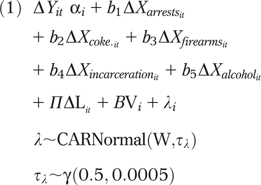where ΔY_it was the change in the age-specific homicide rate between times t and t + 1 for precinct i for time period t, ΔX_arrestsit was the change in the misdemeanor arrest rate between times t and t + 1, ΔX_coke·it was the change in proportion of accident decedents positive for cocaine toxicology, ΔX_firearmsit was the change in the proportion of gun suicides, ΔX_{incarcerationit} was the change in the incarceration rate, ΔX_alcoholit was the change in the proportion of accident decedents positive for alcohol toxicology, ΔL_it was a vector of time-varying covariates, V_i was a set of baseline covariates, and λ_i was the random spatially structured effect.³⁹ We used spatial error models to account for the spatial dependence of risk for homicide in nearby areas. The spatial random effect was modeled with a prior that has a conditionally autoregressive (CAR) distribution, with weights for first-order adjacent neighbors set at 1 (“neighbors” defined as precincts sharing a border).⁴⁰ All models were estimated with Winbugs version 1.2 (MRC Biostatics Unit, Cambridge, England), with 2 parallel Markov chain Monte Carlo chains. Details about these spatial models are given in Appendix 1 (available as a supplement to the online version of this article at http://www.ajph.org).

The predictors of neighborhood homicide rates were examined separately for each homicide victim age group (15–24 years, 25–34 years, 35 years or older). For each age group, a model including the exposures of theoretical interest was first estimated. Next, the time-varying control variables were introduced into the model. Finally, spatial lags for the distribution of significant age-specific predictors in adjacent neighborhoods were included in model 4.

RESULTS

Of 14 186 homicides that occurred in New York City between 1990 and 1999, 2027 (14.3%) were missing precinct-of-injury information, leaving 12 159 homicides classified by precinct of injury. Of these, 8820 (72.5%) were firearm-related and were used in the analysis. Compared to those included in the analysis, firearm homicide decedents who were excluded from the analysis because of missing precinct of injury were more likely to be female (8.10% of excluded vs 7.54% of included) and White (9.27% of excluded vs 7.66% of included) or other race (4.93% of excluded vs 3.66% of included), but were less likely to be Black (48.51% of excluded vs 52.14% of included). There were no differences in the ages of decedents included and excluded from the analysis. Homicide counts geocoded by precinct on the basis of data obtained from the OCME correlated from 0.85 to 0.95 (depending on the year; by Sperman ρ correlation) with the NYPD homicide counts.

Figure 1 in Appendix 2 (available as a supplement to the online version of this article at http://www.ajph.org) illustrates changes in age-specific homicide rates over the decade. Gun-related homicide rates among youths aged 15–24 years in 1999 77% from the rate in 1990, and young adults aged 25–34 years experienced a decline of 74% from 1990 to 1999. Homicide among adults aged 35 years or older dropped 76% over the same time period.

Table 1 presents the demographic characteristics for the total sample averaged across the decade, as well as the beginning and the end of the decade. Although baseline measures were standardized for model-estimation purposes, we report means and standard deviations of the original distributions for descriptive purposes. Concomitant with the homicide drop, a series of social characteristics shifted. For example, proxy indicators of cocaine use and alcohol use (the proportion of deaths in the precinct with a positive toxicology report for cocaine and alcohol use) decreased from 8.6% to 5.2% and from 19.5% to 16.2%, respectively. The proportion of residents receiving public assistance diminished over the decade, from 12.3% to 9.3%. The rate of misdemeanor–ordinance arrests, by contrast, increased from 286.23 to 389.15 per 10 000 people.

TABLE 1.

Descriptive Statistics of Police Precincts (N = 74), by Year: New York City, NY, 1990–1999

	1990–1999, Mean (SD)	1990, Mean (SD)	1999, Mean (SD)
Gun-related homicide rate per 100 000 populationa
Total	15.12 (15.58)	22.73 (19.22)	5.56 (4.42)
Among youth aged 15–24 y	35.47 (40.50)	55.06 (49.86)	12.49 (15.09)
Among young adults aged 25–34 y	26.71 (35.38)	40.04 (42.19)	10.31 (15.65)
Among adults aged ≥ 35 y	8.26 (10.74)	11.78 (13.33)	2.89 (3.67)
Exposures of interest
Rate of misdemeanor/ordinance violation arrests per 10 000 population	364.79 (737.09)	286.23 (683.80)	389.15 (572.26)
Proportion of accident decedents positive for cocaine toxicologya	7.97 (10.17)	8.56 (8.74)	5.24 (9.97)
Proportion of accident decedents positive for alcohol toxicologya	17.31 (13.13)	19.51 (12.97)	16.18 (16.99)
Proportion of suicide deaths caused by firearmsa	18.83 (20.55)	16.89 (17.22)	14.79 (19.64)
Incarceration rate per 100 000 populationa	304.70 (413.73)	322.77 (474.91)	231.36 (286.95)
Control variables
Rate of misdemeanor/ordinance violation complaints per 10 000 population	876.38 (918.05)	955.36 (986.45)	689.42 (623.90)
% receiving public assistancea	13.18 (10.11)	12.27 (9.74)	9.30 (7.72)
Ratio of felony arrests per no. of felony complaintsa	0.38 (0.22)	0.29 (0.17)	0.49 (0.28)
No. of individuals on police forcea	219.67 (60.52)	181.86 (47.93)	227.91 (59.32)
% maleb	46.97 (2.28)
% younger than age 35 yb	52.1 (7.55)
% Blackb	27.49 (27.37)
% Hispanicb	23.76 (18.1)
% foreign-bornb	26.00 (12.21)
% unemployedb	4.53 (1.17)
Concentrated poverty scorebc	91.05 (42.01)

^aMeasures available each year from 1990 through 1999.

^bMeasures available at a single point in time (1990).

^cConcentrated poverty score includes the following socioeconomic characteristics aggregated to the police-precinct level: percentage less than high school education, percentage less than 200% of the poverty line, and percentage female-headed households. Higher scores indicate higher levels of concentrated poverty.

Table 2, Table 3, and Table 4 present the models used to test the association between changing precinct-level characteristics and changing age-specific rates of homicide. Table 2 presents models for youths aged 15–24 years. Model 4 reveals significant positive associations for change in cocaine consumption and change in incarceration rates (Table 2). Expressed with reference to standard deviations to illustrate magnitude, these results indicate that a standard deviation (or 10.17%) increase in the proportion of a neighborhood's accidental deaths that were positive for cocaine was associated with 2.6 more homicides per 100 000 people (posterior median [PM] = 0.26; 95% Bayesian confidence interval [BCI] = 0.07, 0.46), and a standard deviation increase in cocaine consumption in surrounding neighborhoods was associated with 3.7 more homicides (PM = 0.36; 95% BCI = 0.01, 0.71). A standard deviation increase in the incarceration rate (413.73 incarcerations per 100 000) was associated with a homicide increase of 16.55 (PM = 0.04; 95% BCI = 0.01, 0.07).

TABLE 2.

Bayesian Hierarchical Models Predicting Change in Gun-Related Homicide Rate for Youths Aged 15–24 Years, by Police Precinct: New York City, NY, 1990–1999

	Model 1, PM (95% BCI)	Model 2, PM (95% BCI)	Model 3, PM (95% BCI)	Model 4, PM (95% BCI)
Exposures of interest
Change in misdemeanor/ordinance arrest rate	−0.02 (−0.05, 0.00)	−0.02 (−0.05, 0.00)	−0.02 (−0.05, 0.01)	−0.02 (−0.05, 0.01)
Change in cocaine consumptiona	0.26* (0.07, 0.45)	0.25* (0.06, 0.44)	0.25* (0.06, 0.44)	0.26* (0.07, 0.45)
Change in firearm availabilityb	−0.01 (−0.09, 0.07)	−0.01 (−0.09, 0.08)	0.00 (−0.08, 0.08)	0.00 (−0.08, 0.09)
Change in alcohol consumption	−0.03 (−0.16, 0.11)	−0.03 (−0.16, 0.11)	−0.02 (−0.16, 0.11)	−0.03 (−0.16, 0.11)
Change in incarceration ratec	0.03* (0.01, 0.06)	0.04* (0.01, 0.07)	0.04* (0.01, 0.07)	0.04* (0.01, 0.07)
Spatial lag of change in cocaine consumption				0.36* (0.01, 0.71)
Spatial lag of change in incarceration ratec				−0.03 (−0.08, 0.02)
Control variables
Change in complaint rate	0.02* (0.00, 0.05)	0.03* (0.00, 0.05)	0.03* (0.00, 0.05)	0.03* (0.00, 0.05)
Change in % on welfared		60.01 (−27.16, 150.10)	41.58 (−49.56, 136.50)	44.97 (−49.07, 136.20)
Change in felony arrests per complaints		−20.38 (−58.24, 17.07)	−16.55 (−54.58, 20.65)	−15.41 (−53.61, 22.03)
Change in police forcee		0.05 (−0.11, 0.20)	0.04 (−0.11, 0.20)	0.04 (−0.12, 0.19)
% malef			0.51 (−2.40, 3.46)	0.32 (−2.55, 3.21)
% younger than age 35 yf			−1.09 (−7.45, 5.04)	−0.78 (−6.47, 5.12)
% Blackf			−1.27 (−7.05, 4.56)	−1.13 (−6.96, 4.38)
% Hispanicf			0.81 (−4.95, 6.74)	1.20 (−4.37, 6.50)
% foreign-bornf			−0.11 (−2.86, 2.64)	−0.29 (−2.95, 2.34)
% unemployedf			2.73 (−3.87, 9.18)	2.49 (−3.98, 8.99)
Concentrated poverty scorefg			−3.63 (−9.55, 2.20)	−3.64 (−9.50, 2.14)
Residential stabilityh			0.30 (−4.58, 4.98)	0.23 (−4.12, 4.81)
Random effects
Total standard deviation	29.94* (28.37, 31.65)	29.91* (28.36, 31.60)	30.00* (28.41, 31.72)	29.94* (28.36, 31.67)
Space CAR effect (SD)	0.05* (0.01, 0.63)	0.05* (0.01, 0.67)	0.05* (0.01, 0.68)	0.05* (0.01, 0.68)
Intercept	–3.29* (–5.84, –0.87)	−2.39 (−5.30, 0.47)	−2.64 (−5.58, 0.33)	−2.77 (−5.72, 0.19)

Note. BCI = Bayesian confidence interval; CAR = conditionally autoregressive distribution; PM = posterior median. Models include spatial random effect. Models are based on 100 000 iterations with a 50 000 iteration burn-in and thinning every 10 iterations, resulting in 10 000 samples.

^aAnnual change in percentage accident decedents with positive cocaine toxicology.

^bAnnual change in percentage suicides in which guns were used.

^cIncarceration rates were expressed per 100 000 population before calculating annual change.

^dPercentage receiving public assistance in 1990 at the police-precinct level was approximated from the community-district level; 1993 public assistance data are a linear interpolation between 1992 and 1994 data.

^eAnnual change in size of police force in precinct.

^f1990 census variables were standardized to have a mean of zero and an SD of 1.

^gConcentrated poverty includes the following socioeconomic variables aggregated to the police-precinct level: percentage less than high school education, percentage less than 200% of the poverty line, and percentage female-headed households. Higher scores indicate higher levels of concentrated poverty.

^hComposite of the proportion of people who lived in the neighborhood for more than 5 years and the proportion of owner-occupied housing.

*P < .05.

TABLE 3.

Bayesian Hierarchical Models Predicting Change in Gun-Related Homicide Rate for Young Adults Aged 25–34 Years, by Police Precinct: New York City, NY, 1990–1999

	Model 1, PM (95% BCI)	Model 2, PM (95% BCI)	Model 3, PM (95% BCI)	Model 4, PM (95% BCI)
Exposures of interest
Change in misdemeanor/ordinance arrest rate	–0.05* (–0.07, –0.02)	–0.02* (–0.05, 0.00)	−0.02 (−0.05, 0.00)	−0.02 (−0.05, 0.00)
Change in cocaine consumptiona	0.00 (−0.16, 0.16)	−0.03 (−0.18, 0.13)	−0.03 (−0.18, 0.13)	−0.02 (−0.18, 0.13)
Change in firearm availabilityb	0.04 (−0.03, 0.11)	0.05 (−0.02, 0.12)	0.06 (−0.01, 0.13)	0.06 (−0.01, 0.13)
Change in alcohol consumption	0.12* (0.01, 0.24)	0.12* (0.01, 0.23)	0.12* (0.01, 0.24)	0.14* (0.02, 0.25)
Change in incarceration ratec	–0.03* (–0.05, –0.01)	−0.02 (−0.04, 0.01)	−0.02 (−0.04, 0.01)	−0.02 (−0.04, 0.01)
Spatial lag of change in alcohol consumption				−0.12 (−0.34, 0.09)
Spatial lag of change in misdemeanor/ordinance arrest rate				−0.01 (−0.04, 0.02)
Control variables
Change in complaint rate	0.03* (0.01, 0.05)	−0.01 (0.02, 0.04)	0.01 (−0.01, 0.04)	0.01 (−0.01, 0.04)
Change in % on welfared		–85.78* (–158.00, –10.56)	–108.80* (–184.10, –30.10)	–104.20* (–182.00, –26.14)
Change in felony arrests per complaints		–69.60* (–101.00, –38.58)	–65.34* (–96.63, –34.62)	–65.97* (–97.77, –34.53)
Change in police forcee		−0.04 (−0.16, 0.09)	−0.03 (−0.17, 0.09)	−0.03 (−0.16, 0.10)
% malef			0.46 (−1.95, 2.89)	0.45 (−1.90, 2.85)
% younger than age 35 yf			−1.33 (−6.52, 3.82)	−1.21 (−5.90, 3.71)
% Blackf			0.89 (−3.90, 5.66)	0.93 (−3.92, 5.56)
% Hispanicf			0.86 (−3.91, 5.79)	1.08 (−3.58, 5.46)
% foreign-bornf			0.42 (−1.89, 2.71)	0.32 (−1.89, 2.52)
% unemployedf			−1.16 (−6.68, 4.16)	−1.31 (−6.67, 4.11)
Concentrated poverty scorefg			−2.12 (−7.03, 2.66)	−2.03 (−6.90, 2.77)
Residential stabilityh			−0.66 (−4.68, 3.25)	−0.57 (−4.17, 3.23)
Random effects
Total standard deviation	25.19* (23.86, 26.62)	24.77* (23.49, 26.17)	24.79* (23.47, 26.21)	24.81* (23.50, 26.23)
Space CAR effect (SD)	0.05* (0.01, 0.60)	0.01* (0.00, 0.05)	0.05* (0.01, 0.66)	0.05* (0.01, 0.64)
Intercept	–2.14* (–4.29, –0.10)	−1.82 (−4.23, 0.56)	−2.23 (−4.66, 0.22)	−2.15 (−4.59, 0.27)

Note. BCI = Bayesian confidence interval; CAR = conditionally autoregressive distribution; PM = posterior median. Models include spatial random effect and control variables. Models are based on 100 000 iterations with a 50 000 iteration burn-in and thinning every 10 iterations, resulting in 10 000 samples.

^aAnnual change in percent accident decedents with positive cocaine toxicology.

^bAnnual change in percent suicides in which guns were used.

^cIncarceration rates were expressed per 100 000 population before calculating annual change.

^dPercentage receiving public assistance in 1990 at the police-precinct level was approximated from the community-district level; 1993 public assistance data are a linear interpolation between 1992 and 1994 data.

^eAnnual change in size of police force in precinct.

^f1990 census variables were standardized to have a mean of zero and a SD of 1.

^gConcentrated poverty includes the following socioeconomic variables aggregated to the police-precinct level: percent less than high school education, percent less than 200% of the poverty line, and percent female-headed households. Higher scores indicate higher levels of concentrated poverty.

^hComposite of the proportion of people who lived in the neighborhood for more than 5 years and the proportion of owner-occupied housing.

*P < .05.

TABLE 4.

Bayesian Hierarchical Models Predicting Change in Gun-Related Homicide Rate for Adults Aged 35 Years or Older, by Police Precincts: New York City, NY, 1990–1999

	Model 1, PM (95% BCI)	Model 2, PM (95% BCI)	Model 3, PM (95% BCI)	Model 4, PM (95% BCI)
Exposures of interest
Change in misdemeanor/ordinance arrest rate	–0.01* (–0.02, –0.01)	–0.01* (–0.02, 0.00)	–0.01* (–0.02, 0.00)	–0.01* (–0.02, 0.00)
Change in cocaine consumptiona	0.07* (0.02, 0.12)	0.07* (0.02, 0.11)	0.07* (0.02, 0.11)	0.07* (0.02, 0.12)
Change in firearm availabilityb	0.01 (−0.01, 0.04)	0.02 (0.00, 0.04)	0.02 (0.00, 0.04)	0.02 (0.00, 0.04)
Change in alcohol consumption	0.03 (0.00, 0.07)	0.03 (0.00, 0.06)	0.03 (0.00, 0.07)	0.03 (0.00, 0.06)
Change in incarceration ratec	0.00 (−0.01, 0.01)	0.00 (−0.01, 0.01)	0.00 (−0.01, 0.01)	0.00 (−0.01, 0.01)
Spatial lag of change in cocaine consumption				0.05 (−0.03, 0.14)
Spatial lag of change in misdemeanor/ordinance arrest rate				0.00 (−0.01, 0.01)
Change variables
Change in complaint rate	0.01 (0.00, 0.01)	0.01 (0.00, 0.01)	0.00 (0.00, 0.01)	0.00 (0.00, 0.01)
Change in % on welfared		–23.96* (–46.10, –0.72)	–30.92* (–53.98, –6.89)	–28.76* (–52.65, –5.01)
Change in felony arrests per complaints		–13.44* (–23.06, –4.05)	–12.56* (–22.15, –3.22)	–11.92* (–21.54, –2.34)
Change in police forcee		−0.01 (−0.05, 0.03)	−0.01(−0.05, 0.03)	−0.01 (−0.05, 0.03)
% malef			−0.31 (−1.05, 0.43)	−0.31 (−1.04, 0.42)
% younger than age 35 yf			−0.32 (−1.91, 1.22)	−0.26 (−1.72, 1.18)
% Blackf			−0.18 (−1.63, 1.30)	−0.18 (−1.60, 1.24)
% Hispanicf			−0.04 (−1.50, 1.43)	−0.04 (−1.43, 1.33)
% foreign-bornf			0.15 (−0.54, 0.84)	0.14 (−0.54, 0.82)
% unemployedf			0.30 (−1.36, 1.93)	0.27 (−1.37, 1.92)
Concentrated poverty scorefg			−0.67 (−2.17, 0.79)	−0.62 (−2.11, 0.83)
Residential stabilityh			0.03 (−1.19, 1.20)	0.05 (−1.07, 1.20)
Random effects
Total standard deviation	7.60* (7.20, 8.03)	7.54* (7.14, 7.96)	7.55* (7.15, 7.98)	7.55* (7.15, 7.99)
Space CAR effect (SD)	0.04* (0.01, 0.36)	0.04* (0.01, 0.37)	0.04* (0.01, 0.38)	0.04* (0.01, 0.39)
Intercept	−0.56 (−1.21, 0.05)	−0.55 (−1.29, 0.17)	−0.68 (−1.43, 0.06)	−0.63 (−1.36, 0.12)

Note. BCI = Bayesian confidence interval; CAR = conditionally autoregressive distribution; PM = posterior median. Models include spatial random effect and control variables. Models are based on 100 000 iterations with a 50 000 iteration burn-in and thinning every 10 iterations, resulting in 10 000 samples.

^aAnnual change in percentage accident decedents with positive cocaine toxicology.

^bAnnual change in percentage suicides in which guns were used.

^cIncarceration rates were expressed per 100 000 population before calculating annual change.

^dPercentage receiving public assistance in 1990 at the police-precinct level was approximated from the community-district level; 1993 public assistance data are a linear interpolation between 1992 and 1994 data.

^eAnnual change in size of police force in precinct.

^f1990 census variables were standardized to have a mean of zero and an SD of 1.

^gConcentrated poverty includes the following socioeconomic variables aggregated to the police-precinct level: percentage less than high school education, percentage less than 200% of the poverty line, and percentage female-headed households. Higher scores indicate higher levels of concentrated poverty.

^hComposite of the proportion of people who lived in the neighborhood for more than 5 years and the proportion of owner-occupied housing.

*P < .05.

Table 3 shows comparable models for young adult (ages 25–34 years) victims of homicide. Model 4 (Table 3) indicates that a standard deviation (or 13.13%) increase in accidental deaths positive for alcohol was associated with 1.8 more homicides per 100 000 population (PM = 0.14; 95% BCI = 0.02, 0.25). Change in the proportion of those receiving public assistance had a negative association with change in homicide (PM = −104.20; 95% BCI = −182, −26.14). A standard deviation (or 10.11%) increase in public assistance resulted in a homicide decrease of 10.53.

Table 4 shows models for homicide among adults aged 35 years or older. As with youths, change in cocaine consumption was positively associated with change in homicide. A standard deviation increase in cocaine consumption was related to a homicide increase of 0.71 (model 4; PM = 0.07; 95% BCI = 0.02, 0.12). Change in public assistance also was significantly associated with change in homicide, similar to the results for young adults. A standard deviation increase in the rate of public assistance was associated with 2.9 more homicides per 100 000 (PM = −28.76; 95% BCI = −52.65, −5.01).

In contrast to the findings for the other age groups, change in misdemeanor and felony arrests was significantly associated with change in homicide for the adult age group. A standard deviation increase in misdemeanor arrests (737 arrests per 10 000) was associated with 7.37 fewer homicides per 100 000 people (PM = −0.01; 95% BCI = −0.02, −0.001). A standard deviation increase in felony arrests (0.22 arrests per complaints) was associated with 2.62 fewer homicides (PM = −11.92; 95% BCI = −21.54, −2.34).

DISCUSSION

This is one of the first studies to use the full range of theoretically relevant predictors to study age-specific gun-related homicide victimization in New York City in the 1990s. We found that during a time of dramatic citywide decrease in homicide, social changes had distinctive relationships with the decline of age-specific homicide rates. A decline in cocaine-market activity was comparably associated with a falling homicide rate for people aged 15–24 years and for those aged 35 years or older. Decreased levels of alcohol consumption were associated with a reduced rate of homicide for those aged 25–34 years. Among both young adults and adults, provision of public assistance reduced levels of homicide, although less so for adults than for young adults. Finally, increased misdemeanor policing played the strongest protective role among adults.

The impact on youth of declining levels of cocaine consumption in focal and surrounding neighborhoods is consistent with the crack cocaine thesis, which implies that youth are particularly susceptible to the influence of changes in the drug markets. The decline in the crack cocaine trade and the transformation of the trafficking market away from open-air, competitive, free-for-all arenas into a structured, underground economy removed the need for highly armed and potentially violent youth as sellers.² The impact of cocaine consumption on adults, in contrast, may reflect a decline in the number of adults who developed crack or cocaine dependence and an associated decline in the risk of engaging in violent acts (and of becoming a victim of a violent act), as well as a decrease in the level of violence associated with the drug trade, which would likely be run by serious criminals who were also cocaine-dependent. Evaluations of the drug-homicide link have found significant associations in cities across the United States^12,41–44 and in other countries, including Australia⁴⁵ and Brazil.⁴⁶ Ousey and Lee, for example, found in a study of 132 cities that part of the homicide decline from 1984 to 2000 was caused by a drop in drug-market activity and the aging of drug-market participants.¹⁷

We found a positive association between alcohol consumption and homicide rates for young adults aged 25–34 years. Individuals are more vulnerable to victimization when they are under the influence of alcohol intoxication. This may be particularly the case for persons who abuse alcohol and are alcohol dependent, problems that increase in young adulthood.⁴⁷ Previous studies have found that alcohol, which has been attributed to increased impulsivity and cognitive impairment,⁴⁸ was responsible for an important proportion of gun-related homicides in New York City.^49–51 The establishment of a special tax on hard liquor and beer in the mid-1980s² may have contributed to lower alcohol consumption that persisted in the 1990s, lowering the risk of victimization among chronic alcohol abusers.

Increases in the relative size of the population on welfare were associated with declines in homicide among young adults and adults. This unexpected finding may reflect the salutary effect of a welfare safety net, conditional upon baseline levels of disadvantage. Previous research has suggested that more generous and expansive social-welfare policies reduce stressors in the environment and strengthen institutional controls, thereby reducing levels of lethal violence.^52–54 The distinctive association between an increase in welfare receipt among neighborhood residents and a decrease in homicide among older age groups is consistent with the notion of a process of “aging out of crime,”^55,56 as people in their 20s are more likely to be on the road to desistance from crime and in the process of forming families, so that income supplements could help get them out of situations that make them more vulnerable to victimization.

Increased incarceration was associated with an increase in homicide among youth aged 15–24 years. This result contradicts previous work by McCall et al.¹⁵ and Levitt,²¹ who found a significant relationship between increases in the use of prisons and decreases in crime in cities across the United States. However, our finding is consistent with Karmen's finding that after 1993, the fraction of felony arrestees who received harsh prison sentences declined, thus making incarceration an ineffective strategy against homicide.² At the same time, police may target high-crime areas and imprison a large number of low-level criminals in such precincts, thus contributing to co-occurring—but not causally connected—high incarceration levels in high-homicide areas.

Misdemeanor policing was protective against homicide victimization for adults aged 35 years or older. Previous research^3,4,17,57,58 has found an association between misdemeanor policing and overall homicide, but to our knowledge, this is the first study to examine the impact that misdemeanor policing has on age-specific rates of victimization. Perhaps misdemeanor policing has a particular impact on adults by keeping chronic drug abusers off the streets, making them less vulnerable to victimization. Further research needs to delve into potential explanations for this pattern.

The study was subject to several limitations. The use of a nonexperimental design inevitably raises concerns about endogeneity and unobserved confounding. We attempted to address these issues by including time-varying and baseline measures of economic conditions, sociodemographic characteristics, and policing practices, as well as spatial lags for the distribution of significant predictors in adjacent neighborhoods. However, we cannot conclusively differentiate the impact of the main predictors of interest from correlated phenomena that may have been occurring at the same time in New York City neighborhoods. Further, our measure of firearm availability does not necessarily capture weapon carrying, which may have been affected by increased aggressive policing. Future studies should examine the impact of policing on gun carrying and consequently on homicide.

This study clarifies the specific ways in which changes in social conditions affected homicide victims of different age groups in New York City. Although the decline in crack and cocaine markets played a role in the homicide decline among the group with the highest rate of homicide (youths aged 15–24 years), alcohol and cocaine consumption, misdemeanor policing, and public assistance contributed to changes in homicide among the older age groups. The heterogeneity in homicide rates by age group and the secular shifts in the age structure of homicide underscore the need to examine age-specific patterns to understand more fully the processes that drive aggregate trends in homicide.

References

- 1.Fagan J, Zimring FE, Kim J. Declining homicide in New York City: a tale of two trends. J Crim Law Criminol 1998;88(4):1277–1324 [Google Scholar]
- 2.Karmen A. New York Murder Mystery: The True Story Behind the Crime Crash of the 1990s New York, NY: New York University Press; 2000 [Google Scholar]
- 3.Messner SF, Galea S, Tardiff KJ, et al. Policing, drugs, and the homicide decline in New York City in the 1990s. Criminol 2007;45(2):385–414 [Google Scholar]
- 4.Rosenfeld R, Fornango R, Rengifo AF. The impact of order-maintenance policing on New York City homicide and robbery rates: 1988–2001. Criminol 2007;45(2):355–384 [Google Scholar]
- 5.Wilson JQ, Kelling GL. Broken windows: the police and neighborhood safety. Atl Mon 1982;127:29–38 [Google Scholar]
- 6.Harcourt BE, Ludwig J. Broken windows: new evidence from New York City and a five-city social experiment. Univ Chic Law Rev 2006;73(1):271–320 [Google Scholar]
- 7.Joanes A. Does the New York city police department deserve credit for the decline in New York City's homicide rates? A cross-city comparison of policing strategies and homicide rates. Columbia J Law Soc Probl 2000;33(3):265–311 [Google Scholar]
- 8.Cerdá M, Tracy M, Messner SF, Vlahov D, Tardiff K, Galea S. Misdemeanor policing, physical disorder, and gun-related homicide in New York City: a spatial analytic test of “broken windows” theory. Epidemiol 2009;20(4):533–541 [DOI] [PubMed] [Google Scholar]
- 9.Corman H, Mocan N. Carrots, sticks, and broken windows. J Law Econ 2005;48(1):235–266 [Google Scholar]
- 10.Kelling GL, Sousa WH. Do Police Matter? An Analysis of the Impact of New York City's Police Reforms New York, NY: Manhattan Institute; 2001 [Google Scholar]
- 11.Blumstein A. Youth violence, guns, and the illicit-drug industry. J Crim Law Criminol 1995;86(1):10–36 [Google Scholar]
- 12.Blumstein A, Rivara FP, Rosenfeld R. The rise and decline of homicide—and why. Annu Rev Public Health 2000;21:505–541 [DOI] [PubMed] [Google Scholar]
- 13.Bowling B. The rise and fall of New York murder: zero tolerance or crack's decline? Br J Criminol 1999;39(4):531–554 [Google Scholar]
- 14.Fagan J, Davies G. Policing guns: order maintenance and crime control in New York. : Harcourt BE, Guns, Crime, and Punishment in America New York, NY: New York University Press; 2003 [Google Scholar]
- 15.McCall PL, Parker KF, MacDonald JM. The dynamic relationship between homicide rates and social, economic, and political factors from 1970 to 2000. Soc Sci Res 2008;37(3):721–735 [DOI] [PubMed] [Google Scholar]
- 16.Blumstein A, Wallman J, The Crime Drop in America Cambridge, England: Cambridge University Press; 2001 [Google Scholar]
- 17.Ousey G, Lee M. Homicide trends and illicit drug markets: exploring differences across time. Justice Q 2007;24(1):48–79 [Google Scholar]
- 18.Ousey GC, Lee MR. Examining the conditional nature of the illicit drug market-homicide relationship: a partial test of the theory of contingent causation. Criminol 2002;40(1):73–102 [Google Scholar]
- 19.Blumstein A, Rosenfeld R. Explaining recent trends in US homicide rates. J Crim Law Criminol 1998;88(4):1175–1216 [Google Scholar]
- 20.Cook PJ. The epidemic of youth gun violence. : Perspectives on Crime and Justice: 1997–1998 Lecture Series. Washington, DC: National Institute of Justice; 1998:107–125 [Google Scholar]
- 21.Levitt SD. Understanding why crime fell in the 1990s: four factors that explain the decline and six that do not. J Econ Perspect 2004;18(1):163–190 [Google Scholar]
- 22.Marvell TB, Moody CE., Jr The impact of prison growth on homicide. Homicide Stud 1997;1(3):205–233 [Google Scholar]
- 23.Farrington D. Age and crime. : Tonry M, Morris N, Crime and Justice: An Annual Review of Research Chicago, IL: University of Chicago Press; 1986:189–250 [Google Scholar]
- 24.Krug E. World Report on Violence and Health Geneva, Switzerland: World Health Organization; 2002 [Google Scholar]
- 25.Hindelang M. Variations in sex-race-age-specific incidence rates of offending. Am Sociol Rev 1981;46(4):461–474 [Google Scholar]
- 26.Fabio A, Loeber R, Balasubramani GK, Roth J, Fu W, Farrington DP. Why some generations are more violent than others: assessment of age, period and cohort effects. Am J Epidemiol 2006;164(2):151–160 [DOI] [PubMed] [Google Scholar]
- 27.Zahn MA, McCall PL. Trends and patterns of homicide in the 20th-century United States.: Smith MD, McCall PL, Homicide: A Sourcebook of Social Research Thousand Oaks, CA: Sage Publications; 1999 [Google Scholar]
- 28.Rosenfeld R. Crime decline in context. Contexts 2002;1(1):25–34 [Google Scholar]
- 29.US Census Bureau. 1990 US Census Web site. Available at: http://www.census.gov/main/www/cen1990.html. Accessed April 12, 2010.
- 30.US Census Bureau. 2000 US Census Web site. Available at: http://www.census.gov/main/www/cen2000.html. Accessed April 12, 2010.
- 31.Azrael D, Cook P, Miller M. State and local prevalence of firearms ownership measurement, structure and trends. J Quant Criminol 2004;20(1):43–62 [Google Scholar]
- 32.Land KC, McCall PL, Cohen LE. Structural covariates of homicide rates—are there any invariances across time and social space? AJS 1990;95(4):922–963 [Google Scholar]
- 33.Robert SA. Socioeconomic position and health: the independent contribution of community socioeconomic context. Annu Rev Sociol 1999;25:489–516 [Google Scholar]
- 34.Sampson RJ. Collective regulation of adolescent misbehavior: validation results from eighty Chicago neighborhoods. J Adolesc Res 1997;12(2):227–244 [Google Scholar]
- 35.Sun I, Triplett R, Gainey R. Neighborhood characteristics and crime: a test of Sampson and Groves’ model of social disorganization. West Criminol Rev 2004;5(1):1–16 [Google Scholar]
- 36.Wilson WJ. The Truly Disadvantaged: The Inner City, the Underclass, and Public Policy Chicago, IL: University of Chicago Press; 1987 [Google Scholar]
- 37.Clayton D, Kaldor J. Empirical Bayes estimates of age-standardized relative risks for use in disease mapping. Biometrics 1987;43(3):671–681 [PubMed] [Google Scholar]
- 38.Waller L, Gotway C. Applied Spatial Statistics for Public Health Data New York, NY: John Wiley and Sons; 2004 [Google Scholar]
- 39.Xia H, Carlin B. Spatio-temporal models with errors in covariates: mapping Ohio lung care mortality. Stat Med 1998;17(18):2025–2043 [DOI] [PubMed] [Google Scholar]
- 40.Richardson S, Abellan J, Best N. Bayesian spatio-temporal analysis of joint patterns of male and female lung cancer risks in Yorkshire (UK). Stat Methods Med Res 2006;15(4):385–407 [DOI] [PubMed] [Google Scholar]
- 41.Nandi A, Galea S, Tracy M, et al. Job loss, unemployment, work stress, job satisfaction, and the persistence of posttraumatic stress disorder one year after the September 11 attacks. J Occup Environ Med 2004;46(10):1057–1064 [DOI] [PubMed] [Google Scholar]
- 42.Lum C. The geography of drug activity and violence: analyzing spatial relationships of non-homogeneous crime event types. Subst Use Misuse 2008;43(2):179–201 [DOI] [PubMed] [Google Scholar]
- 43.Martinez R, Rosenfeld R, Mares D. Social disorganization, drug market activity, and neighborhood violent crime. Urban Aff Rev 2008;43(6):846–874 [DOI] [PMC free article] [PubMed] [Google Scholar]
- 44.Cork D. Examining space-time interaction in city-level homicide data: crack markets and the diffusion of guns among youth. J Quant Criminol 1999;15(4):379–406 [Google Scholar]
- 45.Darke S, Duflou J. Toxicology and circumstances of death of homicide victims in New South Wales, Australia, 1996–2007. J Forensic Sci 2008;53(2):447–451 [DOI] [PubMed] [Google Scholar]
- 46.Ceccato V, Haining R, Kahn T. The geography of homicide in Sao Paulo, Brazil. Environ Plan A 2007;39(7):1632–1653 [Google Scholar]
- 47.Kandel D, Chen K, Warner LA, Kessler RC, Grant B. Prevalence and demographic correlates of symptoms of last year dependence on alcohol, nicotine, marijuana and cocaine in the US population. Drug Alcohol Depend 1997;44(1):11–29 [DOI] [PubMed] [Google Scholar]
- 48.Taylor SP, Leonard KE. Alcohol and human aggression. : Green RG, Donnerstein EI, Aggression: Theoretical and Empirical Reviews New York, NY: Academic Press; 1983 [Google Scholar]
- 49.Tardiff K, Marzuk PM, Lowell K, Portera L, Leon AC. A study of drug abuse and other causes of homicide in New York. J Crim Justice 2002;30(4):317–325 [Google Scholar]
- 50.Galea S, Ahern J, Tardiff K, Leon AC, Vlahov D. Drugs and firearm deaths in New York City, 1990–1998. J Urban Health 2002;79(1):70–86 [DOI] [PMC free article] [PubMed] [Google Scholar]
- 51.Wieczorek WF, Welte JW, Abel EL. Alcohol, drugs and murder: a study of convicted homicide offenders. J Crim Justice 1990;18(3):217–227 [Google Scholar]
- 52.Hannon L, Defronzo J. The truly disadvantaged, public assistance, and crime. Soc Probl 1998;45(3):383–392 [Google Scholar]
- 53.Messner SF, Rosenfeld R. Political restraint of the market and levels of criminal homicide: a cross-national application of institutional-anomie theory. Soc Forces 1997;75(4):1393–1416 [Google Scholar]
- 54.Savolainen J. Inequality, welfare state, and homicide: further support for the institutional anomie theory. Criminol 2000;38(4):1021–1042 [Google Scholar]
- 55.Laub JH, Sampson RJ. Understanding desistance from crime. Crime and Justice 2001;28:1–69 [Google Scholar]
- 56.Sampson RJ, Laub JH. A life-course view of the development of crime. Ann Am Acad Pol Soc Sci 2005;602(1):12–45 [Google Scholar]
- 57.Braga AA, Weisburd DL, Waring EJ, Mazerolle LG, Spelman W, Gajewski F. Problem-oriented policing in violent crime places: a randomized controlled experiment. Criminol 1999;37(3):541–580 [Google Scholar]
- 58.Braga AA, Bond BJ. Policing crime and disorder hot spots: a randomized controlled trial. Criminol 2008;46(3):577–607 [Google Scholar]