

Abstract
An understanding of the in vivo spatial emergence of abnormal brain activity during spontaneous seizure onset is critical to future early seizure detection and closed-loop seizure prevention therapies. In this study, we use Granger causality (GC) to determine the strength and direction of relationships between local field potentials (LFPs) recorded from bilateral microelectrode arrays in an intermittent spontaneous seizure model of chronic temporal lobe epilepsy before, during, and after Racine grade partial onset generalized seizures. Our results indicate distinct patterns of directional GC relationships within the hippocampus, specifically from the CA1 subfield to the dentate gryus, prior to and during seizure onset. Our results suggest sequential and hierarchical temporal relationships between the CA1 and dentate gyrus within and across hippocampal hemispheres during seizure. Additionally, our analysis suggests a reversal in the direction of GC relationships during seizure, from an abnormal pattern to more anatomically expected pattern. This reversal correlates well with the observed behavioral transition from tonic to clonic seizure in time-locked video. These findings highlight the utility of GC to reveal dynamic directional temporal relationships between multichannel LFP recordings from multiple brain regions during unprovoked spontaneous seizures.
1. Introduction
A better understanding of the spatial-temporal dynamics of brain electrical activity during ictogenesis is an important step toward the development of seizure prevention strategies (Mormann et al., 2007). There are two prevailing theories by which seizures are thought to spatially initiate and propagate; the first being from a discrete seizure focus and the second being from a diffuse hyper-excitable network (Bertram et al., 1998). Furthermore, there are theories on how seizures terminate ranging from increased GABAergic inhibition to “anticonvulsant effects” of specific subcortical brain regions (Lado and Moshe, 2008). However, the mechanisms and subsequent dynamics underlying spontaneous seizures remain largely unknown (Bertram, 2009). A better understanding of the dynamics of how seizures spatially initiate, propagate, and terminate may provide an important step towards the development of successful seizure intervention therapies.
Much of what is known about the circuitry of the hippocampus during ictogenesis is based on in vitro experiments (Ang et al., 2006; Avoli et al., 2002; Barbarosie and Avoli, 1997). However, it is difficult to apply in vitro electrophysiological recording methods to a freely behaving in vivo animal model. Therefore, new methods, models, and tools are necessary to examine spontaneous seizures in vivo.
To better examine the spatiotemporal dynamics of spontaneous temporal lobe seizure onset and spread, we use an animal model of chronic temporal lobe epilepsy (TLE) in parallel with continuous multichannel electrophysiological recording. This was accomplished using 32-channel microwire arrays chronically implanted bilaterally into the hippocampus dentate gyrus (DG) and CA1 subfields. We then use Granger causality (GC) to reveal the magnitude and direction of temporal relationships during one second overlapping windows during each seizure. Granger proposed that, “for two simultaneously measured time series, one series can be called causal to the other one if we can better predict the second time series by incorporating past knowledge of the first” (Granger, 1969). The mathematical and statistical framework that underlies GC can be traced back to Wiener (Wiener, 1956) and also has roots in autoregressive (AR) modeling (Chatfield, 1996). Granger has discussed in recent and prior communication (Granger, 2001, 1980; Seth, 2007) how the concept of causality is a controversial philosophical question that is continually debated. Indeed, GC is not a measure of true causality “it is only Granger's causality” (Seth, 2007). However, GC has proven a practical, well-defined statistical tool for quantifying directional temporal relationships between financial time series (Granger, 1969), that has found broad use in the neuroscience community (Bollimunta et al., 2008; Ding et al., 2007; Franaszczuk and Bergey, 1998; Franaszczuk et al., 1998; Franaszczuk et al., 1994; Osorio et al., 2008; Osorio et al., 1998; Schiff et al., 2005; Sitnikova et al., 2008) to reveal directional relationships between specific brain regions in the context of the underlying anatomy as well as behavior. We will use this practical formulation to reveal directional relationships between multichannel local field potentials (LFP) recorded from the brain during seizure.
This study seeks to measure the directional GC relationships between LFP recorded from the bilateral CA1 and DG subfields of the hippocampus. We test the hypothesis that specific directional GC relationships between hippocampal subfields occur during TLE seizure onset (as opposed to global nondirectional synchronization) and are detectable using GC. This is based on previous success in elucidating directional relationships in the epileptic brain (Cadotte et al., 2009; Franaszczuk et al., 1994; Sitnikova et al., 2008). We will demonstrate how GC can be used to quantify the magnitude and the direction of these relationships over the time course of the seizure epoch. To our knowledge, this is the first in vivo demonstration of the dynamic relationships between time-series recorded from multiple bilateral hippocampal subfields before, during, and after seizure onset in an animal model of TLE. We postulate that a better understanding of the dynamics of how LFP propagate in vivo during spontaneous seizure onset and termination may provide an important step towards the development of successful seizure intervention therapies.
2. Materials and Methods
2.1 Animal model of TLE and data acquisition
2.1.1 Animal model
Several animal models of epilepsy have been developed in recent years in order to study chronic TLE. Progress in developing a functional connectivity theory to explain human epilepsy has been impeded by the difficulties of obtaining sufficient samples of LFP recordings of patients and the many uncontrollable intervening variables that occur in the clinical setting. A valid animal model that exhibits the essential dynamical features of the human condition is clearly necessary. The self-sustaining electrical status epilepticus (SSESE) rat model (Lothman et al., 1990) was developed to study the pathophysiological and molecular effects of a defined injury (i.e. status epilepticus) on the susceptibility to develop TLE (Bertram, 1997). This animal model has many of the features associated with human TLE including similar electrophysiological correlates, etiology, pathological changes in the limbic system, and seizure induced behavioral manifestations (Bertram and Cornett, 1994; Quigg et al., 1997; Quigg et al., 1998; Sanchez et al., 2006). The seizures in this model are recurrent, spontaneous, and chronic in nature. This model is characterized by a progressive strengthening of recurrent spontaneous temporal lobe seizures beginning 4-6 weeks after induced status epilepticus.
2.1.2 Electrode implantation surgery
Fifty-day-old male Sprague Dawley rats weighing 210-265 grams were used using protocols and procedures approved by the University of Florida Institutional Animal Care and Use Committee (IACUC protocol D710). The methods used to create this animal model were similar to those reported by our laboratory elsewhere (Cadotte et al., 2009; Sanchez et al., 2006; Talathi et al., 2009; Talathi et al., 2008). Xylazine (10 mg/kg, SQ) and isoflurane (1-3%) in oxygen was used for anesthesia. Inhalation anesthesia was continued via a nose mask during surgery where the animals were secured in a Kopf stereotactic frame. The top of the rat's head is shaved and chemically sterilized with iodine and alcohol. The bregma and lambdoidal suture is exposed by a midsagittal incision that begins between the eyes and extends caudally to the ears. Extraneous soft tissue is removed from the skull using a peroxide wash. Four stainless steel screws (0.8 mm, Small Parts, Miami Lakes, FL) are placed in the skull to anchor an acrylic headset. Two screws were anterior to bregma by 2 mm and bilaterally 2 mm and one of which served as a reference electrode. The remaining two screws were posterior by 2 mm to lambda and bilateral 2 mm and one of which served as a ground electrode. A roughly 3 mm by 1.5 mm craniotomy is created using a rotary tool and the dura was removed for microelectrode array placement such that the long axis extended from 1.7 mm lateral (left and right) to 3.5 mm lateral from bregma. Two independent 16-channel microelectrode arrays (2 by 8 electrode arrays of 50 μm polyimide insulated tungsten microwire, 5mm long, with 250 μm in row spacing with 500 μm separation between the 2 rows, Tucker Davis Technologies, Alachua, FL) were positioned to record LFP from the bilateral CA1 and DG subfields. The center of each 2×8 array was placed 4.4 mm back from bregma, 3.2 mm right or left from the midline, and at a depth of 3.1 mm using a stereotaxic instrument based on coordinates from a rat brain atlas (Paxinos, 1997). An independent custom fabricated bipolar-twist electrode (Teflon-sheathed stainless steel 330 μm diameter wire) is placed in the right posterior ventral hippocampus (−5.3 mm posterior, 4.9 mm lateral (right) of bregma, 5 mm ventral) for the sole purpose of electrical stimulation into status epilepticus (Lothman et al., 1990). All electrodes are then chronically secured with Cranioplast (Plastics One, Inc., Roanoke, VA) and anchored to the previously mentioned 4 ground and anchor screws. The animals were allowed to recover for one week post surgery, and then induced into status epilepticus using the bipolar twist electrode.
2.1.3 Induction of seizures
Induction into status epilepticus to create the animal model of TLE was achieved by electrical stimulation of the bipolar twist electrode (Lothman et al., 1990). Stimulation consisted of waveform trains composed of biphasic square wave pulses at a frequency of 50 Hz with a pulse duration of 1 ms, intensity of 300–400 μA and was delivered for 50-70 minutes with a duty cycle of 10 seconds on and 2 seconds off. During the stimulus the animal increased exploratory activity and displays ‘wet dog shakes’. After approximately 20 to 30 minutes of stimulation, convulsive seizures of up to one minute in duration are observed on average about every 10 minutes. Post stimulation, intracranial LFP are assessed for evidence of slow wave activity in all recorded electrodes. In the absence of slow wave activity, the stimulus is re-applied for 10-minute intervals (up to 3 times) until continuous slow waves appeared following termination of the stimulus.
Rats were observed for behavioral seizure activity and adequate food and water intake for 12 to 24 hours after stimulation. Post electrical stimulation, the LFP recordings were characterized by activity below 5 Hz for 12 to 24 hours and occasional spontaneous 30 to 60 seconds electrographic seizures for 2 to 4 hours. Rats inducted into this model showed loss of cells in the hippocampus formation and the parahippocampal gyrus, mossy fiber sprouting, atrophy, and gliosis (Bertram, 1997; Hoang-Minh et al., 2006; Parekh et al., 2006). Following the induction of status epilepticus, the rats are moved to a specially designed enclosure that allows full mobility of animals, good visualization for video monitoring and a stable recording environment. Each rat enclosure is constructed from a 30.48 cm high and 25.4 cm diameter cast acrylic tube with a plastic mesh floor. Each enclosure was housed in a temperature (21.1°C) and humidity (60%) controlled room on a fixed 12 hour light dark cycle. Rats were continuously monitored 24 hours/day with time-locked video-EEG for behavioral and/or electrographic seizures. Following behavioral stabilization, the animals are observed for the next 6 weeks, during which time, spontaneous seizures that are characteristic of this animal model of TLE develop.
2.2 Data acquisition, Seizure Detection, and Seizure Selection
The experimental data used for this analysis was initially acquired as part of a Collaborative Research in Computational Neuroscience National Institutes of Health research project that was designed to study the dynamical changes in the brain during the latency period of epileptogenesis. Epileptogenesis is the process by which the otherwise healthy brain transitions into epilepsy. To study this process, seven rats were electrophysiologically recorded from via 32 channels of bilaterally implanted chronic microwire arrays continuously (24 hours, 7 days a week, for 6-8 weeks) at 12 kHz, resulting in approximately 1-2 terabytes of data per rat. During these recordings the animal was engaged in either sleep or in quiet exploration. LFP and unit activity were recorded (Tucker Davis Technologies, Alachua, Florida) at 12 kHz, digitized with 16 bits of resolution, and band pass filtered from 0.5 to 6 kHz.
Continuous electroencephalography (EEG) from channel 2 (corresponding to the microelectrode in the left hippocampal CA1) (Talathi et al., 2009) were analyzed for screening seizures using an in-house automated seizure detection algorithm (Talathi et al., 2008). The EEG was first pre-processed to remove line noise and passed through a median filter to eliminate isolated interictal spike events. The continuous wavelet transform (CWT) of the pre-processed signal was obtained using a “Derivative of Gaussian” mother wavelet of order 2. The scales for the CWT were chosen such that the EEG signal was decomposed into signals with energy in frequency band of 1-50 Hz. The wavelet scale function corresponding to maximum signal energy within 1-50 Hz frequency band in a given time epoch was identified. Seizures were identified when the wavelet scale function crossed a threshold of 8.5. The screened seizures were then confirmed through time-locked video-EEG validation by two independent scorers (PRC, SST). Each identified seizure was given a Racine grade based on the behavioral characteristics of the animal during seizure (Racine, 1972). Electrographic seizure durations for this animal model ranged between 10 and 60 seconds. Seizures were also identified and scored using the qualitative criteria described previously (Bertram, 1997).
The datasets extracted from the seizure detection algorithm consist of 10 minute LFP epochs. Each epoch contained a single seizure (i.e., the animal displayed a severe generalized clonic convulsion accompanied by falling down in the time-locked video) in the middle of the file. Of the data collected from the original 7 animals, 3 of the animals never seized while a fourth animal seized but never at Racine grade 5. Only Racine grade 5 seizures were used in this analysis. All EEG segments were deemed sufficiently artifact-free. Additionally, EEG seizure epochs were only included in this analysis if both hemispheres were successfully recorded during seizure to allow for study of bilateral dynamics of seizure. Fifteen seizures from 3 animals meet these criteria and were included in our analysis.
2.3 Electrode target verification with magnetic resonance imaging and histology
The location of pathology and the track of the stimulating and recording electrodes were visualized in the excised, fixed, intact rat brains using high-field, high-resolution magnetic resonance (MR) imaging. We have used this method for previous studies to validate electrode placement alongside the Paxinos brain atlas and histology (Sanchez et al., 2006). After the animal completed the in vivo epilepsy study, the animals were perfused with 10% formalin through intra-cardial exsanguination. The fixed intact brain was extracted, the electrodes were removed and the brain was then stored in 10% formalin. Prior to MR imaging, the brain was soaked in phosphate buffer saline (PBS) solution for at least 24 hours to wash out residual fixative. The excised brain was then placed in a 20 mm tube containing fluorinated oil (Fluorinert; 3M Corp.). MR images were measured in a 17.6 Tesla, 89 mm bore Bruker Avance instrument (Bruker NMR Instruments, Billerica, MA) with a 3D gradient echo pulse sequence using a repetition time of 150 ms, gradient echo time of 15 ms with 2 signal averages in a total data acquisition time from 2 h 40 min. The image field-of-view was 30 mm × 15 mm × 12 mm, in a matrix of 400 × 200 × 160, resulting in isotropic resolution of 75 μm. A three-dimensional Fourier transformation was applied to the acquired data to produce the three-dimensional image, which was then interpolated by a factor of two in each dimension to produce an image with a display “resolution” of 37.5 μm.
Figure 1 illustrates orthogonal slices, from the three-dimensional MR image, that intersect at the tip of an electrode (see red arrows). To verify electrode placement, each electrode tract was followed to isolate the electrode tip at the end of the tract. This is possible because iron accumulates around the site of electrode insertion. Thus, the MR transverse relaxation time of water is shortened by this iron deposition and the electrode tract appears distinctly darker in the MR image. Histology was used for validation of iron content in the tissue and also for the low level validation of electrode tracts and tips locations in the tissue as seen in Figure 2. Hippocampal sections were incubated in modified Perl's solution (Hill and Switzer, 1984) made from a 1:1 ratio of 5% potassium ferrocyanide and 5% HCl solutions for 45 minutes. Slides were then washed in distilled water and then incubated in 0.05% DAB solution for coloration. Sections were then counterstained with cresyl violet to visualize cellular morphology. We have found that in practice, the electrode tip locations given by MR are reasonable estimates and allow for more convenient full visualization of the spatial distribution in 3-dimensional space of all thirty two electrode tip locations, which would prove difficult using histological based reconstruction. Thus, we primarily use electrode tip locations provided by MR for this study.
Figure 1.

The electrode placement visualized in the excised fixed brain with high-field MRI. The three panels show orthogonal slices from a three-dimensional, gradient echo MR image, acquired at 17.6 T (750 MHz): a coronal slice panel a), horizontal slice in panel b), and sagittal slice in panel c). The three image slices intersect at the tip of an individual electrode located in the right CA1 (see red arrows) ipsilateral to the site of injury. The panels also illustrate several additional electrode tracts (shown as black vertical lines in the coronal and sagittal slices).
Figure 2.
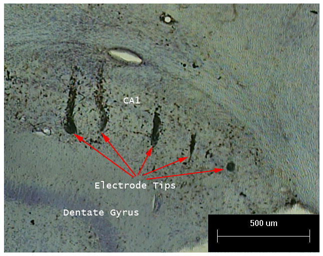
An example of electrode tip placement validation using coronal sectioned histology. Perl staining shows the tips of five electrodes in the CA1 subfield of the hippocampus. The electrode to the left terminates in the stratum lacunosum-moleculare, the middle three electrodes terminate in the stratum radiatum and the electrode to the right terminates in the CA1 pyramidal cell layer. This histological staining validated the iron content (The Perl stain highlights iron in black) and electrode track and tip locations visualized in Figure 1. Sections were then counterstained with cresyl violet to visualize cellular morphology.
2.4 Granger Causality Analysis
The microelectrode array LFP activity acquired from these electrode arrays was analyzed using GC (Granger, 1969) in order to detect and quantify directional relationships between LFP activity within bilateral hippocampal DG and CA1 subfields, during the immediate pre-seizure, seizure, and immediate post-seizure periods. The core mathematics of parametric GC methods can be found in autoregressive (AR) modeling (Chatfield, 1996). GC methods make use of the variance of prediction errors (predictions errors are ε(t), β(t), η(t), and γ(t) from AR models shown in equations(1) and (2)) to extrapolate directional relationships. For example, consider X(t) and Y(t), univariate AR models, where previous values of each time series are used to predict current value of that time series, say X from p (p is an optimized AR model order) past values of X. The coefficients bXX and bYY are the AR model coefficients.
| (1) |
The variance of the error series ε(t), Σ1, is a gauge of the prediction accuracy of the linear model of X (t). Γ1 is the analog for Y(t) time series. The next step in the calculation of GC involves the use of a bivariate autoregressive model, W(t), where the current value of each time series X(t) and Y(t) is predicted (with the same model order p) using the p past values of both the X and Y time series, shown in equation(2). Here, aXX, aYY, aXY, and aYX are the AR model coefficients.
| (2) |
The variance of the new error series is a gauge of the prediction accuracy of the new expanded predictor.
| (3) |
GC for Y to X is then calculated from the variance of the linear prediction error of X alone, Σ1, and then compared to the variance of linear prediction error of X incorporating Y, Σ2, shown in equation (4).
| (4) |
Essentially, FY→X is the ratio of the prediction error of X alone over the prediction error of X including Y. When Σ1 = Σ2 (i.e. the linear prediction error is not improved by including Y), equation (4) will yield a GC value of zero. However, when Y improves the prediction of X the log ratio is non-zero and positive a directional relationship can be inferred. The relationship in the opposite direction (X to Y) is addressed by simply reversing the roles of the two time series.
Multielectrode array LFP data from each animal was first preprocessed by down sampling to 1 kHz. The AR model order for the GC analysis was chosen to be p=25 using methodology based on Akaike's Information Criterion (AIC) and the Bayesian Information Criterion (BIC) (Akaike, 1974; Chatfield, 1996). The AIC and the BIC were both calculated, however, the BIC was used primarily due to it's correction for large numbers of parameters essentially providing tougher criteria (i.e. higher model order) than the AIC. The BIC was calculated for each model order for a given data set and plotted, yielding a plot that decreased in a pseudo exponential fashion until a steady state BIC value was reached. The point at which the steady state is reached is the model order where increases in the model order do not further improve the prediction power of the model. This was repeated for several data chunks across multiple channels and seizures suggesting model orders in the range of 15 to 20. It was then decided to round up the model order to 25 for all data to allow direct comparisons between GC results over time, provide confidence that the model order was high enough to provide reliable AR models for calculation of GC, and low enough model order to allow for reasonable computational tractability. GC was calculated using p=25 within a 1 second moving window with 50% overlap among all possible electrode pairings. Within a 1 second moving window the data was approximately stationary (Hesse et al., 2003) and long enough to provide stable AR models. This windowing technique is consistent with previous GC analysis of absence-seizure data (Sitnikova et al., 2008). This analysis produces a GC value for each directional electrode pairing and for each time window organized by source electrode, destination electrode, and time for each seizure. Thus, 32 × 32 - 32 = 992 GC directional relationships were calculated per time window (within-channel or self relationships were not investigated).
2.5 Surrogate Analysis and Post Hoc Contrasts of GC Indexes
The statistical significance of our results is estimated in two ways. First, we use a time shifted surrogate analysis where data is time shifted randomly to destroy temporal relationships within the data. This method is applied to provide a significance threshold for each individual GC value at any time point. Analysis of the time-shifted surrogate produced a threshold value of 3.66 for p < 0.01 above which the temporal relationships suggested by GC analysis can be said to be significantly different than chance for the example seizure. Practically speaking, this means electrode pairs with dark blue pixels in Figure 3 (and the supplemental movie) cannot be differentiated from random fluctuations and thus should be interpreted as having no directional relationship. The red dashed lines in the panels for figure 4 represent averaged value for the time-shifted surrogate.
Figure 3.

Example of GC analysis for a single (N=1) spontaneous temporal lobe seizure. The 1st row contains cartoon plots of the results from the GC indices calculated across all seizures (N=15) and are overlaid on MRI images of the animals hippocampus to visualize GC index directional relationships (note that the location and shape of the arrows are not meant to imply specific physiological pathways or mechanisms). GC raw results for selected time windows in the example seizure (N=1) are presented in the 2nd row. The 2nd row plots depict the strength of directional relationships among each electrode pair for all 32 electrodes by color. The electrode pairings are arranged by anatomical area. The bottom row provides the electrographic activity from the example seizure (N=1) from 4 of the 32 electrodes, one from each of the four major subfields covered by the microelectrode arrays, R-CA1, R-DG, L-CA1, and L-DG. The highlighted time segments correspond to the GC analysis excerpts shown in rows 1 & 2. These traces include one electrode among the four major hippocampal areas observed. Colors indicate the magnitude of GC results, ranging from weak (blue) to strong (red). Directional information is presented by portraying the source location on the vertical axis and response location on the horizontal axis. Starting from the lower left and moving counter clockwise, the four quadrants of each plot represent within-left hemisphere, left-to-right cross hemisphere, within-right hemisphere, and right-to-left cross hemisphere directional relationships. The first column depicts the results from prior to the behavioral onset of seizure (PS) followed by six panels representing transitions (stages S1, S2a & S2b, S3, S4, S5) in the patterns during seizure. A time shifted surrogate analysis was carried out by applying GC to the time shifted data set. This surrogate analysis yields a GC threshold value of 3.66 for p < 0.01 (dark blue in the figure), below which GC results are not significant. Note: A supplementary high-resolution animation of the GC analysis of the example seizure (N=1) presented in this figure is available on the Neuroscience Methods website.
Figure 4.
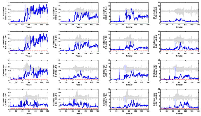
Continuous plots for the primary GC Indices for the same example seizure presented in Figure 2. Each window represents the GC Index (dark blue trace) for all of the electrode pairings from and to the areas specified on the label for each panel. For example, the top left plot (column 1, row 1) represents the GC Index or the sum of all GC results from the right DG to the L-CA1. The arrangement of the “from” and “to” areas in the subplots corresponds to the same relative arrangement in each of the GC plots shown in the 2nd row of Figure 2. For each panel, seizure data from one of the corresponding “from” electrodes used in calculation of the GC index is plotted in light grey to give a temporal context to the GC index. Additionally, significance thresholds from GC analysis of a time shifted surrogate time series is shown with a red dashed line. The seizure occurs mainly in the middle 60 seconds, the same as in the supplemental video. The GC Index is increased after seizure for 11 of the indexes, the same for 4 indexes, and decreased for 1 index. Interestingly the sole decreased index is from L-CA1 to L-DG index (column 2, row 4). This is the same index implicated for having an abnormal GC relationship observed from the L-CA1 to the L-DG prior to seizure. The spikes between 60 and 70 seconds (most prevalent in the top left and bottom right) correspond to Stage 2 cross hemisphere directional relationships.
Second, post hoc contrasts were used to better justify the qualitative partitioning of the seizure stages and the observed hierarchical evolution of temporal GC relationships during seizure onset and seizure. Pre-seizure and seizure GC temporal patterns were shown to be significantly different in a previous work (Cadotte et al., 2009), thus we examine the transition from pre-seizure into generalized seizure independently from post-generalization seizure. Due to the highly multivariate nature of the analysis, individual GC results often required averaging into GC indexes (GCI) selected by the source and destination recording locations relevant to the pattern being discussed. GCIs are averaged 1-second time windows within the corresponding stage for each individual seizure. This approach greatly simplifies the conceptual basis of the statistical analysis across the 15 seizures. Additionally, because the seizures are spontaneous and complex, the lengths of the stages vary. The average time length for each stage (N=15 seizures) is 8.4 +/- 4.4, 11.9 +/- 4.6, 11.7+/- 5.8, 6.9 +/-4.5, and 15.7 +/- 5.8 for seizures stages 1 though 5 respectively. Post hoc contrasts of GCI between seizure stages were performed using a nonparametric Friedman two-way analysis of variance with multiple comparison correction (MATLAB, friedman and multcompare functions) between GCI relative to observed qualitative patterns during seizure onset and within the seizures post generalization. For each contrast, we report the GCI used, stages compared, corresponding GCI/stage means, The Chi squared value for the Friedman ANOVA (with column degrees of freedom and total degrees of freedom), and p value for the specific contrast (post multiple comparison correction).
3. Results: Analysis of spatio-temporal dynamics
A qualitative assessment of the dynamics of GC patterns during the 15 Racine grade 5 seizure epochs suggests a consistent spatial and temporal progression of directional relationships for all analyzed seizures. To better describe this temporal progression, animations of the resultant patterns were used to define stages during each seizure based on qualitative changes in observed patterns. An example animation depicting the results from the GC analysis during one seizure is provided on the Journal of Neuroscience Methods website and is recommended as a companion to our results. This animation also includes selected electrographic signals and a summary of the patterns across 15 seizures overlaid on an MR image of the hippocampus. The temporal progression of the pattern suggests that seizure onset can be characterized by a directional relationship from the DG subfield to the CA1 subfield in the left hippocampal formation (contra lateral to the bipolar twist electrode used to create the animal model). This appearance of this directional relationship reasonably correlates with the emergence of behavioral changes associated with seizure such as blinking and chewing seen in time locked behavioral video as well as high magnitude LFP waveforms associated with seizure. For consistency, the time prior to this entrainment will be referred to as pre-ictal (PI) in this study. The subsequent time epochs are qualitatively divided into 5 different successive stages. The number of stages was based solely on the evolution of the patterns of GC relationships during these seizures (the patterns used for defining stages will be discussed later in this section) in order to better characterize and later quantify the dynamics of seizure initiation, propagation, and termination.
One of the 15 seizures was selected and displayed in parallel with its GC analysis during each stage and is depicted in Figures 3 and 4. Figure 3 depicts a colorized representation of directional relationships (middle row) organized by anatomical area (L-CA1, L-DG, R-CA1, and R-DG) during the example seizure. Electrographic time series from four of the 32 channels for the example seizure are plotted in the lower panel for visual reference. Cartoon representations of the dominant patterns from analysis of all seizures (N=15) are shown in the 1st row. Raw GC matrices for selected analysis windows are presented in the 2nd row. Figure 4 displays the GC index for the example seizure (N=1) where the magnitudes of GC indices for that seizure (calculated by summing specific directional relationships between and within observed hippocampal subfields) are displayed over time. Each of the 16 indexes presented is displayed in parallel with seizure data from one of the source electrodes used in calculation of that GC index (shown in light gray within the panels in Figure 4) to serve as a temporal reference for the GC index results for the example seizure. The following is a brief qualitative description of the 5 seizure stages suggested by the temporal patterns suggested by the GC analysis. This description will be immediately followed by a more detailed quantitative analysis where statistical significance is addressed. Neural and behavioral correlates to the stages are described where appropriate.
During the PI state there are GC relationships seen exclusively within the left CA1, as shown in Figure 3 in the PS panel. These relationships are persistent up to two minutes prior to seizure onset. Seizure onset or stage 1 is characterized by the strengthening of the relationship from the left CA1 to the left DG, illustrated in Figure 3 in the S1 panel. The spatially extent of these relationships expands in stage 2 where strong directional relationship can be seen from the left hippocampus to the right hippocampus, shown in Figure 3 in the S2a panel. Stage 2 may also include a reverberation of directional relationships from left to right and right to left, as shown by strong directional relationships from the right hippocampus to the left hippocampus in the S2b panel of Figure 3. Note that these highly directional reverberations in S2 would likely be indistinguishable from continuous global synchronization using a non-directional measure. These reverberations lessen in stage 3, contributing to the decline in total GC relationships seen in Figure 3. Furthermore, stage 3 relationships appear to be more local and less global organized. Stage 4 is a brief epoch characterized by a global increase in relationships between nearly all observed areas, as illustrated in Figure 3 in panel S4. Stage 5 patterns, where strong balanced bilateral relationships are seen from the DG to the CA1, are diametrically opposite to the directionality of the GC patterns seen in stages 1-3. This suggests that stage 4 may be a transition between stage 3 and 5. This transition is behaviorally correlated with the progression from tonic to clonic seizure behavior in the time locked video. Also of note is that relationships are primarily seen in the left hippocampus in the PI, S1, and S2 stages, but become more balanced between hemispheres in stages 3-5.
The following more detailed quantitative analysis of these results is used to validate our qualitative findings. During the PI period, relationships are confined to the CA1 of one hemisphere. Just prior to seizure onset, the strongest relationships are seen within the left CA1 (column 1, row 4, Figure 4) and between the left CA1 and left DG (column 2, row 4, Figure 4, 0-60 seconds). During stage 1 (S1) of the seizure, relationships within CA1 continue to increase (within-CA1, S1 vs. Pre, mean 5.37 vs. 2.41, Chi-sq(2,44) = 30, p < 0.02) and a new directional relationship from the CA1 to the DG (CA1 to DG, S1 vs Pre, mean 6.47 vs. 2.52, Chi-sq(2,44)=30, p < 0.02). Behavioral correlates for stage 1 represents the onset of the tonic phase of the seizure, characterized by where the animal becomes motionless. Within each animal the location (hemisphere) in which seizures appear to originate was consistent across seizures but varied by animal (5 of 6 seizures left hemisphere for rat 1, 4 of 5 right hemisphere for rat 2, and 3 of 4 seizures right hemisphere for rat 3). The relationships within the CA1 that appear to initiate the seizure cascade can often be seen up to a minute prior to the PS to S1 transition.
In stage 2, the driving influence of CA1 upon DG increased further (CA1 to DG, S2 vs. S1, mean 12.55 and 6.47, Chi-sq(2,44)=30, p < 0.02) and was accompanied by further increases within CA1 (within-CA1, S2 vs. S1, mean 10.11 and 5.37, Chi-sq(2,44)=30, p < 0.02). The relationships within the initiating hippocampal hemisphere expand to the contra-lateral (right) hippocampus (between hemisphere i.e. upper left and lower right quadrants in Figure 3, S2 vs. S1, mean 5.58 and 3.08, Chi-sq(2,44)=28.13, p < 0.05). Electrographically, stage 2 contained the first of high-magnitude waveforms commonly associated with seizure. In this example seizure, the initial directional relationship from the left hemisphere to the right (labeled S2a in the figure) was followed by a directional relationship from right to left (labeled S2b). These mono-directional cross-hemisphere relationships often reverberate between hemispheres several times and were the most striking of the features that occur during the early stages of seizure. These cross-hemisphere volleys appeared as large spikes in the GC index time series between 60 seconds and 70 seconds in the cross hemisphere GC indexes in the panels in the top left and bottom right quadrants of Figure 4.
During stage 3, the magnitude of within-hemisphere relationships declined significantly (within hemisphere i.e. upper right and lower left quadrants in Figure 3, S3 vs. S2, mean 7.40 vs. 9.77, Chi-sq(3,59) = 13.48, p < 0.11). This decrease was seen with most GC indices (shown near t=90 s in Figure 4). While the magnitudes of cross-hemisphere relationships remained elevated in stage 3 (bidirectional left and right cross-hemisphere electrode pairings, S3 vs. S2, mean 5.28 vs. 5.58, Chi-sq(3,59) = 18.44, p=0.98), these relationships were now more diffuse and became scattered among different hippocampal areas. Although the total GC index was reduced relative to stage 2 during this period (all, S3 vs. S2, mean 6.34 vs. 7.68, Chi-sq(3,59) = 17, p < 0.11), electrographically it contained the largest magnitude waveforms.
Stage 4 is correlated to the behavioral transition from tonic to clonic seizure observed in the time locked video. During this transition the animal's limbs jerk rhythmically and rapidly. This brief transition was marked by the reemergence of strong within-hemisphere relationships (within hemispheres, S4 vs. S3, mean 9.11 vs. 7.40, Chi-sq(3,59) = 13.48, P < 0.15) appearing at t=95 s as broad spikes in most of the GC indexes. However, unlike stage 2 (where high-magnitude relationships are primarily cross-hemisphere), during this epoch all observed areas were bidirectional. Moreover, the directional pattern from CA1 to DG that was observed during earlier stages is completely reversed. The primary directional relationships are now from the DG to the CA1 (from DG to CA1, S4 vs. S3, mean 10.21 vs. 7.22, Chi-sq(3,59) = 11.24, p < 0.01). At this point, the animal demonstrated rearing and falling in the time locked video consistent with Racine grade 5 seizures.
Seizure-offset or Stage 5, was characterized by a gradual emergence of low-frequency large-magnitude spike-wave events in the electrographic data. Behaviorally, the animal experienced clonic seizure until the seizure terminated. Like stage 4, the primary pattern during this stage was from DG to CA1. Although cross-hemisphere relationships are sometimes present during this final stage, these relationships declined significantly (between hemispheres, S5 vs. S4, mean 3.67 vs. 5.26, Chi-sq(3,59) = 18.44, p < 0.002). Furthermore, directional GC relationships from the DG to the CA1 that emerged during the Stage 4 transition persisted after the termination of behavioral seizure in the time locked video.
4. Discussion
The main findings of this study were that the representative cohort of spontaneous limbic seizures from an animal model of chronic TLE in our analysis follows a common spatial sequence of initiation, propagation, and termination. Two dominant patterns of LFP microelectrode array relationships were found within this sequence. The first, summarized and illustrated in Figure 3 panels PS through S2b, describe the initiation and propagation of seizure, where the seizure spreads from the CA1 to the ipsilateral DG and then the contra lateral hippocampus. If a diffuse hyperexcitable network initiates ictogenesis during this time frame, one might expect to see widespread non-directional relationships rather than a hierarchical directional progression among hippocampal subfields. The second pattern, illustrated in Figure 3 panels S3 through S4, suggests a distinct transition from an abnormal pattern (CA1 to the DG), which was observed during initiation and propagation to a more anatomically expected pattern (DG to the CA1). Interestingly, this transition occurs during the observed behavioral transition from tonic to clonic seizure. This complete reversal in the directional GC patterns may lend support to the hypothesized “resetting” of the brain during seizure (Iasemidis et al., 2004).
Overall, the detailed results of our GC and GC indices analysis suggest these methods are a reliable tool to estimate LFP directional relationships between hippocampal subfields during seizure onset and propagation. Other traditionally used methods such as power spectrum (univariate, nondirectional) and coherence (nondirectional) are not sufficient alone to capture the evolving dynamics of LFP seizure onset and spread. A summation of all GC relationships during each stage creates a nondirectional index of GC, shown in Figure 5, that is consistent with previously reported functional connectivity analysis of seizure epochs (Schiff et al., 2005). Without directionality, this type of analysis suggests that seizures are accompanied by global increases in synchronization. Additionally, the mono-directional reverberations of S2 and the global bidirectional relationships of S4 would be indistinguishable in a nondirectional analysis. However, when the directional relationships are segregated in the context of the location of the electrodes and time, our analysis suggests specific directional spatiotemporal patterns during spontaneous seizure initiation and propagation in this animal model of TLE. Furthermore, the importance in directionality in our findings is similar to specific directional findings revealed in a GC analysis of absence seizures in the thalamo-cortical region (Sitnikova et al., 2008). Additionally, GC analysis simplifies a time dependent analysis of seizure evolution due to its ability to extract the strength and direction of relationships between neural subfields from the use of only one computational method. When directly compared to other connectivity measures (Winterhalder et al., 2005), GC is shown to be among the most suitable for the monitoring of temporally dependent brain dynamics. GC is a well-established method used for examining the relationships between brain regions and is now more widely used in epilepsy (see Cadotte et al., 2009 for a more comprehensive review of effective connectivity measures in epilepsy).
Figure 5.
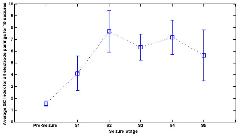
Non-directional mean (N=15 seizures) GC index of all channels pre seizure and through each of the five seizure stages. All of the directional relationships between all 32 electrodes have been averaged to produce a representation of a total nondirectional relationship. The strength of this non-directional GC index increases rapidly from the pre seizure period to Stage 1 and continues to increase until peaking during Stage 2. Following Stage 2 the non-directional index decreases during Stage 3 but briefly spikes once again in Stage 4 before terminating at the end of Stage 5. Note that this non-directional analysis shows no difference between stages 2 and 4. Overall, these results are consistent with general effective and functional connectivity assessments of synchronization during seizure found in the literature. Additionally, these results are consistent with the general dynamics observed during each of the fifteen seizures in our analysis. The average time length for each stage (N=15 seizures) is 8.4 +/- 4.4, 11.9 +/- 4.6, 11.7+/- 5.8, 6.9 +/-4.5, and 15.7 +/- 5.8 for seizures stages 1 though 5 respectively.
However, it is worth noting these results cannot preclude the involvement of unobserved brain areas outside of the hippocampus or the contribution from a diffuse epileptic network (Bertram et al., 1998; Bertram, 2009; Kudo et al., 1997; Osorio et al., 2008; Raisinghani and Faingold, 2005a, b; Sheerin et al., 2004). Unobserved time series or systems may contribute to observed functional or effective relationships. This weakness is not specific to GC analysis, however, and is shared by all methods that seek to measure the functional and effective relationships between time series. Thus, while the results presented here are compelling, they also reinforce the need for further experiments that expand the spatial coverage of electrodes to better utilize GC and other connectivity measures to characterize the mechanisms underlying seizure. For example, hypotheses for such experiments could draw upon evidence in recently published papers that suggests that the entorhinal cortex may play a strong role in seizure initiation (Amaral and Lavenex, 2007; Ang et al., 2006; Avoli et al., 2002; Barbarosie and Avoli, 1997) while activating the CA1 and DG. In Barbarosie and Avoli (1997) when the Schaffer collateral is cut in vitro (severing the anatomical linkage from the CA3 that provides modulatory input to the entorhinal cortex), epileptiform activity arises from the entorhinal cortex onto the CA1 and DG. In microlesion studies where the entorhinal cortex is damaged, similar spontaneous seizures arise in vivo (Wu and Schwarcz, 1998). Further, in vitro evidence from Ang, Carlson and Coulter (Ang et al., 2006) describe the initiation and spread of seizure-like activity from the entorhinal cortex into the CA1. These studies considered in the context of our results may suggest that time delayed influences from the entorhinal cortex may be responsible for the abnormal connectivity patterns seen in PS though S3 stages. Additionally, this may suggest that recordings from the entorhinal cortex in such an experiment may have an earlier hierarchical involvement in the analysis we present. We also hypothesize that in vivo early seizure detection studies in this rat model could be improved by using GC methods in addition to recording from strategically placed recording electrodes. Future experiments in our laboratory will include electrodes in the entorhinal cortex and the CA3 to provide a more complete representation of the involvement of the bilateral hippocampal trisynaptic circuits in spontaneous temporal lobe seizures.
In conclusion, the rat model of TLE in parallel with multichannel recordings provides a useful experimental platform from which to develop spatial and temporal analyses such as GC, a basis for further testing the hypothesis that epilepsy involves hierarchical networks. Our analysis suggests the importance in identifying and investigating directional relationships in the epileptic brain and eventually the underlying mechanisms that contribute to the transitions of patterns we observed. We postulate that the real-time detection and identification of the transitions in GC patterns across the hippocampal network during seizure onset may offer new opportunities for therapeutic intervention.
Supplementary Material
Supplemental Video: This video is a 60 second real time animated compilation of the LFP traces for the example seizure used in the text (right panel), GC results for the example seizure (top left panel), and summarized results for the GC index for all seizures (N=15, bottom left panel). For the LFP traces in the right panel, 20 seconds of data are displayed on the x-axis and 4 EEG traces from the R-DG, R-CA1, L-DG, and L-CA1 are shown. The data between the two red lines represents the data used for the GC analysis displayed in the top left panel. The top left panel displays the raw GC relationships. The source or “from” electrodes 1-32 are on the y-axis and the response or “to” electrodes are on the x-axis, and relationship magnitude is represented by the corresponding color scale. The bottom left panel is used to present summarized interactions from the qualitative and quantitative analysis of the seizure stages PS and S1 through S5. This panel and it's accompanying text changes at the transition between each stage. Note that the cartoon arrows are not meant to identify specific pathways or mechanisms they are cartoon illustrations of the GC interactions seen between electrodes embedded in these regions. Time points of note include: Time = 1 second, preictal spike with strong within L-CA1 interactions. Behavioral correlate: the animal is asleep. Notice the imbalance between hemispheres; all relationships are in the left hemisphere until S2. Time = 6 seconds, transition from PS to S1 defined as seizure onset for our analysis. Behavioral correlate: the animal awakens and displays chewing and staring consistent with tonic seizure that continues until stage 4. Time = 13 seconds, transition to S2 directional volley from the left hemisphere to the right hemisphere (labeled as S2a to correspond to Figure 2, S2a). Time = 15 seconds, volley from the right hemisphere to the left hemisphere (labeled as S2b to correspond to Figure 2, S2b), Time = 21 seconds, transition to S3. Note the diffuse lower magnitude interactions accompanied by the highest magnitude LFP waveforms of the seizure. Time = 39 seconds, transition to S4. Note the global bidirectional synchrony indicated by increases in the GC relationships for the entire top left panel. Behavioral correlate: The time locked video suggests this is the transition between tonic and clonic seizure behavior accompanied by limb shaking, rearing, and falling down associated with grade 5 Racine seizure. Time = 44 seconds, transition to S5. A new more balanced anatomically expected pattern emerges where the DG drives the CA1 for both hemispheres. Behavioral correlate includes tonic seizure that fades until behavioral seizure termination.
Acknowledgments
This research was supported by the National Institutes of Biomedical Imaging and Bioengineering (NIBIB) through Collaborative Research in Computational Neuroscience (CRCNS) Grant Numbers R01 EB004752 and EB007082, the Wilder Center of Excellence for Epilepsy Research, and the Children's Miracle Network. PRC was partially supported through the Wilder Center of Excellence for Epilepsy Research Endowment funds. WLD was partially supported through the J. Crayton Pruitt Family Endowment funds. SST was partially funded by a Fellowship Grant from the Epilepsy Foundation of America. We thank Dr. Wendy Norman and Stephen Myers for data collection and animal care, and Hector Sepulveda for MRI data collection. We thank for reviewing the behavioral videos to identify the seizure events and we also thank, Yonghong Chen, and Yan Zhang for helpful discussions. MRI data were obtained at the Advanced Magnetic Resonance Imaging and Spectroscopy Facility in the McKnight Brain Institute of the University of Florida.
Footnotes
Publisher's Disclaimer: This is a PDF file of an unedited manuscript that has been accepted for publication. As a service to our customers we are providing this early version of the manuscript. The manuscript will undergo copyediting, typesetting, and review of the resulting proof before it is published in its final citable form. Please note that during the production process errors may be discovered which could affect the content, and all legal disclaimers that apply to the journal pertain.
References
- Akaike H. A new look at the statistical model identification. IEEE Transactions on Automatic Control. 1974;19:716–23. [Google Scholar]
- Amaral D, Lavenex P. Hippocampal Neuroanatomy. In: Andersen P, Morris R, Amaral T, Bliss T, O'Keefe J, editors. The Hippocampus Book. Oxford University Press; Oxford: 2007. pp. 37–114. [Google Scholar]
- Ang CW, Carlson GC, Coulter DA. Massive and specific dysregulation of direct cortical input to the hippocampus in temporal lobe epilepsy. J Neurosci. 2006;26:11850–6. doi: 10.1523/JNEUROSCI.2354-06.2006. [DOI] [PMC free article] [PubMed] [Google Scholar]
- Avoli M, D'Antuono M, Louvel J, Köhling R, Biagini G, Pumain R, D'Arcangelo G, Tancredi V. Network and pharmacological mechanisms leading to epileptiform synchronization in the limbic system in vitro. Prog Neurobiol. 2002;68:167–207. doi: 10.1016/s0301-0082(02)00077-1. [DOI] [PubMed] [Google Scholar]
- Barbarosie M, Avoli M. CA3-Driven Hippocampal Entorhinal Loop Controls Rather than Sustains In Vitro Limbic Seizures. The Journal of Neuroscience. 1997;17:9308–14. doi: 10.1523/JNEUROSCI.17-23-09308.1997. [DOI] [PMC free article] [PubMed] [Google Scholar]
- Bertram E, Zhang D, Mangan P, Fountain N, Rempe D. Functional anatomy of limbic epilepsy: a proposal for central synchronization of a diffusely hyperexcitable network. Epilepsy Res. 1998;32(1-2):194–205. doi: 10.1016/s0920-1211(98)00051-5. [DOI] [PubMed] [Google Scholar]
- Bertram EH. Functional Anatomy of Spontaneous Seizures in a rat model of limbic epilepsy. Epilepsia. 1997;38:95–105. doi: 10.1111/j.1528-1157.1997.tb01083.x. [DOI] [PubMed] [Google Scholar]
- Bertram EH. Temporal Lobe Epilepsy: Where do seizures really begin? Epilepsy & Behavior. 2009;14:32–7. doi: 10.1016/j.yebeh.2008.09.017. [DOI] [PMC free article] [PubMed] [Google Scholar]
- Bertram EH, Cornett J. The evolution of a rat model of chronic limbic epilepsy. Brain Research. 1994;661:157–62. doi: 10.1016/0006-8993(94)91192-4. [DOI] [PubMed] [Google Scholar]
- Bollimunta A, Chen Y, Schroeder CE, Ding M. Neuronal Mechanisms of Cortical Alpha Oscillations in Awake-Behaving Macaques. The Journal of Neuroscience. 2008;28:9976–88. doi: 10.1523/JNEUROSCI.2699-08.2008. [DOI] [PMC free article] [PubMed] [Google Scholar]
- Cadotte A, Mareci TH, Demarse TB, Parekh M, Rajagovindan R, Ditto WL, Talathi S, Hwang DU, Carney PR. Temporal Lobe Epilepsy: Anatomical and Effective Connectivity. IEEE Trans on Neural Systems and Rehab Eng. 2009;17:214–23. doi: 10.1109/TNSRE.2008.2006220. [DOI] [PubMed] [Google Scholar]
- Chatfield C. The Analysis of Time Series an Introduction. 5. Chapman & Hall; Boca Raton, FL: 1996. [Google Scholar]
- Ding L, Worrell G, Lagerlund T, He B. Ictal Source Analysis: Localization and imaging of causal interations in humans. Neuroimage. 2007;34:575–86. doi: 10.1016/j.neuroimage.2006.09.042. [DOI] [PMC free article] [PubMed] [Google Scholar]
- Franaszczuk P, Bergey G. Application of the directed transfer function method to mesial and lateral onset temporal lobe seizures. Brain Topography. 1998;11:13–21. doi: 10.1023/a:1022262318579. [DOI] [PubMed] [Google Scholar]
- Franaszczuk P, Bergey G, Durka P, Eisenburg H. Time-frequency analysis using matching pursuit algorithm applied to seizures originating from the mesial temporal lobe. Electroencephalogr Clin Neurophysiol. 1998;106:513–21. doi: 10.1016/s0013-4694(98)00024-8. [DOI] [PubMed] [Google Scholar]
- Franaszczuk P, Bergey G, Kaminski M. Analysis of mesial temporal seizure onset and propogation using the directed transfer function method. Electroencephalogr Clin Neurophysiol. 1994;91:413–27. doi: 10.1016/0013-4694(94)90163-5. [DOI] [PubMed] [Google Scholar]
- Granger CWJ. Essays in Econometrics: The Collected Papers of Clive W J Granger. Cambridge University Press; Cambridge: 2001. [Google Scholar]
- Granger CWJ. Investigating Causal Relations by Econometric Models and Cross-spectral methods. Econometrica. 1969;3:424–38. [Google Scholar]
- Granger CWJ. Testing for Causlity. A personal view point. Journal of Economic Dynamics and Control. 1980;2:329–52. [Google Scholar]
- Hesse W, Moller E, Arnold M, Schack B. The use of time-variant EEG Granger causality for inspecting directed interdependencies of neural assemblies. Journal of Neuroscience Methods. 2003;124:27–44. doi: 10.1016/s0165-0270(02)00366-7. [DOI] [PubMed] [Google Scholar]
- Hill JM, Switzer RC. The regional distribution and cellular localisation of iron in the rat brain. Neuroscience. 1984;11:595–603. doi: 10.1016/0306-4522(84)90046-0. [DOI] [PubMed] [Google Scholar]
- Hoang-Minh L, Sepulveda H, Parekh M, Hadlock A, Norman W, Sanchez J, Ditto W, King M, Carney P, Liu Z, Mareci T. MRI Measurements at 17.6 Tesla in an Animal Model of Temporal Lobe Epilepsy Correlated with Histological Analysis. Epilepsia; 60th Annual Meeting of the American Epilepsy Society; San Diego, CA. 2006; 2006. p. 309. [Google Scholar]
- Iasemidis L, Shiau D, Sackellares J, Pardalos P, Prasad A. Dynamical Resetting of the Human Brain at Epileptic Seizures: Application of Nonlinear Dynamics and Global Optimization Techniques. IEEE Trans Biomed Eng. 2004;51:493–506. doi: 10.1109/TBME.2003.821013. [DOI] [PubMed] [Google Scholar]
- Kudo T, Kazuichi Y, Seino M. Effect of callosal bisection on seizure development and interhemispheric transfer effects in feline motor cortical kindling. Epilepsy Res. 1997;28:105–18. doi: 10.1016/s0920-1211(97)00032-6. [DOI] [PubMed] [Google Scholar]
- Lado FA, Moshe SL. How do seizures stop? Epilepsia. 2008;49:1–14. doi: 10.1111/j.1528-1167.2008.01669.x. [DOI] [PMC free article] [PubMed] [Google Scholar]
- Lothman EW, Bertram EH, Kapur J, Stringer JL. Recurrent spontaneous hippocampal seizures in the rat as a chronic sequela to limbic status epilepticus. Epilepsy Res. 1990;6:110–8. doi: 10.1016/0920-1211(90)90085-a. [DOI] [PubMed] [Google Scholar]
- Mormann F, Andrzejak RG, Elger C, Lehnertz K. Seizure Prediction: the long and winding road. Brain. 2007;130:314–33. doi: 10.1093/brain/awl241. [DOI] [PubMed] [Google Scholar]
- Osorio I, Frei M, Lai Y. Neuronal Synchronization and the ‘Ictio-centric’ vs the Network Theory for Ictiogenesis: Mechanistic and Therapeutic Implications for Clinical Epileptology. In: Schelter B, Timmer J, Schulze-Bonhage A, editors. Seizure Prediction in Epilepsy. Wiley-VCH; Weinheim, Germany: 2008. pp. 109–15. [Google Scholar]
- Osorio I, Frei M, Wilkinson S. Real-time automated detection and Quantitative analysis of the seizure and short-term prediction of clinical onset. Epilepsia. 1998;39:615–27. doi: 10.1111/j.1528-1157.1998.tb01430.x. [DOI] [PubMed] [Google Scholar]
- Parekh M, Hoang-Minh L, Sepulveda H, Handlock A, Norman W, Sanchez J, Ditto W, Carney P, Mareci T. Diffusion Tensor MR Imaging of the Rat Model of Mesial Temporal Lobe Epilepsy. Epilepsia; 60th Annual Meeting of the American Epilepsy Society; San Diego, CA. 2006. p. 317. [Google Scholar]
- Paxinos G. The Rat Brain in Sterotaxic Coordinates. Academic Press; Sydney, Australia: 1997. [Google Scholar]
- Quigg M, Bertram EH, Jackson T, Laws E. Volumetric Magnetic Resonance Imaging of Bilateral Hippocampal atrophy in Mesial Temporal Lobe Epilepsy. Epilepsia. 1997;38:588–94. doi: 10.1111/j.1528-1157.1997.tb01144.x. [DOI] [PubMed] [Google Scholar]
- Quigg M, Straume M, Menaker M, Bertram EH. Temporal distribution of partial seizures: Comparison of an animal model with human partial epilepsy. Annals of Neurology. 1998;43:748–55. doi: 10.1002/ana.410430609. [DOI] [PubMed] [Google Scholar]
- Racine R. Modification of seizure activity by electrical stimulation II. Motor Seizure. Electroencephalogr Clin Neurophysiol. 1972;32:281–94. doi: 10.1016/0013-4694(72)90177-0. [DOI] [PubMed] [Google Scholar]
- Raisinghani M, Faingold C. Evidence for the perirhinal cortex as a requisite component in the seizure network following seizure repetition in an inherited form of generalized clonic seizures. Brain Res. 2005a;1048:193–201. doi: 10.1016/j.brainres.2005.04.070. [DOI] [PubMed] [Google Scholar]
- Raisinghani M, Faingold C. Neurons in the amygdala play an important role in the neuronal network mediating a clonic form of audiogenic seizures both before and after audiogenic kindling. Brain Res. 2005b;1032:131–40. doi: 10.1016/j.brainres.2004.11.007. [DOI] [PubMed] [Google Scholar]
- Sanchez JC, Mareci TH, Norman WM, Principe JC, Ditto WL, Carney PR. Evolving into epilepsy: Multiscale electrophysiological analysis and imaging in an animal model. Exp Neurol. 2006;198:31–47. doi: 10.1016/j.expneurol.2005.10.031. [DOI] [PubMed] [Google Scholar]
- Schiff SJ, Sauer T, Kumar R, Weinstein SL. Neuronal spatiotemporal pattern discrimination: The dynamical evolution of seizures. NeuroImage. 2005;28:1043–55. doi: 10.1016/j.neuroimage.2005.06.059. [DOI] [PMC free article] [PubMed] [Google Scholar]
- Seth AK. Granger Causality. Scholarpedia. 2007;2:1667. [Google Scholar]
- Sheerin A, Nylen K, Zhang X, Saucier D, Corcoran M. Further evidence for a role of the anterior claustrum in epileptogenesis. Neuroscience. 2004;125:57–62. doi: 10.1016/j.neuroscience.2004.01.043. [DOI] [PubMed] [Google Scholar]
- Sitnikova E, Diaknev T, Smirnov D, Bezruchko D, van Luijtelaar G. Granger Causality: Cortico-thalamic interdependencies during absence seizures in WAG/Rij rats. Journal of Neuroscience Methods. 2008;170:245–54. doi: 10.1016/j.jneumeth.2008.01.017. [DOI] [PubMed] [Google Scholar]
- Talathi S, Hwang DU, Ditto WL, Spano ML, Mareci T, Sepulveda H, Carney PR. Circadian control of neural excitability in an animal model of temporal lobe epilepsy. Neuroscience Letters. 2009;15:145–9. doi: 10.1016/j.neulet.2009.03.057. [DOI] [PubMed] [Google Scholar]
- Talathi S, Hwang DU, Spano ML, Simonotto J, Furman M, Myers S, Winters J, Ditto WL, Carney PR. Non-parametric early seizure detection in an animal model of temporal lobe epilepsy. Journal of Neural Engineering. 2008;5:85–98. doi: 10.1088/1741-2560/5/1/009. [DOI] [PubMed] [Google Scholar]
- Wiener N. The Theory of Prediction. In: Beckenback EF, editor. Modern Mathmatics for Engineers. Chapter 8 1956. (1). [Google Scholar]
- Winterhalder M, Schelter B, Hesse W, Schwab K, Leistritz L, Klan D, Bauer R, Timmer J, Witte H. Comparison directed of linear signal processing techniques to infer interactions in multivariate neural systems. Signal Processing. 2005;85:2137–60. [Google Scholar]
- Wu H, Schwarcz R. Focal Microinjection of gamma-Acetylenic GABE into the Rat Entorhinal Cortex: Behavioral and Electroencephalographic Abnormalities and Preferential Neuron Loss in Layer III. Experimental Neurology. 1998;153:203–13. doi: 10.1006/exnr.1998.6908. [DOI] [PubMed] [Google Scholar]
Associated Data
This section collects any data citations, data availability statements, or supplementary materials included in this article.
Supplementary Materials
Supplemental Video: This video is a 60 second real time animated compilation of the LFP traces for the example seizure used in the text (right panel), GC results for the example seizure (top left panel), and summarized results for the GC index for all seizures (N=15, bottom left panel). For the LFP traces in the right panel, 20 seconds of data are displayed on the x-axis and 4 EEG traces from the R-DG, R-CA1, L-DG, and L-CA1 are shown. The data between the two red lines represents the data used for the GC analysis displayed in the top left panel. The top left panel displays the raw GC relationships. The source or “from” electrodes 1-32 are on the y-axis and the response or “to” electrodes are on the x-axis, and relationship magnitude is represented by the corresponding color scale. The bottom left panel is used to present summarized interactions from the qualitative and quantitative analysis of the seizure stages PS and S1 through S5. This panel and it's accompanying text changes at the transition between each stage. Note that the cartoon arrows are not meant to identify specific pathways or mechanisms they are cartoon illustrations of the GC interactions seen between electrodes embedded in these regions. Time points of note include: Time = 1 second, preictal spike with strong within L-CA1 interactions. Behavioral correlate: the animal is asleep. Notice the imbalance between hemispheres; all relationships are in the left hemisphere until S2. Time = 6 seconds, transition from PS to S1 defined as seizure onset for our analysis. Behavioral correlate: the animal awakens and displays chewing and staring consistent with tonic seizure that continues until stage 4. Time = 13 seconds, transition to S2 directional volley from the left hemisphere to the right hemisphere (labeled as S2a to correspond to Figure 2, S2a). Time = 15 seconds, volley from the right hemisphere to the left hemisphere (labeled as S2b to correspond to Figure 2, S2b), Time = 21 seconds, transition to S3. Note the diffuse lower magnitude interactions accompanied by the highest magnitude LFP waveforms of the seizure. Time = 39 seconds, transition to S4. Note the global bidirectional synchrony indicated by increases in the GC relationships for the entire top left panel. Behavioral correlate: The time locked video suggests this is the transition between tonic and clonic seizure behavior accompanied by limb shaking, rearing, and falling down associated with grade 5 Racine seizure. Time = 44 seconds, transition to S5. A new more balanced anatomically expected pattern emerges where the DG drives the CA1 for both hemispheres. Behavioral correlate includes tonic seizure that fades until behavioral seizure termination.