Strategies and Tactics in Multiscale Modeling of Cell-to-Organ Systems

Abstract

Modeling is essential to integrating knowledge of human physiology. Comprehensive self-consistent descriptions expressed in quantitative mathematical form define working hypotheses in testable and reproducible form, and though such models are always “wrong” in the sense of being incomplete or partly incorrect, they provide a means of understanding a system and improving that understanding. Physiological systems, and models of them, encompass different levels of complexity. The lowest levels concern gene signaling and the regulation of transcription and translation, then biophysical and biochemical events at the protein level, and extend through the levels of cells, tissues and organs all the way to descriptions of integrated systems behavior. The highest levels of organization represent the dynamically varying interactions of billions of cells. Models of such systems are necessarily simplified to minimize computation and to emphasize the key factors defining system behavior; different model forms are thus often used to represent a system in different ways. Each simplification of lower level complicated function reduces the range of accurate operability at the higher level model, reducing robustness, the ability to respond correctly to dynamic changes in conditions. When conditions change so that the complexity reduction has resulted in the solution departing from the range of validity, detecting the deviation is critical, and requires special methods to enforce adapting the model formulation to alternative reduced-form modules or decomposing the reduced-form aggregates to the more detailed lower level modules to maintain appropriate behavior. The processes of error recognition, and of mapping between different levels of model complexity and shifting the levels of complexity of models in response to changing conditions, are essential for adaptive modeling and computer simulation of large-scale systems in reasonable time.

I. Introduction

The importance of developing multiscale models for integrating our knowledge of biological systems, from microorganisms to the intact human, has been emphasized in a series of papers by Coatrieux beginning last year [1]. Physiology has been the preeminent integrating discipline, but it is the combination of engineering and physiology that is putting systems together in a quantitative fashion. Though standard textbooks tend to consider only one level of complexity at a time, modern developments in genomics, molecular biology, and physiology encourage thinking through the different levels of modeling complexity, from cell, tissue, and organs to the behavior of highly integrated systems. But the path is seldom clear, because the systems are exceedingly complex.

One idea is to represent the system complexity in terms of different scales of resolution, where scaling might be spatial or temporal or both. In this conceptual approach, we start with a set of well-defined parts of the system, which represent working hypotheses about how a portion of the overall system works. These necessarily local hypotheses are useful as thinking tools, as aids to experiment design or targets for disproof, and as components for more all-encompassing models. For each such subsystem (or module), a mathematical model is described that captures the behavior of the subsystem's inputs, outputs, and state variables. These models are most commonly sets of differential, partial differential, or difference equations, but may also incorporate switches, local operations, and convergence algorithms.

A module might represent a local approximation to the operation of a more complex model, around a specific operating point. This is normally accomplished at the risk of limiting the range of adaptability of the model.

Fig. 1 is a pictorial representation of this idea. Each small pyramid represents a subsystem module. An aggregate model can be constructed from a set of such modules, and that aggregate model may itself be one of several modules at the next level of complexity. One challenge in this aggregation process is matching module inputs, outputs and state variables. A second issue is the extrapolation for “missing” modules (where a model is not known, or simplifying assumptions are made). For example, if the levels in Fig. 1 correspond to time scaling, then some of the “missing” modules might be represented as constants (over intervals of interest) at a slower time scale modeling level, such as by linearization. The level of detail that is possible (i.e., the number of modules that can be constructed) is, of course, dependent upon the availability of data on which to base the modeling.

Fig. 1.

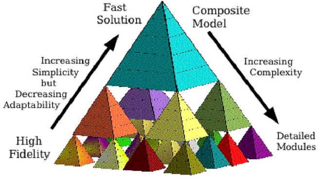
Diagram of multiscale cell model. Pyramids at each level of complexity represent individual subsystem modules.

Constructing a fully developed multiscale model is a brute force task. The level of model resolution is tightly coupled to the computational load. The high-resolution model is necessarily computationally slow. If models are to be used both as “mind expanders” in exploring systems behavior and as data analysis tools, it is critical “to compute at the speed of thought” (a misquote of the book title by Gates [2]). There is a tradeoff between the computational complexity of the model and accuracy at the cost of omitting or approximating some of the elements, maintaining the correct behavior of the model within a range of interest.

Consider the requirements to compute model solutions in real time—for example, for patient care in a clinical intensive care unit or to control the delivery of an anesthetic agent during an operation. Computational speed and accuracy are both required. While data are being acquired continuously, the high level (most aggregated) model is used in the analysis of those data. If the patient's status changes such that the reduced model form incorporated into the aggregated model is no longer within its limited range of validity, then the model resolution will need to be increased, at least for a short time. That is, more detailed modules must be used (at a higher computational cost) to capture these changes.

An overall systems approach to developing a multiscale model of physiological systems might be summarized in six steps.

Preprocessing

1. Define the model (at its highest level of resolution) and validate it against diverse data sets. This involves describing the system (as a set of interconnected subsystems), expressing the system models mathematically, writing and verifying the computer code, and then validating the modules and the system model against high-quality data.

2. Design reduced-form modules and parameterize them to match full module behavior. These reduced form models (and associated software modules) are designed to compute faster, yet to capture the varied essences of the fully developed models, parameterizing them for specific conditions by optimizing their behavior against the fully developed equivalent modules or elements.

3. Determine ranges over which the reduced-form modules are valid.

Processing

1. Monitor variables for deviations from expected or valid behavior. When appropriate, replace inadequate modules with more detailed, lower level modules.

2. Replace lower level modules with aggregated, higher level modules, thereby returning to a state requiring less computation, when conditions allow, i.e., when within the range of conditions for which a reduced-form model has been demonstrated valid.

Postprocessing

1. Validate performance of the multiscale model simulation against expectations and against experimental or clinical data.

Steps 4 and 5 involve the adaptation of the simulation to changing conditions, in order to attain and maintain both accuracy and efficient computation. When reduced-form models become less valid in representing the physiology, the computation must shift to use either the full subsidiary model or an alternative form of the reduced model (in either case using automated reconfiguration of the model). Detection may involve empirical recognition of signal features, because either an artificial intelligence approach or a signal detection technique may be used. Given that sets of reduced modules are available, successful automation of steps 4 and 5 permits the full model to go through successive reductions, decomposition as conditions demand, and reduction again.

In this paper, we discuss the variety of mechanisms for maintaining the accuracy of computationally fast composite models, while dynamically changing to the slower, more complex middle and lower level modules. This approach to carrying out simulations, with continuous monitoring and dynamic control of the computing carried out at subsidiary modules in a multiscale model system, is analogous to changing numerical methods over time as the degrees of stiffness vary.

Unlike simulations in engineering and physical sciences, in physiology the processes are often unknown and are being redefined. However, in both life sciences and physical sciences, a common principal goal is to determine integrative behavior. Error in multicomponent physiological modeling is potentially large because almost every module provides inputs to other modules, propagating any error. In our adaptive approach the idea is to control the processes of simulation to detect error and to adjust the computation to avoid it. This is a work in progress, and many advances are needed to refine the methods.

II. Multiscale Modeling of Cardiac Performance: Modeling Cell-to-Organ Systems

Modeling of the physiome from genome to integrated organism is currently impossible: there is not enough information available, particularly at both the lowest and highest levels, and there is not enough computer power to compute what is known at the intermediate levels even if one actually succeeds in putting it into one model of human physiology. For example, the three levels in Fig. 1 might represent the cell, from the biophysical/biochemical level of proteins at the bottom, to subcellular modules for processes like metabolism, energy generation, contraction, etc., in the middle level, to the top level of integrated cell behavior. Below the bottom level would lie the levels of gene regulatory networks and of transcription and translation. Above the composite model cell level are the levels of tissue, of organs, and of organ systems and their regulation.

While the fully developed lower level biophysical models can be designed to account for the function of a particular protein over a wide range of conditions, changes of temperature, pH, ionic milieu, phosphorylation, and so on, much of this adaptive condition of the behavior must be sacrificed at the higher levels in order to keep the larger, midlevel models running “at the speed of thought” or at least at a speed compatible with use in optimized fitting of models to data.

Cardiac electrophysiology has been a target for model reduction strategies. A cardiac cellular action potential model requires accounting for many ionic currents, ionic buffering, and ion pumps and exchangers for maintenance of the intracellular milieu, about 120 equations in the model of Michailova and McCulloch [3]. Even so, a pair of equations from Fitzhugh [4] and Nagumo [5] can represent the propagation of excitation through the myocardium very well, a huge reduction in computation time. Poole et al. [6] looked upon such reductionist approaches in a broader way, comparing the ordinary and partial differential equation models with cellular automata models.

That computation time is a problem is understandable in view of the complexity inherent to the biology. The route from gene to function is anything but clear, and in fact there is usually no cause-and-effect chain of understanding between gene and phenotype. Not only is the idea “one gene—one protein” [7] now replaced by the recognition that in humans one gene may contribute to perhaps 10 proteins, but, lacking intermediate level information to define cause-and-effect relationships, one looks for statistical evidence that a particular gene is associated with a particular phenotype. At the protein level, an amino acid substitution in an enzyme or channel protein may dramatically alter its function. At the level of integrated cellular biochemical systems, models must be expressed in dynamical equations in order to capture the nuances in rate expressions and the thermodynamics of reversible reactions. Matrix calculations that account only for steady-state relationships cannot represent system changes over time. For assurance of validity, the models must also capture conservation conditions such as balances of mass (including the solute mass bound to enzymes), energy, and constituent fluxes. Tissue-level models are composed of such cellular models with appropriate anatomic measures of volumes and distances. As an example, reduced forms are in use for steady-state tracer analysis of images from positron emission tomography (PET) and magnetic resonance imaging (MRI). Physiological modeling, however, requires handling transients in response to external changes, or tracer transients in chemical steady states, situations in which steady-state fluxes do not provide the answer.

Some lessons have been learned in the applications of transport modeling to the interpretation of image sequences from PET and MRI. Models of cell-to-blood solute exchanges and chemical reactions must be simplified to be computed fast enough to aid in the repetitive trial-and-error method of devising hypotheses and designing critical experiments. Eliciting physiological parameters from the data sets acquired over minutes to hours involves fitting time-domain solutions iteratively for each region of interest (ROI), often for hundreds of ROIs in order to create a parametric image conveying physiological information about the tissues. To save time, reduced-form models must be parameterized to reproduce the response functions of the full model, for any given element or module, an optimization that results in a descriptor that is correct over only a limited range of model validity. Error correction requires resorting to the more complex and detailed forms of the modules and elements. The process of recognition, going down the hierarchy of model forms and back up is difficult, prone to error, and time consuming, but is essential for modeling large-scale systems in reasonable time.

The physiological response to exercise illustrates a point, namely, that there is rather tight regulation of blood pressure in spite of large changes in body metabolism, cardiac output, and vascular resistance. In general, in the adult, there is a nested hierarchical control, the lowest levels relating to the regulation of transcription and the generation and degradation of proteins. Currently, computational models integrating cellular events into tissue and organ behavior utilize simplifications of the basic biophysical and biochemical models in order to reduce the complexity to practical computable levels. The “eternal cell” model [8], [9], focused as it is on cellular ion and substrate and energy regulation, is relatively simple but still complex enough that it has reduced forms for specific applications. Reductions compromise the adaptability of the models to respond correctly to dynamic changes in external inputs, for these normally require adjustments in rates at the biophysical, biochemical, and gene regulatory levels.

The cardiac responses to exercise involve cardiac cellular energetics, contractile force development, beat-to-beat ejection of blood from the cardiac chamber, the regulation of blood pressure and cardiac output, and its redistribution throughout the body. The five levels of modeling we consider in a cardiovascular system model are these:

• protein kinetics (for individual channels, transporters, exchangers, receptors, and enzymes);

• cellular subsets or reaction groups (glucose or fatty acid metabolism, oxidative phosphorylation, contraction, cellular excitation);

• integrated cell systems, our “eternal cell” (metabolic rate, ionic balance, redox state, pH regulation);

• multicellular tissue-to-organ function (endothelial, smooth muscle, and parenchymal cell interactions and intercommunication, contraction of heart, pressure generation).

• physiological system function and regulation such as heart rate and blood pressure.

Our specific exemplary cardiorespiratory systems model is a five-level model with severely reduced representation at the supporting levels and is limited to a high-level representation, yet it gives appropriate pressures and flows in the circulatory and respiratory systems, gas exchange including oxygen and carbon dioxide and their binding to hemoglobin, bicarbonate buffering in the blood, H⁺ production in the tissues, control of the respiratory quotient (RQ), baroreceptor and chemoreceptor feedback control of heart rate, respiratory rate, and peripheral resistance. This is a large-scale model that summarizes the information from key studies done over the past century and that adapts to changing conditions in a limited way. It is available now for public use as the model VS001¹ and serves as a basis not merely for the understanding of physiology, but for pathophysiological processes and their consequences. With development, it will be a good framework for pharmacokinetics and pharmacodynamics, as the tissue processes become broadly enough described to handle blood–tissue transcapillary exchange and cellular metabolism.

A cell model needs to be linked with an overall circulatory system model in order to support variation in tissue events (varying blood flows, metabolite production, substrate exchanges). While this can be done at a fairly simple level for handling a few solutes at a time, as we have done using axially distributed capillary-tissue exchange models accounting for gradients along capillaries [10], [11], these models are themselves computationally demanding when used in their fully expanded forms accounting for intraorgan flow heterogeneity [12] and for exchange, metabolism, and binding in red blood cells, plasma, endothelial cells, interstitium, and the organ's parenchymal cells, and require up to the equivalent of 80 000 differential equations. These particular model types [blood–tissue exchange (BTEX)] [11] are designed so that parts not used are not computed, saving much time, and they can be reduced to the form of a single-compartment, lumped model.

Control of contractile performance is defined by influences external to the cardiomyocyte, namely, levels of sympathetic and parasympathetic stimulation and circulating hormones, and cardiac filling pressures (preload), the arterial pressure against which the heart ejects blood (afterload), the heart rate, and the peripheral vascular resistances. Integration of these events into a whole organ model accounting for regional heterogeneities in flow [13], [14] and contractile stress [15], [16] gives rise to a level 4 organ model with spatial patterns of regional flows and oxygen consumption that are fractals in space but are stable over time. When put into the context of a fully developed three-dimensional finite element heart model with all the correct fiber and sheet directions, one should be able to discern whether or not the spatial heterogeneity of local flows is governed by the local needs for energy for contractile force development. It takes such a fully developed model to examine the simple hypothesis that local muscular work loads determine local blood flows, so this hypothesis has yet to undergo testing.

Literally hundreds of published models, some in texts [17]–[20], serve as background to our efforts in composing a five-level model with full sets of equations. At the cardiorespiratory system level, the classic model of Guyton et al. [21] was the pioneer. Of the many recent models near that level, there are several by Clark et al. [22] illustrating a coherent and extensive body of work. Reproducible models, carefully documented, and published with full sets of equations, parameters, and initial conditions, are remarkably rare, but include Hodgkin and Huxley [23], Beeler and Reuter [24], Winslow et al. [25]–[27], Noble [28], Sedaghat [29], and [30], some of which can be found at our Web site,² along with many subcellular level, transport, and electrophysiological models.

Tissue-level models are composed of a set of cell models (myocyte, smooth muscle cell, endothelial cell) all interacting in governing and in being influenced by interstitial fluid (ISF) concentrations. For example, in hypoxia, where ATP is released from myocytes, the extracellular hydrolysis of ATP to AMP is due to the interstitial alkaline phosphatase, which is abundant at the arteriolar end of capillaries, not the venous end. This localization requires using axially distributed models [11], [12], [31]–[36] for representation of the convection–diffusion–reaction events.

Cell-to-organ models will be vehicles for integration from observations of many sorts, mRNA array sequences, gas chromatography/mass spectrometry metabolomic arrays and capillary electrophoresis/mass spectrometry proteomic arrays, nuclear magnetic resonance spectroscopy and optical observations of cellular kinetics, electrophysiology, ion regulation, and so on. While the “eternal cell” lacks the key ingredients for gene regulation, it is centrally positioned to be augmented by data and synthetic models of signaling networks and to define the effects of specific genetic variants, as in the studies by Saucerman, McCulloch et al. [37], [38]. Signaling networks (i.e., ligand-receptor binding, GTPase activation, intracellular phosphorylations) and genetic regulatory networks (gene transcription initiation, activation, repression, etc.) have been extensively studied in recent years and will be incorporated. Palsson and colleagues [39], [40] have developed interesting approaches to signaling and regulatory networks using a constraint-based steady state. For cardiac studies we think there is an ideal preparation for studying the regulation of transcription of contractile proteins, namely, the chronically paced heart of ambulatory dogs, in which hypertrophy, up-regulation of myofilament proteins, develops in late-activated regions with increased workloads, and in which atrophy occurs in early-activated regions of diminished work [41], evidence of down-regulation of synthesis of the same proteins. The “eternal cell” model, by providing a basic energetically and metabolically based picture, is considered a key step to augmenting the powers of genomic and molecular biology. It is also a key to determining how genetic and cellular interventions can affect the physiology of the whole body.

For each component subsystem in a cardiovascular/respiratory model, one or several reduced models are to be developed; these may use differing levels of approximation or may be specific for use in different ranges of model functions, as in metabolism at rest versus exercise. Over a five-level hierarchical system, one must use successive levels of reduction, coalescing each time a few lower level modules into a computationally more efficient composite model. However, each up-the-scale reduction limits the range of operational validity of the composite model.

III. Verification and Validation

The verification, by testing to make sure that the computation provides results correctly from the equations, of such models is difficult because there are often no analytical solutions with which to make comparisons. The assurance of correctness of the code starts with writing the equations to provide internal checks for unitary balance, providing units for all parameters and variables and using a compiler or code checker that checks every equation, as is done in the JSim simulation system.³ We strongly advocate incorporating unit balance checking in every simulation system. The second step is to write into the particular program the equations checking for balances of mass, charge, momentum, energy, etc. For biochemical systems, there should be checks for the masses of particular components, H⁺ ion, NAD/NADH, total phosphate, carbon and nitrogen and sulfur, and any other moieties that are thought to be conserved while existing in multiple forms. Water, osmotic, and ionic balances are essential, but are not easy to impose as constraints on the system.

Initial standard approaches to checking numerical stability are to use different time step lengths and several different solvers while testing with a wide range of parameter values to cause different degrees of stiffness. In some cases, it is possible to test steady-state behavior in limiting cases and to determine agreement with known analytical results or simplified solutions. Such procedures do not guarantee, but help to ensure, the correctness of the mathematical model (irrespective of its validity regarding experimental data), computational algorithms, and computer code.

The validation, by comparison of model solutions with experimental data, that the model is a reasonable representation of the biology with its physicochemical, anatomical, and mass constraints, is the scientific core of any model-based project. Without it the modeling would be an exercise in defining a concept. True “validation” requires testing the model, component-by-component and level-by-level, through to the integrated systems level, against high-quality carefully chosen data. Many of these data sets will have already been selected implicitly, for each of the basic biophysical modules would have been validated on particular experimental data; this raises overtly the question of whether or not the module's form or its parameters are appropriate for the conditions under which the aggregated model is operating. Obtaining the original data sets is difficult and often requires asking the original authors for their data. This often fails because the data have not been retained. We really need an international repository of experimental data, and need to strengthen the resolve of journal editors and granting agencies to push for the archiving of experimental data and descriptions of experimental and analytical methods.

In physiology and pharmacology the digitized data are often of time course responses to stimuli such as changes in concentrations, pH, tracer addition, oxygen deprivation, and so on. Other validation data are observations of enzyme levels, metabolite concentrations, anatomic measures, and tissue composition. Fully detailed metabolic profiling, providing data during transients, are needed and await technical developments in the field. Using constrained mass, density and volume considerations [42] powerfully resolves multiple observations into a self-consistent mass-conservative context for biochemical systems analysis.

For validation a dynamic model solution is fitted to the data using a priori constraints wherever possible from the anatomy and the thermodynamics. A model is considered a viable “working hypothesis” when the model fit is good for a variegated set of observations, preferably from several different laboratories. Examples of validated models can be found in [11], [43], [44].

The validation of reduced-form models has to take into account that there may be more than one of them. Each model will be an approximate analog to the full-complexity parent model over a different limited range of conditions and parameter settings, and therefore each version has to be validated. These different forms can either be completely different mathematical equations or different sets of parameter values. The validation therefore requires several steps: namely, validation of the full-complexity model, definition of the range of conditions over which the approximation is valid, and reaffirming the validation against experimental data, seeking data over wide ranges of experimental or physiological conditions

IV. Constructing Reduced-Form Models

Cellular models are good targets for testing how best to construct reduced models, since fully detailed cell models are currently being developed. A reduced model should use physically meaningful quantities under the constraint that the reduced model forms are descriptive of the behavior of the full models within a defined margin of error over a prescribed range of conditions. Each is an approximate representation that improves computational efficiency, but sacrifices some accuracy in being applicable only over a restricted set of conditions.

Reducing a complex chemical reaction system into a simplified kinetic model has a long history in chemical dynamics, a subfield of chemical physics [45]. One standard approach is to reduce a kinetic model by its time scales. With a given time scale as the objective, there will be fast time scales on which all the kinetics are treated as quasi-steady state, and slow time scales on which the dynamic variables are considered constant. This is formally known as singular perturbation in applied mathematics [46], [47]. Well-known examples of such are the studies on the Belousov–Zhabotinsky reaction (oregonator) and the Hodgkin–Huxley theory (FitzHugh–Nagumo) [48]. In the latter example, the two-equation FitzHugh–Nagumo model replaces the four-equation Hodgkin–Huxley model, so enhancing efficiencies in computing the spread of excitation in a three-dimensional domain. The advantage of this approach is that the reduced model usually preserves a high level of connection with the original mechanistic model; hence, the model parameters are physically meaningful. The drawback is that this is a task for trained specialists.

Approaches to reduced model derivation usually involve reductions in the kinetics of the model. Essentially all the computational cellular biology models that are based on nonlinear chemical kinetics involve enzymes. The extensive literature on model reduction in enzyme kinetics reflects the difficulty of multiscale model reduction as well as the central role of enzyme kinetics in computational biology. A careful biochemical analysis of enzyme catalysis or channel or ion pump function usually leads to a detailed mechanistic scheme with multiple steps and multiple intermediate conformational states (species). While molecular biochemists strive for more complete description of the details, not all the details are important to the description of the dynamics and physiological functions. Recognizing that it is impractical to compute large networks of protein reactions at the level of either detailed molecular motions or of the kinetics of all the conformational states, model reduction is useful to move from biophysical- to cellular-level integration. The key to faithfully modeling physiological function through model reduction is to know which aspects of the model require preservation at higher levels and which aspects can be relatively crudely approximated without compromising the robustness of the system [49].

V. Adaptive Multiscale Modeling

For the multiscale modeling and simulation of complex biomedical systems, it is necessary to represent the system, either mathematically or in computer code, with verifiable accuracy. This must be done for all subsystems (or modules), at each level of scale. The multiple scales of interest can be spatial, temporal, or both, and might involve different scaling variables.

One goal of such a multiscale model representation is to gain computational efficiency during real-time simulation of the system, especially if control actions are taken on the basis of model predictions. The reduced-form models must accurately match the behavior of the full models (for the components of interest, at that level) over a prescribed range of conditions. They must be computationally more efficient than the full model. It is important that they interact correctly with other components at the same level and allow for correct incorporation into the next higher level models, with the goal being to attain accurate simulations of the desired behavior, while minimizing computation.

In recent years, the mathematics of multiscale systems modeling has been of great multidisciplinary interest. Three excellent documents that address this issue are the results of workshops sponsored by the U.S. Department of Energy in 2004 [50]–[52]. In particular, [51] contains a collection of representative references regarding algorithmic approaches, and applications to different fields. The range of types of multiscale modeling applications is quite broad, ranging from ecological model aggregation [53] to representations of materials properties at the nanoscale.

As might be expected given the diversity of types of multiscale systems, different types of applications have special features which will limit generality of a single approach toward multiscale modeling. Of particular interest to the authors is the development of well-described and implementable procedures based upon constrained system identification methods, to adaptively switch among models of varying complexity, during real-time simulation.

Systems identification methods (using input/output representations) are a common choice for fitting biological models to the measured data. Most often, a discrete time representation of the system is used, corresponding to time-sampled continuous time signals. A wide variety of system identification algorithms (mostly based upon recursive least-squares methods) are available and well understood for such systems. From a given set of system input–output data, different order models can be fit, with quantifiable accuracy for each. “Artificial data” obtained from computer simulation of detailed, complex models can also be used, to supplement (or in place of) measured input–output data.

Two key questions that must be addressed are:

• how to insure that identified model parameters are sensible, and do not violate known-to-be true relationships among system variables;

• how to switch back and forth between levels of complexity during real-time simulation.

The proposed solution to both of these problems is through the imposition of equality and inequality constraints on identified model parameters.

To illustrate aspects of this adaptive switching problem, we consider here a well-known class of models (dynamic system models that are linear-in-parameters) which, nonetheless, are sufficiently complex that key issues of interest arise. This choice of model class is for pedagogical reasons (and because it is the easiest case to consider), but we believe that the proposed approach has greater applicability (although not yet developed).

Dynamic system models that are linear-in-parameters are well established as a useful class of models for system identification and adaptive control. This class of models allows for linear systems, and also for a large class of nonlinear systems that can be represented as time series expansions in the input and output variables.

Models under discussion have the following form (at each level of complexity, and for each subsystem at the same level):

$$y(t)={\varphi }^T(t‐1)\theta$$

where y is a vector of observed output variables at time t. There are n unknown parameters θ. The vector ϕ of regression variables (or regressors) contains the data (i.e., the measured values of system inputs and past outputs or functions of them) which are used, for each time t, to fit the parameter estimates θ. The values of n and the parameters θ are generally different for each module at the same level of complexity and tend to increase as the level of model complexity increases.

Any text with “systems identification” in the title will provide the reader with a detailed description of these methods to estimate the model parameters (for a single module) [54]. The use of weighted recursive methods allows for capture of time-varying parameter changes in fitting biological systems. An example of the application of these methods to a physiological system is the identification of models of electrically stimulated muscle in paraplegics [55].

There are several issues that must be addressed in applying parameter identification algorithms for any single model (of a particular level of complexity). Among these are: 1) excitation issues and problems related to fitting parameters of closed-loop systems; 2) offset identification; 3) the identification of input–output delays (i.e., latencies); 4) model order selection; and 5) the imposition of known constraints in parameter identification. These are described in the remainder of this section. Additional issues concerning multiscale model fitting are described in Section VI.

A. Excitation Issues and Problems Related to Fitting Parameters of Closed-Loop Systems

In order to identify the parameters, it is required that the system input signal (that is, the time series of inputs) vary sufficiently to “sufficiently excite” the system, so that all of the parameters that we seek to identify are contributing to the resulting output signal. This is analogous to needing to vibrate all of the strings of a violin to model the response of the instrument to fingers and bow. For this reason, an approximation of white noise (generated by a pseudorandom binary sequence) is often used as a test input when identifying the parameters of a linear time invariant system, since the spectrum of this signal has a wide range of frequency content.

When identifying a system that is under closed-loop control, it may not be possible to have the required excitation for good parameter identification. If it is desired to maintain a constant output level, and the control system is working effectively, the resulting input may be almost constant, providing little or no parametric information. This is a complicating factor when fitting parameters to the subsystems of a physiological system during its operation. One strategy to address this problem is, when possible, to collect data from the subsystem of interest when it is somehow isolated or decoupled from interconnecting subsystems—so that external control loops are not in operation. Of course, the resulting subsystem performance may not be normal in such an unusual situation, which may lead to incorrect model parameters. Another approach is to deliberately add a small disturbance input signal, thereby ensuring adequate excitation for purposes of model parameter identification.

B. Offset Identification

In many biological systems, there is a nonzero output value, in response to zero input. That is, the system may have an offset. When using a parameter identification like weighted recursive least squares, the consequences of an offset change on the estimated parameters can be significant.

Consider the situation shown in Fig. 2, in which the steady-state input–output gain of the system is computed from parameters that are identified using a weighted recursive least-squares algorithm. The squares represent measured data points. The original offset value, the ordinate intercept [1], leads to the estimated gain shown by the slope of line 1. At some time, the offset changes to value [2], resulting in a new input–output relationship shown by line 2. It has the same gain as line 1, since only the offset value has changed. New measured data points are shown by round dots. Unfortunately, the recursive algorithm will fit line 3 to a combination of these new and old data points. The resulting estimated gain has the wrong sign—which could be catastrophic if this gain were being used, for example, by an adaptive controller. Any stable feedback system would be made unstable by such an identification error.

Fig. 2.

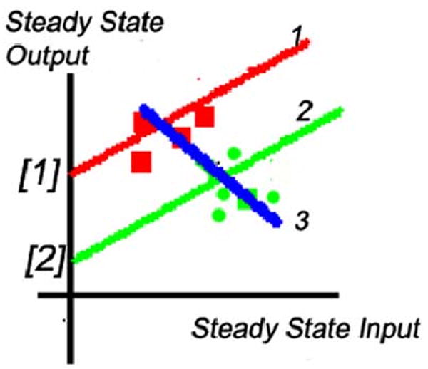
Effect of change of offset on estimation of system steady-state gain. Measured data points are indicated by the small squares.

To avoid this type of problem, it is possible to identify the offset value directly as an additional parameter in the θ vector. This is often difficult to do, because the offset may change frequently, and thus obtaining data that is sufficiently exciting for identification may be impossible. A more effective way to handle offset identification is to filter the input and output signals, to separate low-frequency and high-frequency effects. The low-frequency effects can be used to estimate the offset, and then (after adjusting the data for this estimate offset), the high-frequency effects can be used to identify the remaining model parameters. This idea was developed for, and applied as part of, the adaptive control of cardiac output using a closed-loop drug infusion system [56].

C. The Identification of Input–Output Delays

Many biological systems have input–output time delay. The magnitudes of such latencies are additional model parameters that must be identified. In some cases, they are time varying (such as physiological responses to drugs, as receptor sites are filled). Fixed delays in the response of the system can be modeled in the above representation by shifting the indexes of the input-related terms in the regressor vector by the amount of the delay. When the delay is unknown, an alternative is to determine it by looking for the parameter related to the earliest input signal where the identified value is not “close” to zero. A variant of this method has been applied, as a part of an adaptive controller of blood pressure in response to sodium nitroprusside infusion [57].

D. Model Order Selection

In practice, the order of the model, as denoted by the number of parameters, n in the previous discussion, and hence the dimension of the regression vector ϕ, are often not known in advance. While consideration of model order is usually associated with statistical time series analysis where “order” implies the number of elements needed, e.g., for autoregressive moving average (ARMA) characterization, the same ideas can be applied to deterministic modeling where there are multiple levels of detail that might be used or not, depending on the accuracy required. One way to select the best choice of model order is to compare the performance of a set of models, each using different values. But the larger the number of parameters in the model, the better it will fit any given set of data. The key issue is which order model will be best when then tested on a new set of data (other than the data used to fit the model).

For linear-in-parameter models, the set of models (of different order) that are involved in this determination might be fit using the recursive least-squares identification methods for various choices of n. A more computationally efficient approach is to use ladder time model structures, where each model of a given order p contains the first p parameters of higher order models. This facilitates the use of order recursive identification algorithms, the most common of which are based on the Levinson–Durbin recursion. In particular, order recursive identification can be used in real time, to adjust model order, increasing or decreasing it as appropriate to best fit measured input–output data. Several methods have been proposed to select model order for this class of system. The three most popular are the Akaike Information Criterion [58], the Final Prediction Error [59], and the Minimum Description Length [60] methods.

E. Imposition of Known Constraints in Identification

When fitting parameters for the model of a physiological system, constraints on the allowable values of parameters of functions of the parameters are often known. Further, a particular value may be nonnegative or greater than a known threshold. The system gain might lie between two values. A linear model's poles may be stable. The information contained in inequality constraints on allowable parameter values should ideally be used in the parameter identification process.

In complex interconnected systems like the circulatory and respiratory systems or large biochemical networks, there are many fewer degrees of freedom than there are equations and parameters. As a result, there will arise equality constraints on model parameters. These can also result from interactions between subsystem levels.

When such constraints on the allowable values of identified parameters are based on “known to be true” facts, this information can be exploited to improve model fitting. For example, known facts about the shape of a particular non-linearity (the “muscle recruitment curve”) were used, as an equality constraint on the parameters, in the simultaneous real-time system identification of nonlinear recruitment and muscle dynamic properties in the quadriceps muscle of spinal cord injury subjects [61]. Methods for imposing inequality constraints, based upon a combination of linear programming methods combined with least-squares methods, have been applied to the adaptive control of drug infusion for regulation of cardiovascular system variables [62].

F. Other Relevant Model Types

The five issues described above are relevant to many other classes of models, beyond linear-in-parameter models. Physiological subsystem models need not take the form of difference or differential equations, with parameters and variables taking real number values. For example, at the molecular level, a dynamic algebraic system representation can be used for the prediction of local variations of DNA helical parameters, with the base pair sequence (from one end of the helix to the other) considered as the system input signal, and geometric features of the DNA molecule (at each location along the helix) considered as the output. Parameter identification methods have been applied to this type of system, using genetic algorithms [63].

Some systems essentially switch between different models, based upon discrete events or certain variables traveling across switching boundaries. This type of system is challenging to represent, because such transitions are generally not fully deterministic. One approach to capturing the behavior of systems of this type is to represent them as switching between different models, due to an underlying Markov process. The stochastic control theory for such “jump systems” is well developed [64]–[69] but the design of parameter identification methods for such systems is an open question.

Models need not be numerical. For example, they might be composed of logical (“if–then”) rules. Such rules might be handcrafted, but they can also be extracted from sets of input–output data using a variety of methods, including artificial neural nets and other artificial intelligence methods. For example, a set of rules using foot force sensor information for real-time gait event detection in spinal cord injury patients during paraplegic walking has been extracted using fuzzy system identification [70], [71], which enables decision control based upon observations.

VI. Adaptive Model Modification

Five different actions are involved in adaptive model modification: 1) reduction: switching to a reduced-complexity model (also called compression or aggregation); 2) model switching: substituting one reduced-complexity model for another when conditions change or inadequacies are detected; 3) reparameterization: abruptly or gradually changing a model's parameters to make it more accurate under current operating conditions; or 4) decompression: using a higher complexity model to obtain more precise results and also possibly to recalibrate reduced form models (also called decomposition, disaggregation, and lifting); and 5) detecting when to switch between models. Each of these is briefly described below, and then methods for determining when to take these actions are addressed.

Determining when to execute these model modifications is based upon real-time monitoring of the accuracy and effectiveness of the simulation currently in use (i.e., its level of complexity and the modules involved). The decisions to take any of the five types of actions listed above might involve error signal analysis (discussed in greater detail below), or it might involve rule-based methods.

A. Reduction/Aggregation/Decreasing Resolution

For each component subsystem, at each of the levels of the five-level model, there may be several reduced-order models fit from observed inputs and outputs to the component subsystem. These families of identified models will generally be nested, and of increasingly complexity. Aggregation involves combining modules at a level into a single module at the next level of simplicity. One approach to doing this is to solve an embedded optimization model—finding best approximate fit of a simplified model solution to that of the more complex parent model using a least-squares minimization of some particular objective function. An alternative approach, when decreasing resolution for a single module from a more detailed level, involves lattice form representations, where first n parameters of nth order and (n + 1)th order models are the same. Note that the term “aggregation” is sometimes used to refer to combining models, without changing the complexity of the modules.

Reduction may be appropriate when higher resolution models are not needed to obtain the desired level of accuracy, when they will cost too much in computational load, or when there are mismatches between modules due to lack of data. Reduction can be thought of as the implementation of Occam's Razor, with rationality in terms of first principles.

B. Model Switching

Substituting one reduced form model for another is useful when prior exploration has defined ranges within which different model variants are applicable. Then it is a simple decision to switch to a different model variant when the system variables being computed cross a defined limit. An important requirement for smoothness in the transition is that the two variants should have very similar behavior in the neighborhood of the defined limit.

C. Reparameterization

Changing the parameters of a reduced-complexity model to make it more accurate under current operating conditions is often problematic. As described above, in parameter identification algorithms, a “weighting factor” can be chosen that allows the model parameters to track slowly varying system changes (by discounting past input and output data, relative to newer information). This use of weightings in the identification algorithms allows the identified reduced-complexity models to be adaptively fit to changing conditions.

In “black box” models, the identified parameters of the model may not have intuitive physical meaning. Often “obvious” facts about the system, which can be expressed as constraints on the allowable values of identified parameters, may even be contradicted by the identified parameters of the model. This problem can be reduced when, under certain conditions, a priori information about the system can be used in the system identification process to obtain parameter estimates that are more realistic and meaningful than if this knowledge is ignored.

As mentioned previously, this can be done through the imposition of inequality or equality constraints on the identified parameters. For example, a constraint might be imposed to ensure that the parameters estimated result in a subsystem gain that has the right sign, or that its magnitude is within a known-to-be-true range. The constraints will ensure that the models interact correctly with other components at the same level.

D. Decompression/Increasing Resolution

When it is decided that increased model detail is required, the challenge becomes the matching of state variable conditions for the higher resolution models. This is critical, to avoid simulation “bumps” and discontinuities. Mapping from a simpler model to one with increased detail requires some method of assigning and partitioning quantities to various submodels. This assignment might be done through solution of an optimization problem (e.g., for energy allocation), or via specified or computed rules.

Substituting in the original high complexity model is the last resort. The price is the loss of computational speed. The implication is that when one has been forced to this extreme none of the reduced forms are valid; perhaps another reduced form model variant can be developed if the circumstances warrant the effort in new model development, coding, verifying, validating, archiving, and placing it in the decision tree.

The results of any of the above monitoring and detection methods can be used as the inputs to drive a decision process, implemented via rule-based methods, to determine the appropriate model adjustment option to be taken. These rules might be specified by experts, or learned (from prior simulations) using artificial neural net, fuzzy system identification, or other learning algorithms.

E. Detecting Inadequacies in the Validity of a Model During Computation

How to determine the need to modify a reduced submodel or resort to the full submodel is important, is difficult, and is part of any multiscale code requiring minimization, since it does not contribute directly to obtaining a good model solution. Decisions concerning the adequacy of the algorithms may need to be made as the solution progresses. New research is needed into devising algorithms for detecting when the reduced model forms begin to lose accuracy in representing the physiology because of changes in external conditions or the shifting of the internal conditions causing a reduced-form module to move out of its local range of validity. An adjustment requires either changes in the parameters of the reduced-form module or resorting to an alternative reduced-form module or, in the last resort, reincorporating the full-form module into the computation. The basic decision control here is experiential, using prior determination of the ranges of validity for detection of the need to use an alternative computation.

An alternative approach to avoiding errors due to model reduction is to use signal analysis to detect changes in the character of variables (signals) which provide information about potential submodel inadequacy, due to lessening accuracy or deviation from a range of validity. “Reducing accuracy” implies failure in numerical methods for obtaining the solution. “Deviation from validity” implies that the solution variables show a change in a quantifiable characteristic that is not the variable value itself but a change in the frequency or power content of a variable or set of variables that is associated with the overall systems model pushing the limits of validity. A detection method might also be based on system stability, e.g., in terms of Lyapunov exponents for subsystems.

On detecting a change in “texture” or signal characteristic amongst the variables, the next question is what to do. Methods for either resorting to the use of the full subsidiary model or shifting to an alternative form of the reduced model are complicated if there is more than one possible improved form. Decisions are balanced between demands for speed versus validity. Also, it is necessary to consider that the systems-level models demonstrate emergent behavior characteristic of nonlinear dynamical systems (chaotic systems), although this is not often classifiable as a low order system with a measurable Lyapunov exponent [72]. For example, if the changed behavior is due to a bifurcation, the representation given by the reduced model forms might still be entirely correct, in which case one should not switch to a more complex model. The goal is automated reconfiguration of the model when changes in conditions occur. Module or model selection might also depend on the resolution and accuracy of the data against which the solution is being matched, but in principle this ought to be secondary.

For the linear-in-parameter example, for the goal of sensing when the existing module is insufficient, the concepts behind linear time series predictors can be used. When the linear predictors break down, their error in prediction increases, providing a signal to increase model complexity. The model prediction error provides a signal that can be used to determine when model adjustments are necessary. One way to use model prediction errors is to fit them to a linear time series model, in real time. If and when simple linear predictability between signal dimensions degrades; that is, when prediction error grows above some determined threshold, it is then necessary to diagnose which simplified models have incorrect parameters and what the appropriate updated parameters should be. This time-consuming yet presumably infrequent step would require “retraining” the simplified model by comparison with high-fidelity models. Bayesian and classical estimation procedures can be applied to this problem in two different ways: maximum a posteriori (MAP) and maximum likelihood (ML) estimation.

When an underlying statistical model is complex and/or less well-understood, MAP estimators, and other Bayesian approaches, are more commonly used than ML approaches. In either case parameter estimates are often thresholded for hypothesis testing, for example to determine whether models are suitably complex.

One could also track energy flows, where finding violations of known constraints would indicate need to make model changes. However, energy levels, concentrations, and other observed quantities do not have similar mathematical combination properties. For example, energies and concentrations are never legitimately negative. By carefully considering these quantities as densities, which are nonnegative and normalized to range between zero and one, estimators for change detection are possible. But the underlying mathematics used for these estimators needs to change to be consistent with density-type quantities.

Detection of the need to change modules and/or levels can be based, for example, upon changes in frequency content, over time. Time-frequency density functions have been extensively studied [73] and have been applied in acoustics, radar, machine monitoring, and biomedical signal analysis as a framework for multiscale combinations of density-type functions, such as concentrations and energies, for example in examining molecular signal processing and detection in T-cells [74]. Multiscale time-frequency density functions have been previously proposed [75]. These techniques then identify variance of model solutions from expected behavior and hand over the task of revising the model by automated means.

Recent work in multiscale modulation spectral decompositions [76], [77] offers a new approach to signal decomposition and has been applied to audio coding and detection of acoustic signal change. This modulation spectra approach offers a new approach for multiscale decompositions of potential-like signals, where phase details and shift-invariance properties need to be maintained. In this approach a signal's components are treated as a product of a slowly varying modulator and a higher frequency carrier [76]. This modulation spectral approach allows recurrent decompositions into modulators and carriers, thus providing an approach to representation of signal change that integrates across multiple scales [78]. These methods for recognizing change are likely to be stronger than more conventional techniques, such as time domain: auto and cross correlation, AR, ARMA, ARIMA, or fARIMA models, time frequency: wavelet analysis, or fractal dimension analysis. The methods listed above involve different kinds of quantities which might be monitored in order to decide if the model is working well. They have different underlying mathematical forms, which motivates different detection strategies.

VII. Summary

Multiscale multilevel systems modeling is in its infancy, but formulating and operating such models is critical to future success in integrative systems biology. The problems associated with using reduced-form components within large systems models stem primarily from their limited ranges of validity. Developing high-level models with such components thus encourages the formulation of multiple subsidiary or component modules that can be substituted for one another when conditions demand. The mathematics and the engineering practices relating to hierarchical modeling is currently the subject of much research effort and will greatly enhance developments in biological research.

Biographies

James Bassingthwaighte received the B.A. degree in physiology and biochemistry and the M.D. degree in medicine from the University of Toronto, Toronto, ON, Canada, in 1951 and 1955, respectively and the Ph.D. degree in physiology at the Mayo Graduate School, University of Minnesota, Rochester.

At Mayo from 1964 to 1975, he became Professor of Physiology and Medicine. From 1975 to 1979, he chaired the Department of Bioengineering at the University of Washington, Seattle. In 1979, he established a National Simulation Resource Facility in Circulatory Mass Transport and Exchange, a center for research in modeling analysis of PET and NMR images and in simultaneous multitracer studies. In 1997, he initiated the Physiome Project under the auspices of the International Union of Physiological Sciences to organize and integrate physiological knowledge from genome to integrated function. He is currently Professor of Bioengineering and Radiology at the University of Washington. He has authored 260 peer-reviewed publications and two books and was the Editor-in-chief of the Annals of Biomedical Engineering.

Prof. Bassingthwaighte has been the recipient of honors from BMES, the American Physiological Society, the Netherlands Biophysical Society, the Cardiovascular Systems Dynamics, the Microcirculatory Society, and McGill University. He served as President of the Biomedical Engineering Society and the Microcirculatory Society and chaired the Cardiovascular Section of the American Physiological Society. He is a member of the U.S. National Academy of Engineering.

Howard Jay Chizeck (Fellow, IEEE) received the Sc.D. degree in electrical engineering and computer science from the Massachusetts Institute of Technology, Cambridge, in 1982.

From 1981 to 1998, he was a faculty member at Case Western Reserve University, Cleveland, OH, serving as Chair of the Department of Systems, Control and Industrial Engineering from 1995 to 1998. He was the Chair of the Electrical Engineering Department at the University of Washington, Seattle, from August 1998 to September 2003. He is currently a Professor of Electrical Engineering and Adjunct Professor of Bioengineering at the University of Washington. He has worked with industry in the assessment and implementation of new technologies, biomedical instrumentation and medical device product development and testing, and the synthesis and evaluation of automation and control systems. He has been involved with several technology-based start-up companies in San Diego, Cleveland and Seattle. His research interests involve control engineering theory and the application of control engineering to biomedical and biologically inspired engineered systems.

Les E. Atlas received the Ph.D. degree in electrical engineering from Stanford University, Stanford, CA, in 1984.

He was an Assistant Professor in the Department of Electrical Engineering, University of Washington, Seattle. He is currently Professor and does research and teaches in digital signal processing, time-frequency representations, and applications in speech, acoustic and radar monitoring, and signal recognition and coding. His recent research is on the theory and applications of modulation spectra.

Prof. Atlas was a recipient of the National Science Foundation Presidential Young Investigator Award, was Founder and Chair of the 1992 IEEE Workshop on Time/Frequency and Time/Scale Signal Processing, General Chair of the 1998 IEEE International Conference on Acoustics, Speech, and Signal Processing, and was Chair of the IEEE Signal Processing Society's Technical Committee on Signal Processing Theory and Methods. He recently received a Fulbright Senior Research Award for study at the Fraunhofer Institute in Germany. He was Chair of the IEEE Signal Processing Society Technical Committee on Theory and Methods and a member-at-large of the Signal Processing Society's Board of Governors.

References

- 1.Coatrieux JL. Integrative science: A modeling challenge. IEEE Eng Med Biol Mag. 2004 Jan.–Feb;23(no 1):12–14. doi: 10.1109/memb.2004.1297170. [DOI] [PubMed] [Google Scholar]
- 2.Gates WH., III . Business @ the Speed of Thought. New York: Warner Books; 1999. [Google Scholar]
- 3.Michailova A, McCulloch A. Model study of ATP and ADP buffering, transport of Ca2+ and Mg2+, and regulation of ion pumps in ventricular myocyte. Biophys J. 2001;81:614–629. doi: 10.1016/S0006-3495(01)75727-X. [DOI] [PMC free article] [PubMed] [Google Scholar]
- 4.Fitzhugh R. Impulses and physiological states in theoretical models of nerve membrane. Biophys J. 1961;1:445–466. doi: 10.1016/s0006-3495(61)86902-6. [DOI] [PMC free article] [PubMed] [Google Scholar]
- 5.Nagumo J, Arimoto S, Yoshizawa S. An active pulse transmission line simulating nerve axon. Proc IRE. 1962;50:2061–2070. [Google Scholar]
- 6.Poole MJ, Holden AV, Tucker JV. Hierarchical reconstructions of cardiac tissue. Chaos, Solitons and Fractals. 2002;13:1581–1612. [Google Scholar]
- 7.Beadle GW, Tatum EL. Genetic control of biochemical reactions in Neurospora. Proc Natl Acad Sci USA. 1941;27:499–506. doi: 10.1073/pnas.27.11.499. [DOI] [PMC free article] [PubMed] [Google Scholar]
- 8.Bassingthwaighte JB. The modeling of a primitive “sustainable” conservative cell. Phil Trans Roy Soc Lond A. 2001;359:1055–1072. doi: 10.1098/rsta.2001.0821. [DOI] [PMC free article] [PubMed] [Google Scholar]
- 9.Bassingthwaighte JB, Vinnakota KC. The computational integrated myocyte: A view into the virtual heart. In: Sideman S, Beyar R, editors. Annals of the New York Academy of Sciences. Vol. 1015. New York: New York Acad Sci; 2004. pp. 391–404. Cardiac Engineering: From Genes and Cells to Structure and Function. [DOI] [PMC free article] [PubMed] [Google Scholar]
- 10.Bassingthwaighte JB. A concurrent flow model for extraction during transcapillary passage. Circulat Res. 1974;35:483–503. doi: 10.1161/01.res.35.3.483. [DOI] [PMC free article] [PubMed] [Google Scholar]
- 11.Bassingthwaighte JB, Chan IS, Wang CY. Computationally efficient algorithms for capillary convection-permeation-diffusion models for blood–tissue exchange. Ann Biomed Eng. 1992;20:687–725. doi: 10.1007/BF02368613. [DOI] [PubMed] [Google Scholar]
- 12.Beard DA, Bassingthwaighte JB. The fractal nature of myocardial blood flow emerges from a whole-organ model of arterial network. J Vasc Res. 2000;37:282–296. doi: 10.1159/000025742. [DOI] [PubMed] [Google Scholar]
- 13.King RB, Bassingthwaighte JB, Hales JRS, Rowell LB. Stability of heterogeneity of myocardial blood flow in normal awake baboons. Circulat Res. 1985;57:285–295. doi: 10.1161/01.res.57.2.285. [DOI] [PMC free article] [PubMed] [Google Scholar]
- 14.King RB, Raymond GM, Bassingthwaighte JB. Modeling blood flow heterogeneity. Ann Biomed Eng. 1996;24:352–372. doi: 10.1007/BF02660885. [DOI] [PMC free article] [PubMed] [Google Scholar]
- 15.Vetter FJ, McCulloch AD. Three-dimensional analysis of regional cardiac function: a model of rabbit ventricular anatomy. Prog Biophys Mol Biol. 1998;69:157–183. doi: 10.1016/s0079-6107(98)00006-6. [DOI] [PubMed] [Google Scholar]
- 16.Vetter FJ, McCulloch AD. Mechanoelectric feedback in a model of the passively inflated left ventricle. Ann Biomed Eng. 2001;29:414–426. doi: 10.1114/1.1366670. [DOI] [PubMed] [Google Scholar]
- 17.Bassingthwaighte JB, Goresky CA, Linehan JH. Whole Organ Approaches to Cellular Metabolism Capillary Permeation, Cellular Uptake and Product formation. New York: Springer Verlag; 1998. [Google Scholar]
- 18.Keener J, Sneyd J. Mathematical Physiology. New York: Springer-Verlag; 1998. [Google Scholar]
- 19.Lauger P. Electrogenic Ion Pumps. Sunderland, MA: Sinauer Associates, Inc.; 1991. [Google Scholar]
- 20.Rideout VC. Mathematical Computer Modeling of Physiological Systems. Englewood Cliffs, NJ: Prentice Hall; 1991. [Google Scholar]
- 21.Guyton AC, Coleman TG, Granger HJ. Circulation: overall regulation. Annu Rev Physiol. 1972;34:13–46. doi: 10.1146/annurev.ph.34.030172.000305. [DOI] [PubMed] [Google Scholar]
- 22.Lu K, Clark JW, Jr, Ghorbel FH, Ware DL, Bidani A. A human cardiopulmonary system model applied to the analysis of the Valsalva maneuver. Amer J Physiol Heart Circulat Physiol. 2001;281:H2661–H2679. doi: 10.1152/ajpheart.2001.281.6.H2661. [DOI] [PubMed] [Google Scholar]
- 23.Hodgkin AL, Huxley AF. A quantitative description of membrane current and its application to conduction and excitation in nerve. J Physiol. 1952;117:500–544. doi: 10.1113/jphysiol.1952.sp004764. [DOI] [PMC free article] [PubMed] [Google Scholar]
- 24.Beeler GW, Jr, Reuter H. Reconstruction of the action potential of ventricular myocardial fibers. J Physiol (Lond) 1977;268:177–210. doi: 10.1113/jphysiol.1977.sp011853. [DOI] [PMC free article] [PubMed] [Google Scholar]
- 25.Greenstein JL, Wu R, Po S, Tomaselli GF, Winslow RL. Role of the calcium-independent transient outward current Ito1 in shaping action potential morphology and duration. Circulat Res. 2000;87:1026–1033. doi: 10.1161/01.res.87.11.1026. [DOI] [PubMed] [Google Scholar]
- 26.Mazhari R, Greenstein JL, Winslow RL, Marbań E, Nuss HB. Molecular interactions between two long-QT syndrome gene products, HERG and KCNE2, rationalized by in vitro and in silico analysis. Circulat Res. 2001;89:33–38. doi: 10.1161/hh1301.093633. [DOI] [PubMed] [Google Scholar]
- 27.Winslow RL, Greenstein JL, Tomaselli GF, O'Rourke B. Computational models of the failing myocyte: relating altered gene expression to cellular function. Phil Trans R Soc Lond A. 2001;359:1187–1200. [Google Scholar]
- 28.Noble D, Varghese A, Kohl P, Noble P. Improved guinea pig ventricular cell model incorporating a diadic space, JKr and IKs, and length- and tension-dependent processes. Canad J Cardiol. 1998;14:123–134. [PubMed] [Google Scholar]
- 29.Sedaghat AR, Sherman A, Quon MJ. A mathematical model of metabolic insulin signaling pathways. Amer J Physiol Endocrinol Metab. 2002;283:E1084–E1101. doi: 10.1152/ajpendo.00571.2001. [DOI] [PubMed] [Google Scholar]
- 30.Bassingthwaighte JB, Wang CY, Chan IS. Blood–tissue exchange via transport and transformation by endothelial cells. Circulat Res. 1989;65:997–1020. doi: 10.1161/01.res.65.4.997. [DOI] [PMC free article] [PubMed] [Google Scholar]
- 31.Beard DA, Bassingthwaighte JB. Advection and diffusion of substances in biological tissues with complex vascular networks. Ann Biomed Eng. 2000;28:253–268. doi: 10.1114/1.273. [DOI] [PMC free article] [PubMed] [Google Scholar]
- 32.Caldwell JH, Martin GV, Link JM, Gronka M, Krohn KA, Bassingthwaighte JB. Iodophenylpentadecanoic acid—myocardial blood flow relationship during maximal exercise with coronary occlusion. J Nucl Med. 1990;30:99–105. [PubMed] [Google Scholar]
- 33.Caldwell JH, Martin GV, Raymond GM, Bassingthwaighte JB. Regional myocardial flow and capillary permeability-surface area products are nearly proportional. Amer J Physiol Heart Circulat Physiol. 1994;267:H654–H666. doi: 10.1152/ajpheart.1994.267.2.H654. [DOI] [PubMed] [Google Scholar]
- 34.Gorman MW, Bassingthwaighte JB, Olsson RA, Sparks HV. Endothelial cell uptake of adenosine in canine skeletal muscle. Amer J Physiol Heart Circulat Physiol. 1986;250:H482–H489. doi: 10.1152/ajpheart.1986.250.3.H482. [DOI] [PMC free article] [PubMed] [Google Scholar]
- 35.Gorman MW, Wangler RD, Bassingthwaighte JB, Mohrman DE, Wang CY, Sparks HV. Interstitial adenosine concentration during norepinephrine infusion in isolated guinea pig hearts. Amer J Physiol Heart Circulat Physiol. 1991;261:H901–H909. doi: 10.1152/ajpheart.1991.261.3.H901. [DOI] [PMC free article] [PubMed] [Google Scholar]
- 36.King RB, Deussen A, Raymond GR, Bassingthwaighte JB. A vascular transport operator. Amer J Physiol Heart Circulat Physiol. 1993;265:H2196–H2208. doi: 10.1152/ajpheart.1993.265.6.H2196. [DOI] [PMC free article] [PubMed] [Google Scholar]
- 37.Saucerman JJ, Brunton LL, Michailova AP, McCulloch AD. Modeling beta-adrenergic control of cardiac myocyte contractility in silico. J Biol Chem. 2003;278:47 997–48 003. doi: 10.1074/jbc.M308362200. [DOI] [PubMed] [Google Scholar]
- 38.Saucerman JJ, Healy SN, Belik ME, Puglisi JL, McCulloch AD. Proarrhythmic consequences of a KCNQ1 AKAP-binding domain mutation: Computational models of whole cells and heterogeneous tissue. Circulat Res. 2004;95:1216–1224. doi: 10.1161/01.RES.0000150055.06226.4e. [DOI] [PubMed] [Google Scholar]
- 39.Herrgard MJ, Covert MW, Palsson BO. Reconstruction of microbial transcriptional regulatory networks. Curr Opin Biotechnol. 2004;15:70–77. doi: 10.1016/j.copbio.2003.11.002. [DOI] [PubMed] [Google Scholar]
- 40.Papin JA, Palsson BO. The JAK-STAT signaling network in the human B-cell: An extreme signaling pathway analysis. Biophys J. 2004;87:37–46. doi: 10.1529/biophysj.103.029884. [DOI] [PMC free article] [PubMed] [Google Scholar]
- 41.Van Oosterhout MFM, Arts T, Bassingthwaighte JB, Reneman RS, Prinzen FW. Relation between local myocardial growth and blood flow during chronic ventricular pacing. Cardiovasc Res. 2002;53:831–840. doi: 10.1016/s0008-6363(01)00513-2. [DOI] [PubMed] [Google Scholar]
- 42.Vinnakota K, Bassingthwaighte JB. Myocardial density and composition: A basis for calculating intracellular metabolite concentrations. Amer J Physiol Heart Circulat Physiol. 2004;286:H1742–H1749. doi: 10.1152/ajpheart.00478.2003. [DOI] [PubMed] [Google Scholar]
- 43.Safford RE, Bassingthwaighte EA, Bassingthwaighte JB. Diffusion of water in cat ventricular myocardium. J Gen Physiol. 1978;72:513–538. doi: 10.1085/jgp.72.4.513. [DOI] [PMC free article] [PubMed] [Google Scholar]
- 44.Schwartz LM, Bukowski TR, Revkin JH, Bassingthwaighte JB. Cardiac endothelial transport and metabolism of adenosine and inosine. Amer J Physiol Heart Circulat Physiol. 1999;277:H1241–H1251. doi: 10.1152/ajpheart.1999.277.3.H1241. [DOI] [PMC free article] [PubMed] [Google Scholar]
- 45.Epstein IR, Pojman JA. An Introduction to Nonlinear Chemical Dynamics. London, U.K.: Oxford Univ Press; 1998. [Google Scholar]
- 46.Kevorkian J, Cole JD. Multiple Scale and Singular Perturbation Methods. Berlin, Germany: Springer-Verlag; 1996. [Google Scholar]
- 47.Murray JD. Asymptotic Analysis. New York: Springer-Verlag; 1984. [Google Scholar]
- 48.Murray JD. Lectures on Nonlinear-Differential-Equation Models in Biology. Oxford, U.K.: Clarendon; 1977. [Google Scholar]
- 49.Kitano H. Biological robustness. Nature Rev. 2004;5:826–837. doi: 10.1038/nrg1471. [DOI] [PubMed] [Google Scholar]
- 50.Report of the first DOE multiscale mathematics workshop, May 2004. U.S. Dept. of Energy; Washington, DC: 2004. [Google Scholar]
- 51.Report of the second DOE multiscale mathematics workshop, July 2004. U.S Dept of Energy; Washington, DC: 2004. [Google Scholar]
- 52.Report of the third DOE multiscale mathematics workshop, September 2004. U.S Dept of Energy; Washington, DC: 2004. [Google Scholar]
- 53.Sanz L, Bravo de la Parra R. Variables aggregation in a time discrete linear model. Math Biosci. 1999;157:111–146. doi: 10.1016/s0025-5564(98)10079-2. [DOI] [PubMed] [Google Scholar]
- 54.Ljung L. System Identification: Theory for the User. 2nd. Upper Saddle River, NJ: Prentice-Hall; 1999. [Google Scholar]
- 55.Bernotas LA, Crago PE, Chizeck HJ. A discrete-time model of electrically stimulated muscle. IEEE Trans Biomed Eng. 1986 Sep;BME-33(no 9):829–838. doi: 10.1109/TBME.1986.325776. [DOI] [PubMed] [Google Scholar]
- 56.Timmons WD, Chizeck HJ, Katona PG. Adaptive control is enhanced by background estimation. IEEE Trans Biomed Eng. 1991 Mar;38(no 3):273–279. doi: 10.1109/10.133209. [DOI] [PubMed] [Google Scholar]
- 57.Stern KS, Chizeck HJ, Walker BK, Krishnaprasad PS, Dauchot PJ, Katona PG. The self-tuning controller: Comparison with human performance in the control of arterial pressure. Ann Biomed Eng. 1985;13:341–357. doi: 10.1007/BF02407765. [DOI] [PubMed] [Google Scholar]
- 58.Akaike H. New look at statistical-model identification. IEEE Trans Automatic Control. 1974 Jun;AC-19(no 6):716–723. [Google Scholar]
- 59.Akaike H. Statistical predictor identification. Ann Inst Stat Math. 1970;22:203–217. [Google Scholar]
- 60.Rissanen J. A universal prior for integers and estimation by minimum description length. Ann Stat. 1983;11:416–431. [Google Scholar]
- 61.Chia TL, Chow PC, Chizeck HJ. Recursive parameter identification of constrained systems: An application to electrically stimulated muscle. IEEE Trans Biomed Eng. 1991 May;38(no 5):429–442. doi: 10.1109/10.81562. [DOI] [PubMed] [Google Scholar]
- 62.Timmons WD, Chizeck HJ, Casas F, Chankong V, Katona PG. Parameter-constrained adaptive control. Ind Eng Chem Res. 1997;36:4894–4905. [Google Scholar]
- 63.Hawley S, Chizeck HJ. Parameter estimation on algebraic systems: Application to sequence dependent structure of DNA. presented at the IASTED Conference on Biomedical Engineering (BioMED 2004); Innsbruck, Austria. 2004. Paper No. 417-022. [Google Scholar]
- 64.Chizeck HJ, Crago PE, Kofman LS. Robust closed-loop control of isometric muscle force using pulsewidth modulation. IEEE Trans Biomed Eng. 1988 Jul;35(no 7):510–517. doi: 10.1109/10.4579. [DOI] [PubMed] [Google Scholar]
- 65.Feng X, Loparo KA, Ji Y, Chizeck HJ. Stochastic stability properties of jump linear systems. IEEE Trans Autom Control. 1992 Jan;37(no 1):38–53. [Google Scholar]
- 66.Ji Y, Chizeck HJ. Optimal quadratic control of jump linear systems with separately controlled transition probabilities. Int J Control. 1989;49:481–491. [Google Scholar]
- 67.Ji Y, Chizeck HJ. Bounded sample path control of discrete time jump linear systems. IEEE Trans Syst Man Cybern. 1989 Mar/Apr;19(no 2):277–284. [Google Scholar]
- 68.Ji Y, Chizeck HJ. Jump linear quadratic Gaussian control in continuous time. IEEE Trans Autom Control. 1992 Dec;37(no 12):1884–1892. [Google Scholar]
- 69.Ji Y, Chizeck HJ, Feng X, Loparo KA. Stability and control of discrete-time jump linear systems. Control Theory Adv Technol. 1991;7:247–270. [Google Scholar]
- 70.Ng SK, Chizeck HJ. Fuzzy model identification for classification of gait events in paraplegics. IEEE Trans Fuzzy Syst. 1997 Nov;5(no 4):536–543. [Google Scholar]
- 71.Skelly MM, Chizeck HJ. Real-time gait event detection for paraplegic FES walking. IEEE Trans Neural Syst Rehabil Eng. 2001 Mar;9(no 1):59–68. doi: 10.1109/7333.918277. [DOI] [PubMed] [Google Scholar]
- 72.Bassingthwaighte JB, Liebovitch LS, West BJ. Fractal Physiology. New York: Oxford Univ Press; 1994. [Google Scholar]
- 73.Loughlin P, Pitton J, Hannaford B. Approximating time-frequency density functions via optimal combinations of spectrograms. IEEE Signal Process Lett. 1994 Dec;1(no 12):199–202. [Google Scholar]
- 74.Keane JF, Atlas LE. Molecular signal processing and detection in T-cells. 2002 IEEE Int Conf Acoustics, Speech, and Signal Processing. 2002;2:II-1597–II-1600. [Google Scholar]
- 75.Umesh S, Cohen L, Marinovic N, Nelson DJ. Scale transform in speech analysis. IEEE Trans Speech Audio Process. 1999 Jan;7(no 1):40–45. [Google Scholar]
- 76.Atlas L, Shamma SA. Joint acoustic and modulation frequency. Eurasip J Appl Signal Process. 2003;2003:668–675. [Google Scholar]
- 77.Li G, Qian H. Kinetic timing: A novel mechanism for improving the accuracy of GTPase timers in endosome fusion and other biological processes. Traffic. 2002;3:249–255. doi: 10.1034/j.1600-0854.2002.030402.x. [DOI] [PubMed] [Google Scholar]
- 78.Sukittanon S, Atlas LE, Pitton JW. Modulation-scale analysis for content identification. IEEE Trans Signal Process. 2004 Oct;52(no 10):3023–3035. [Google Scholar]