A Modeling Study of the Effects of Membrane Afterhyperpolarization on Spike Interval Statistics and on ILD Encoding in the Lateral Superior Olive

Abstract

The lateral superior olive (LSO) is the first nucleus in the ascending auditory pathway that encodes acoustic level information from both ears, the interaural level difference (ILD). This sensitivity is believed to result from the relative strengths of ipsilateral excitation and contralateral inhibition. The study reported here simulated sound-evoked responses of LSO chopper units with a focus on the role of the heterogeneity in membrane afterhyperpolarization (AHP) channels on spike interval statistics and on ILD encoding. A relatively simplified cell model was used so that the effects of interest could be isolated. Specifically, the amplitude and time constant of the AHP conductance within a leaky integrate-and-fire (LIF) cell model were studied. This extends the work of others who used a more physiologically detailed model. Results show that differences in these two parameters lead to both the distinctive chopper response patterns and to the level-dependent interval statistics as observed in vivo. In general, diverse AHP characteristics enable an enhanced contrast across population responses with respect to rate gain and temporal correlations. This membrane heterogeneity provides an internal, cell-specific dimension for the neural representation of stimulus information, allowing sensitivity to ILDs of dynamic stimuli.

INTRODUCTION

Active membranes play an important role in transforming external stimuli into neural spiking activity for sensory systems (Hille 2001). In studying the spike generation machinery, it is often assumed that membranes, including associated voltage-dependent ionic channels, reset after an action potential. This assumed “renewable” spike generation, however, is inconsistent with the observed negative correlation between successive spike intervals in many neurons (Chacron et al. 2001; Goldberg et al. 1964; Lowen and Teich 1992; Troy and Lee 1994; Tsuchitani and Johnson 1985). These observations suggest that the membrane may not be fully renewed after an action potential; as explored here, membrane afterhyperpolarization (AHP) carries “memories” of previous discharges. Theoretical studies argue that such a nonrenewal process could give rise to fractal behaviors of spike counts (Lowen and Teich 1992) and enhance signal transmission by shaping the noise spectrum (Chacron et al. 2001, 2004).

The lateral superior olive (LSO) in the mammalian brain stem (Tsuchitani and Johnson 1985) is one of the sensory nuclei that most clearly show sequential dependence of spike intervals. In general, LSO neurons extract the sound location cue, the interaural level difference (ILD), by combining inhibitory activity from the contralateral ear with excitatory activity from the ipsilateral ear (Boudreau and Tsuchitani 1968; Caird and Klinke 1983; Goldberg and Brown 1969; Sanes and Rubel 1988; Tollin and Yin 2002). Despite a general uniformity in the sigmoid shape of rate-ILD tuning curves, LSO neurons exhibit different thresholds and different ongoing dynamics in responses to variations of the ILD of a sound source (Park et al. 1997; Tsuchitani 1988). Previous modeling studies (Colburn and Moss 1981; Reed and Blum 1990) have simulated ILD tuning based on the difference in level-dependent activity of excitatory and inhibitory afferents to the LSO with an emphasis on input rates and overall response rates. In these studies, the temporal discharge patterns were not explored in detail, and the assumption made in simulations was that LSO neurons share identical membrane properties. An important exception is the work of Johnson and colleagues (Johnson et al. 1986; Zacksenhouse et al. 1995, 1998), who addressed these temporal and sequential properties of neural discharges with explicit models of the statistical and physiological properties of LSO cells, as we describe below.

The typical modeling assumption that LSO membranes are identical from cell to cell is challenged by physiological studies of ionic channel properties in the LSO (Adam et al. 1999; Barnes-Davies et al. 2004). Notably, Barnes-Davies et al. (2004) show that the expression of potassium channels of the Kv family follows a tonotopic gradient of distributions along the medial-lateral axis in the LSO of young rat, suggesting that membrane excitability of LSO neurons may be differentially modulated by the activity of ionic channels. Similar findings have been reported in other auditory brain stem nuclei, such as medial nucleus of the trapezoid body of rat (Brew and Forsythe 2005) and nucleus magnocellularis and nucleus laminaris of chicken (Fukui and Ohmori 2004; Kuba et al. 2005).

LSO neurons also differ in functional terms. Tsuchitani and colleagues (Tsuchitani 1982; Tsuchitani and Johnson 1985) showed that temporal patterns of LSO responses are complex and vary from cell to cell. Specifically, in response to ipsilateral tonal stimuli in cat, they observed different onset-response patterns (which are used to classify neurons into fast and slow choppers), different statistics of interspike intervals (ISIs), and variable serial correlations between adjacent intervals. In vitro studies have provided evidence supporting to some extent the heterogeneous onset patterns among LSO neurons. When stimulated with constant step currents, the putative principal LSO neurons respond with either single or repetitive firing patterns (Adam et al. 1999, 2001; Barnes-Davies et al. 2004; Sanes 1990). These in vitro findings stressed that the nonlinear membrane characteristics may give rise to such in vivo like chopping patterns, in contrast to the linear synaptic integration mechanism proposed for the chopper neurons in the ventral cochlear nucleus (Banks and Sachs 1991). However, LSO chopper neurons do seem to discharge less frequently in vitro than in vivo. One putative explanation is that “input noise,” which is naturally present in synaptic inputs, is absent in the current-clamp experiment. One recent study in chick brain stem found that that noisy depolarization evokes more repetitive discharges than constant step currents (Kuznetsova et al. 2008). Similar approaches have not been applied in in vitro studies of LSO neurons.

The temporal structure of LSO firing patterns, including both onset chopping behavior and sequential dependence of spike intervals, was explored theoretically in a series of papers from the Johnson group, as noted above. They developed a general point process description to characterize the sequential dependence of spike intervals and applied these methods to LSO neurons (Johnson et al. 1986; Zacksenhouse et al. 1995). This group also developed a detailed, biophysical model of an LSO neuron (Zacksenhouse et al. 1998) that included Hodgkin-Huxley channel descriptions. Particularly relevant for this study, they postulated a calcium-based potassium channel that led to AHP behavior. The calcium concentration was explicitly modeled, and the relation of the density of the potassium channels (corresponding to the amplitude of the equivalent AHP channel) to the predicted neural patterns was explored. The present study differs in two fundamental ways: the cell model is much simpler and both the temporal dynamics and the amplitude of the AHP channel were varied. Our goal was to evaluate the effects of the AHP channel parameters in the context of a simple cell model to make the AHP effects easier to understand.

The present work used a general integrate-and-fire model with a first-order AHP channel to simulate sound-driven responses of LSO neurons. The conductance-based adaptation channel simulates the potassium channel activity that causes AHP. This model and its variants have been widely used to study the adaptive nature of neuronal firing rate (Kernell 1968; Naud et al. 2008; Salinas and Sejnowski 2000; Wehmeier et al. 1998). Our simulations focused on differentiating the contributions of intrinsic membrane properties from those of synaptic inputs with respect to response interval statistics and neural coding of ILDs. Our results show that the diverse interval statistics seen in the LSO (Tsuchitani 1982; Tsuchitani and Johnson 1985) can be explained in terms of variation in amplitude and dynamics of the AHP channels but not in terms of differences in input strength alone. This explanation is realized by linking discharge statistics to the subthreshold voltage trajectory in the model. Furthermore, the heterogeneity in membrane AHP gives rise to model response patterns with different degrees of correlation with the stimuli and with responses of other model cells. Finally, the roles of input and intrinsic membrane factors are distinguished in their effects on the coding of ILD. Specifically, we found that the balance between ipsilateral excitation and contralateral inhibition controls the threshold, whereas the average of membrane AHP controls the slope of a model rate-ILD function. Overall, it seems that the bilateral input strengths and membrane characteristics independently provide input-specific and neural-specific coding dimensions for mapping neural representation of ILD information in the LSO.

METHODS

Cell model

An LSO cell was simulated using a modified leaky integrate-and-fire (LIF) model containing a capacitance C_m, a leak conductance G_L, and two time-varying conductance-based channels, G_abs and g_AHP(t), which produced the absolute and relative refractory periods, respectively, for a model cell. Stimulation was provided through external membrane current (for exploring the ipsilateral-alone stimulation) or through additional synaptic-conductance channels (for exploring the combined effects of ipsilateral and contralateral stimulation). The effects of the AHP parameters in g_AHP(t) were the focus of the study. Note that the g_AHP(t) channel simulates the state-dependent, relative refractory period caused by the activity of potassium channels, whereas the G_abs channel simulates the absolute refractory period that is caused by the inactivation of sodium channels.

The electric circuit representation of the model and sample traces of the membrane potential in response to a step current are shown in Fig. 1, A and B. In the model, a discharge event (spike) occurred at the times {t_n} when the membrane potential reached a fixed voltage threshold V_th. Immediately after the discharge time t_n, the membrane voltage of the model cell was clamped to its resting value (V_rest) by a shunting conductance G_abs (hundreds of times larger than the leak conductance G_L) for the duration T_abs (which simulates the absolute refractory period caused by the inactivation of sodium channels). After the time t_abs, the conductance of the adaptation channel g_AHP(t) was increased by G_AHP and decayed exponentially toward zero with a time constant τ_AHP (Kernell 1968), i.e., the increment in g_AHP(t) is given by Δg_AHP = G_AHP exp[−(t − t_n − t_abs)/τ_AHP]. Significant temporal summation occurred in g_AHP(t) if τ_AHP was large relative to the spike intervals (as in Fig. 1C). To limit the number of free parameters of interest, we set the reversal potentials for both G_abs and g_AHP(t) channels equal to V_rest. Thus the model membrane potential during activity of the adaptation channel g_AHP(t) ranged between V_rest and V_th.

Fig. 1.

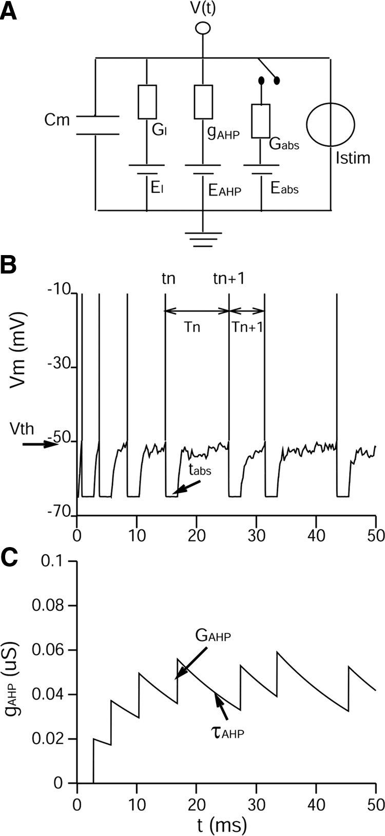
Model structure and model responses to a step current. A: the electric circuit representation of the model. Model parameters are listed in Table 1. B: model membrane potentials in response to a step-current with stochastically fluctuating amplitude (Ī = 1.0 nA; σ_I = 0.2 nA). The model has G_AHP = 0.02 μS and τ_AHP = 20 ms. Vertical bars show the times that the model membrane exceeds the threshold (−50 mV). As indicated, t_n is the spike time of the n_th discharge and T_n is the duration of the following interval. C: accumulated conductance of the adaptation channel g_AHP(t), which increases by G_AHP after the absolute refractory period t_abs and decays toward 0 with a time constant τ_AHP.

We studied effects of the adaptation channel parameters, G_AHP and τ_AHP, on model responses to stochastic currents and to stochastic synaptic inputs. In the synaptic case, the current source in Fig. 1A was replaced by synaptic conductance channels coupled to the inputs. Combinations of the two adaptation channel parameters, in which each parameter took either a high or a low value, led to four distinct cell types. Other membrane parameters were kept fixed across the different model cells. The variable parameter values of the model membrane, specifically G_AHP and τ_AHP, were adjusted to match four example LSO neurons in responses to ipsilateral tonal stimuli (Tsuchitani and Johnson 1985). Model parameters are listed in Table 1. It needs to be emphasized that, for simple spiking models like the one used in this study, model parameters were evaluated based on the model discharge statistics. Because the spiking activity of a model cell is determined by the relationship between the spike threshold and the effective input strength, all model parameter values were chosen relative to an arbitrarily assumed spike threshold.

Table 1.

Membrane properties and synaptic input parameters

Membrane properties
	Cell 1 (Glo: τhi)	Cell 2 (Ghi: τhi)	Cell 3 (Glo: τlo)	Cell 4 (Ghi: τlo)
GAHP(μS)	0.02	0.05	0.02	0.08
τAHP(ms)	20	20	5	5
Cm = 31.4 pF; GL = 0.0314 μS: τm = Cm/GL = 1 ms: Gabs = 10 μS; tabs = 2 ms;
El = EAHP = Eabs = Vrest = −65 mV; Vth = −50 mV;
Synapses
τE = τI = 1 ms; τrise = 0.1 ms; GE* = 1.2 nS; GI* = 3 nS; EE = 0 mV; EI = −70 mV;
*Unitary E and I synaptic current balanced at Vth: GEτE(Vth − EE) + GIτI(Vth − EI) = 0

Parameters for input rate-level functions
Sound level (dB)	0	10	20	30	40	50	60	70
C(sp/sec)	81	351	532	653	734	789	825	850

Current and synaptic stimuli

Previous studies have shown that LSO cells receive ipsilateral excitation from the anteroventral cochlear nucleus (AVCN) and contralateral inhibition from the medial nucleus of the trapezoid body (MNTB) (Cant and Casseday 1986; Finlayson and Caspary 1989; Glendenning et al. 1985; Sanes 1990; Spangler et al. 1985). In this study, the four LSO cell models were driven either by injected stochastic currents with different strengths or by conductance-activated synaptic currents with different driven rates.

Injected current inputs were used to simulate and study the discharge properties of LSO cells to ipsilateral excitatory stimuli. A model cell received a random discrete current at a sampling rate of 4,000 Hz. The amplitude of the current within each sample period (0.25 ms) was a Gaussian random variable with a mean of Ī and an SD of σ_I; and both Ī and σ_I were time-invariant (i.e., the input is stationary). Simulations tested model responses to currents with different combinations of values of Ī and σ_I, which greatly simplified the characteristics of afferent activity in the LSO and allowed analytical evaluations of the effects of model parameters.

Synaptic currents were used to simulate responses of LSO cells to bilateral acoustic stimuli with various ILDs. In these binaural simulation cases, discrete input events were generated according to input rate functions of nonstationary Poisson processes, which described the rates of arrivals of excitatory and inhibitory synaptic events. The acoustic stimulus simulated is a narrow-band, frozen noise with a bandwidth of 500 Hz and a center frequency of 10 kHz. With the assumption that the responses of LSO neurons are temporally locked to the envelope, not the fine structure of sound inputs (Joris and Yin 1998), the synaptic events were derived directly from the envelopes of the input stimulus in three steps. First, the envelope of the narrow-band noise was extracted using Hilbert transform methods in Matlab software. Second, the envelope waveform was normalized to have a maximum of unity, scaled by a sound-level dependent parameter C for excitatory and inhibitory sound levels, and used as the time-varying input-rate functions for excitatory and inhibitory inputs. Third, event times of all input fibers were independently generated from the input-rate functions with no dead-time assumed for the input. The parameter C, corresponding to the peak value of the input-rate function, monotonically increased with the sound level L from 0 to 70 dB SPL as specified in Table 1.

For these synaptic inputs, each input event triggered a conductance change of a synapse in the cell model. For both excitation and inhibition, the synaptic conductance g(t) was simulated as a linear combination of two exponentials with specified peak conductance G_E (and G_I) at time t_p. For example, for excitatory synapses, $g\left(t\right)=\frac{G_{\text{E}}}{\text{gnorm}}\left[\exp \left(-t/{\tau }_{\text{E}}\right)-\exp \left(-t/{\tau }_{\text{rise}}\right)\right]$, where the normalization factor gnorm was chosen to be gnorm = exp(−t_p/τ_E)−exp(−t_p/τ_rise) so that the peak conductance was G_E and the time of the peak was $t_p=\frac{{\tau }_{\text{rise}}{\tau }_{\text{E}}}{{\tau }_{\text{E}}-{\tau }_{\text{rise}}}\ln \frac{{\tau }_{\text{E}}}{{\tau }_{\text{rise}}}\text{with}\hspace{0.17em}{\tau }_{\text{E}}>{\tau }_{\text{rise}}$. The model had 50 excitatory and 50 inhibitory synapses, using the same time constants (τ_rise = 0.1 ms and τ_E = τ_I = 1 ms), but different peak conductance G_E and G_I as specified in Table 1. The synaptic inputs with arbitrarily chosen afferent numbers produced a smooth depolarization in the model membrane potential.

Measurements and data analysis

Model responses to repetitive presentations of the stimuli described above were used to analyze discharge properties. The duration of the stimulus (200 ms for current stimuli and 500 ms for synaptic stimuli) and the number of repetitions (200 for current stimuli and 50 for synaptic stimuli) were chosen to yield sufficient statistical information to compare model responses to results from electrophysiological experiments. The model was simulated in the NEURON environment (Hines and Carnevale 1997, 2000) using the backward Euler integration method with a fixed numerical time step of 25 μs.

Measurements of model discharge patterns to current inputs

The discharge rate, the mean μ_T, and the SD σ_T of ISIs, as well as the associated CV (CV = σ_T/μ_T), were calculated based on discharge times {t_n} and time intervals {T_n} between consecutive discharges, as extracted from the simulations (cf., Fig. 1B). Furthermore, to compare with empirical measurements (Tsuchitani and Johnson 1985), we analyzed model responses in different time segments. Responses during the initial 40 ms of a stimulus were used to measure the poststimulus time histograms (PSTHs) with a binwidth 0.25 ms, as well as the mean intervals (μ_T) as a function of time with a binwidth of 2 ms, using the method described by Young et al. (1988). Responses during the sustained portion of responses (responses occurring after the 1st 40 ms of a stimulus) were assumed to be stationary and were used to compute the ISIH and the associated recovery function H(t) (i.e., the Hazard function). More specifically, the ISIH was generated by binning ISIs relative to a maximum interval T with a binwidth Δt (Δt = 0.2 ms) such that $\text{ISIH}\left(\text{i}\right)=\frac{N_{\text{i}}}{\text{N}\Delta \text{t}}$, where i is the a time index in units of Δt, N is the total number of intervals, and N_i is the number of intervals whose values are within the range [iΔt, (i + 1)Δt] for i = 0, 1, … , K, and $K=\frac{T}{\Delta t}-1$. The recovery function H(t) was generated by normalizing ISIH(i) by the probability that no events occur before i time units: $H\left(\text{i}\right)=\frac{N_{\text{i}}/\text{N}}{\left[\left(\text{N}-{\displaystyle {\sum }_{\text{j}=\text{i}}^{\text{i}-1}{N}_{\text{j}}}\right)/\text{N}\right]\Delta \text{t}}=\frac{{\text{N}}_{\text{i}}/\text{N}}{\left[\left({\displaystyle {\sum }_{\text{j}=\text{i}}^{\text{K}}{N}_{\text{j}}}\right)/\text{N}\right]\Delta \text{t}}$. The estimations of H(i) stopped when $\frac{{\displaystyle {\sum }_{\text{j}=\text{i}}^{\text{K}}{N}_{\text{j}}}}{\text{N}}<0.05$ to avoid a small-denominator effect. Note that both functions ISIH and H were normalized by dividing by Δt, resulting in the usual units of inverse seconds.

Because the adaptation-channel activity persisted across spike boundaries, the membrane integration time depended on previous spike activity (i.e., the discharge process was nonrenewal). A large residual conductance of the adaptation channel after t_abs, which may have resulted from a previous short interval (T_n), delayed the next event time causing a larger T_{n + 1}. A preponderance of short-long or long-short pairs of intervals produced a negative serial correlation between all neighboring intervals, as observed in the empirical measurements (Tsuchitani and Johnson 1985). Because they are based on the first-order properties of intervals, the ISIH and H do not capture the cross-interval dependence in a nonrenewal process. To study the dependence between neighboring intervals [(T₁, T₂), (T₂, T₃), … , (T_N-1, T_N)], we estimated the conditional mean of ISIs given the value of the previous interval in model responses (Rodieck et al. 1962). When plotted as a function of the size of the previous interval, this conditional mean plot provides graphical displays of the serial dependence between intervals. Furthermore, the first-order serial correlation coefficient (ρ₁) was calculated to quantify the degree of the correlation in spike intervals (Cox and Lewis 1966; Perkel et al. 1967) given that the process is stationary; specifically, ρ₁ is given by ${\rho }_1=\frac{COV\left(T_{\text{i}},T_{\text{i}-\text{1}}\right)}{VAR\left(T\right)}=\left(\frac{1}{N-1}{\displaystyle \sum _{i=2}^N{T}_i{T}_{i-\text{1}}-}{\mu }_T^2\right)/{\sigma }_T^2$. The intervals were considered correlated if the ρ₁ value was significantly different (level of confidence 99%) than that measured for the randomly shuffled interval sequence, in which any sequential dependence in the original sequence was destroyed. Interval correlation measurements were only applied to simulations with more than four intervals per trial during the sustained portion of responses.

Measurements of model responses to synaptic inputs

Excitatory and inhibitory synapses were driven by simulated AVCN activity at multiple stimulus sound-pressure levels (0∼70 dB SPLs). The rate-level functions (i.e., parameter C in Table 1) for synaptic inputs were the same for excitation and inhibition; no time-delay difference was imposed between excitatory and inhibitory inputs. To generate an ILD, the ipsilateral excitation level was held constant at 50 dB, whereas the contralateral inhibition level was varied from 0 to 50 dB, corresponding to ILDs from −50 to 0 dB. Negative ILD values indicate more intense acoustic signal at the ipsilateral (excitatory) ear.

The discharge rate was measured at multiple ipsilateral and ILD levels. The PSTH responses of the four model cells were generated by counting spikes in 0.2-ms time windows as a function of time and smoothing these time series using one of two alternative Gaussian filters. Each filter had a mean of zero and a SD of either 0.2 or 5ms, depending on the analysis, and was truncated at ±3 SD with unit energy. Two sets of correlation coefficients (r) were measured to compare the temporal response properties among model cells: the sample correlation coefficients 1) between the input function and smoothed PSTH of a model cell and 2) between the smoothed PSTHs of two model cells to identical inputs. All correlation coefficients were collected at multiple ipsilateral sound levels and ILDs.

In all simulations with synaptic inputs, the synaptic parameters were chosen so that mean currents through single excitatory and inhibitory synapses cancelled each other at the threshold membrane potential V_th, i.e., I_E + I_I ≈ G_Eτ_E(V_th − E_E) + G_Iτ_I(V_th − E_I) = 0, as used in balanced inhibition models for cortical neurons (Shadlen and Newsome 1994; Troyer and Miller 1997). Here, the synaptic conductance was approximated by its mean (G_Eτ_E or G_Iτ_I). As a result of this constraint, the model response reached a minimum at zero ILD because of balanced synaptic currents at equal acoustic levels between the ipsilateral and contralateral ears. Models yielded no response at positive ILDs (i.e., more inhibition), and thus simulations are not presented for positive ILD values.

Analysis of model outputs with respect to model parameters

Because the statistics of model discharges link directly to underlying membrane integration dynamics, we used simplifying assumptions to derive expressions for the subthreshold membrane potential as a function of model parameters. These simplified expressions allow more intuitive understanding and comparison with simulation results. The model membrane potential following the absolute refractory period in response to a fixed current I_stim was first described by the complete equation

$$C_{\text{m}}\frac{\text{d}V\left(t\right)}{\text{d}t}+G_{\text{L}}\left[\text{V}\left(\text{t}\right)-{\text{E}}_{\text{1}}\right]+\left({\tilde{g}}_{\text{AHP}}+\Delta g_{\text{AHP}}\right)\left[\text{V}\left(\text{t}\right)-{\text{E}}_{\text{AHP}}\right]={\text{I}}_{\text{stim}}$$ (1)

where the time origin was reset to zero for analysis purposes and ḡ_AHP denoted the average accumulation of g_AHP(t) caused by previous spikes. Because it was assumed that E_l = E_AHP = V_rest in this model, Eq. 1 was rewritten as

$$C_{\text{m}}\frac{dv\left(t\right)}{dt}+G_{\text{L}}^{\prime }\text{v}\left(\text{t}\right)+\Delta g_{\text{AHP}}\text{v}\left(\text{t}\right)={\text{I}}_{\text{stim}}$$ (2)

with v(t) = V(t) − V_rest and G′_L = G_L + g̃_AHP. Furthermore, because the membrane time constant τ′_m associated with G′_L was so small [τ′_m equaled C_m/G_L and was <1 ms, much smaller than τ_AHP (5 or 20 ms)], the capacitance current was quickly dispersed; thus it was assumed that $C_{\text{m}}\frac{dv\left(t\right)}{dt}\approx 0$. With these considerations, the membrane potential v(t) in Eq. 2 can be approximated, following Smith and Goldberg (1986); as $v\left(t\right)=\frac{I_{\text{stim}}}{{\text{G}}_{\text{L}}^{\prime }+\Delta g_{\text{AHP}}}=\frac{{\text{I}}_{\text{stim}}}{{\text{G}}_{\text{L}}^{\prime }+{\text{G}}_{\text{AHP}}\exp \left(-t/{\tau }_{\text{AHP}}\right)}$. Finally, we linearly expanded v(t) around t = 0 using Taylor series expansions of exp(−t)and of $\frac{1}{1-t}$. Then, it can be shown that for 0 ≤ t < τ_AHP

$$v\left(t\right)=\frac{I_{\text{stim}}}{{\text{G}}_{\text{L}}^{\prime }+{\text{G}}_{\text{AHP}}\exp \left(-t/{\tau }_{\text{AHP}}\right)}\approx \frac{{\text{I}}_{\text{stim}}}{{\text{G}}_{\text{L}}^{\prime }+{\text{G}}_{\text{AHP}}\exp \left(1-t/{\tau }_{\text{AHP}}\right)}\approx \frac{{\text{I}}_{\text{stim}}}{\left({\text{G}}_{\text{L}}^{\prime }+{\text{G}}_{\text{AHP}}\right)}\left[1+\frac{G_{\text{AHP}}}{{\tau }_{\text{AHP}}\left({\text{G}}_{\text{L}}^{\prime }+{\text{G}}_{\text{AHP}}\right)}t\right]=v_0+s_{0}t$$ (3)

With the above simplifying assumptions and analysis as given in Eq. 3, the subthreshold membrane potential v(t) following the absolute refractory period was approximately a linear ramping function with initial value v₀, where $v_0=\frac{I_{\text{stim}}}{{\text{G}}_{\text{L}}^{\prime }+{\text{G}}_{\text{AHP}}}$ and slope s₀, where $s_0=\frac{dv\left(t\right)}{dt}=\frac{I_{\text{stim}}{G}_{\text{AHP}}}{{\tau }_{\text{AHP}}{\left({\text{G}}_{\text{L}}^{\prime }+{\text{G}}_{\text{AHP}}\right)}^2}$. The parameters v₀ and s₀, associated as shown with the input and model parameters, were used to explain model outputs in the results sections of this paper.

RESULTS

Responses of model cells to ipsilateral excitatory inputs

EFFECTS OF AHP PARAMETERS ON THE SUBTHRESHOLD VOLTAGE TRAJECTORY.

In an integrate-and-fire model, properties of the spike interval (i.e., the 1st passage time to a voltage threshold) depend on the subthreshold voltage trajectory V(t), predominantly its initial value and slope (Geisler and Goldberg 1966; Troyer and Miller 1997). The change of the membrane conductance, which is introduced by the adaptation channel for AHP in our model, alters the voltage trajectory and thereby affects the spike interval. Figure 2 shows subthreshold voltage traces of model cells for different values of G_AHP and τ_AHP in response to a constant depolarizing step-current I_stim applied at time 0. The voltage resets to the resting potential after reaching the threshold (V_th = −50 mV) and the adaptation channel opens after the absolute refractory period (2 ms). In comparison to the first discharge event, which is not influenced by the adaptation conductance, the voltage trajectory during the second discharge event undergoes much longer integration time and is composed of a fast and then slow rising phase. The fast rising phase results from the quick charging of the capacitor (the effective membrane time constant is less than 1 ms) and the slow rising phase results from the slow decrease of conductance in the adaptation channel g_AHP(t) (τ_AHP ranges between 5 and 20 ms). Here we focus on two properties of the V(t) trajectory that are associated with adaptation channel activity, the value of V(t) at the end of the fast phase and the slope of V(t) during the slow phase, which are denoted as v₀ and s₀, respectively, at the end of methods. As shown in Fig. 2A, a longer τ_AHP leads to a shallower slope, whereas v₀ is not affected by τ_AHP. In contrast, as shown in Fig. 2B, a larger G_AHP reduces the size of v₀ and slightly lowers s₀. Figure 2C shows that the strength of the current I_stim influences both the v₀ and s₀ of the V(t) trajectory—a stronger current leads to a steeper slope and a larger v₀. Finally, note that different parameter combinations of G_AHP and τ_AHP yield V(t) with different trajectories during the ongoing responses for the same current input (Fig. 2D), even when the average spike intervals are similar in the two conditions as shown.

Fig. 2.

Subthreshold voltage trajectories to a step-current for several values of the model parameters G_AHP and τ_AHP. A: the value of τ_AHP affects the slope of the voltage trajectory (G_AHP = 0.08 μS and I_stim = 1 nA). B: the value of G_AHP affects membrane potential v₀ at the end of the fast-rising phase (τ_AHP = 5 ms and I_stim = 1 nA). C: the current strength I_stim affects both the initial value v₀ and slope s₀ of the voltage trajectory (G_AHP = 0.08 μS and τ_AHP = 5 ms). D: different combinations of parameter values (G_AHP and τ_AHP) that lead to voltage trajectories with different v₀ and s₀ but to similar interval between firings (I_stim = 1 nA).

This model behavior can be understood by the linear expansion of V(t) relative to V_rest [v(t) = V(t) − V_rest] when the membrane time constant τ′_m is much smaller than τ_AHP. In this case, it is shown above (Eq. 3) that $v_0=\frac{I_{\text{stim}}}{{\text{G}}_{\text{L}}^{\prime }+{\text{G}}_{\text{AHP}}}$ and $s_0=\frac{I_{\text{stim}}{G}_{\text{AHP}}}{{\tau }_{\text{AHP}}{\left({\text{G}}_{\text{L}}^{\prime }+{\text{G}}_{\text{AHP}}\right)}^2}$, consistent with simulation results. Because both the adaptation channel activity and the input strength influence the membrane potential integration, but in different ways, we predict that models with different combinations of G_AHP and τ_AHP values would exhibit different temporal discharge patterns and that AHP effects and input effects are distinguishable. In the following simulations, we measured spike interval statistics of the four model cells during onset and sustained phases of responses. These results were compared with those of exemplar and population neurons in the LSO (Tsuchitani 1982; Tsuchitani and Johnson 1985).

Effects of AHP parameters on PSTHs

Physiological studies classified LSO cells into fast and slow chopper units (Tsuchitani 1982) based on their response to ipsilateral pure-tone stimuli. During the onset phase of responses, fast choppers exhibit narrower peaks separated by shorter interpeak intervals, and therefore faster chopping frequencies, relative to slow choppers. Based on the results in Fig. 2, we expected that shorter spike intervals of fast choppers are caused by a near-threshold (large) v₀ associated with a smaller G_AHP and, furthermore, that different slopes of V(t) associated with τ_AHP may lead to different adaptation rates in the onset PSTHs. To test this hypothesis, we simulated four model cells with large/small G_AHP and long/short τ_AHP (model parameters in Table 1 were chosen to match model interval distributions with the neural data shown in later results).

Figure 3 shows the PSTHs (<40 ms) of four model cells (columns) to stochastic current inputs at three different strength levels (different values of Ī are shown in the top 3 rows). The evolutions of the mean ISI μ_T in time (<20 ms) are shown at the bottom row; smaller μ_T values indicate faster chopping frequencies in PSTHs. Consistent with our hypothesis, for the same Ī values, cells 1 and 3 (with smaller G_AHP) exhibit fast chopping patterns, whereas cells 2 and 4 (with larger G_AHP) exhibit slow chopping patterns. (Note that the vertical scale in the second panel of the bottom row is different.) Because the size of v₀ also increases with Ī (cf., Eq. 3), a faster chopping frequency is seen at higher current strength as well. Furthermore, the values of μ_T increase more rapidly over time for cells 1 and 2 (with larger τ_AHP) than cells 3 and 4 (with smaller τ_AHP), indicating faster firing-rate adaptation. The adaptation occurs because the average membrane conductance G^′_L increases over time because of accumulation in g_AHP(t), so that the v₀ value after each spike gradually decreases from the threshold, causing a longer interval to the next event. With larger τ_AHP values, model g_AHP(t) builds up more rapidly (Liu and Wang 2001). This explains faster adaptation in responses of model cells 1 and 2 than those of cells 3 and 4.

Fig. 3.

Chopper responses in model cells. In the first three rows, onset poststimulus time histograms (PSTHs) of the 4 model cells (columns) are shown for stochastic current stimuli at different strengths (rows). Model cells 1 and 3 show fast-chopper response patterns, and model cells 2 and 4 show slow-chopper response patterns. The chopping frequency increases with the mean current strength Ī (σ_I is fixed at 0.4 nA). In the bottom row, the short-time-averaged interval between firings μ_T is plotted as a function of time since the onset of the stimulus burst. The magnitude of μ_T reflects the chopping interval with the stimulus current level as a parameter.

Effects of AHP parameters on interval distributions in steady state

Responses of fast and slow LSO chopper units differ not only in their initial chopping response patterns (<40 ms) but also in spike interval distributions in the steady state (>40 ms). Observed interval distributions are skewed toward short intervals for fast choppers and nearly symmetrical in shape for slow choppers (Tsuchitani and Johnson 1985). For a renewal process, the recovery or hazard function (which is determined by the interval distribution) completely describes the behavior of the event generation by depicting the conditional response probability (Johnson 1996). Figure 4 shows (left 2 columns) the ISIHs and corresponding recovery functions for the four model cells during the stationary sustained-response phase in response to stochastic current inputs with increasing strength (current levels increase from curves A to curves D). Figure 4 also shows (right column) recovery functions for two fast-chopper units (86-1F and 51-1E) and two slow-chopper units (128-1A and 42-1A) as measured from LSO data (Tsuchitani and Johnson 1985) in response to ipsilateral tone-burst stimuli with increasing intensity (levels increase from A to E). For both model cells and LSO chopper units, the predominance of short spike intervals increases with input current/sound level as shown in the recovery functions (and also manifested by the shifts of the centers of the ISIH distributions to shorter intervals for model cells). Consistent with the neural responses, fast choppers (model cells 1 and 3) exhibit sharp rises in recovery functions at short intervals (concave downward shapes) and skewed ISIHs, while slow choppers (model cells 2 and 4) exhibit slow rises in recovery functions at short intervals (concave upward shapes) and nearly symmetrical ISIHs, even at high-input levels. Within either the fast or slow chopper type, the ISIHs are broader for model cells with a long τ_AHP (i.e., for model cells 1 and 2). An intuitive interpretation can be obtained based on the subthreshold membrane trajectory V(t) as explored in Fig. 2. A higher v₀ value of V(t) leads to a higher probability of short intervals in ISIHs, and a shallower slope of V(t) enables threshold crossing in a greater range of time and thus a broader spike interval distribution.

Fig. 4.

Spike interval statistics for the 4 model cells and 4 representative lateral superior olive (LSO) chopper units. Left and middle columns: the interspike interval histograms (ISIHs) and recovery functions, respectively, of model cells to current stimuli. For curves A–D, mean currents Ī were 0.6, 1.0, 1.4, and 1.6 nA for model cells 1, 3, and 4 and 1.2, 1.6, 2.0, and 3.0 nA for model cell 2 (σ_I is fixed at 0.4 nA in all simulations in this figure). Right panels: the empirical recovery functions of 2 fast and 2 slow chopper units to ipsilateral tone-burst stimuli (Tsuchitani and Johnson 1985). Sound pressure level increases from A to E covering a range of 50 dB SPL above the unit threshold.

In the preceding results, fitting a variety of neural responses by varying only two parameters G_AHP and τ_AHP suggests diversity in the amplitude and dynamics of membrane AHP among LSO neurons. However, an alternative explanation of the neural data may be that LSO cells may have similar membrane properties (i.e., with the same AHP characteristics), but simply receive different amounts of afferent inputs. Hypothetically, cells with weak inputs could be slow choppers and cells with strong inputs could be fast choppers. This alternative reasoning is supported by the observation that changing the current strength alone varies the chopping frequencies (Fig. 3) and shape of ISIHs (Fig. 4) and alters the voltage trajectory in ways similar to those achieved by varying G_AHP and τ_AHP independently (Fig. 2C). The input-strength hypothesis is rejected by the dependence of serial correlation in adjacent intervals described in the next paragraphs. Specifically, it is shown below that membrane factors, not input strength, determine the response dynamics when the nonrenewal discharge patterns in the LSO are taken into account.

Effects of AHP parameters on serial dependence of intervals in steady state

The nonrenewal nature of spike generation in the LSO was studied with a focus on the serial dependence between intervals from responses of chopper units. Figure 5 shows the conditional mean measurements for spike intervals of the four model cells and of the four LSO chopper units (same units and stimuli as in Fig. 4) at various input levels. A negative correlation between adjacent intervals (e.g., T_n and T_n+1) is manifested by the negative slope in the relationship between the length of the current interval (abscissa) and the mean length of the next interval (ordinate). In the neural data, fast-chopper unit 86-1F and slow-chopper unit 128-1A show similar, strong negative serial correlations over a range of intervals at all sound levels. In contrast, only long intervals of fast-chopper unit 51-1E (upper sets of points corresponding to low sound levels) and short intervals of slow-chopper unit 42-1A (lower sets of points corresponding to high sound levels) show modest correlation. The four model cells show the same trends, matching the neural data.

Fig. 5.

Comparisons between conditional mean measurements E[T_{n + I}|T_n] for the 4 model cells (left) and the 4 LSO chopper units shown in Fig. 4 (right). Model cells 1 and 2 exhibit stronger serial correlation between intervals. The degree and range of interval correlations are similar between model cells and LSO chopper units. The stimulus conditions for model cells and LSO chopper units are the same as those in Fig. 4.

Notably, the hypothesis that the LSO response patterns are determined by input strength would predict a similar degree of interval correlation at a given T_n between the same-type chopper units. This is observed in neither neural nor model responses. We found that serial correlations between adjacent intervals in model cells are caused by the residual adaptation conductance ḡ_AHP, which corresponds to the average accumulation of g_AHP(t) caused by previous spikes. A large ḡ_AHP value arising from a short previous interval T_n tends to extend the next interval T_n+1 by decreasing v₀ values, and longer previous intervals tend to decrease the ḡ_AHP values and shorten the next interval. Moreover, residual ḡ_AHP would vary with T_n and affect T_n+1 only when the decay of the adaptation channel (related to τ_AHP) outlasts the time to the next firing (T_n). This explains strong interval correlations at all levels in model cells 1 and 2 (when τ_AHP is longer than T_n) and weak interval correlations at long intervals in model cell 4 (when τ_AHP is shorter than T_n). Thus various discharge properties for slow and fast choppers are predominantly caused by differences in membrane-recovery dynamics in the LSO. Along with results of the role of G_AHP in determining the initial chopping frequencies (Fig. 3), we conclude that LSO cells are heterogeneous in their membrane properties with the parameter G_AHP showing different strength and the parameter τ_AHP showing different duration of membrane adaptation.

Comparisons between model responses and a population of LSO neurons

Although models with different G_AHP and τ_AHP produced good matches with in vivo responses of four chopper units in the LSO, one may ask how these parameter values capture the full diversity in discharge properties in the LSO. To answer this question, we compared qualitatively the model results to those of a population of LSO chopper cells (6 fast and 14 slow choppers; Tsuchitani and Johnson 1985) at different input levels. For comparison, the results of modeling simulation without the AHP channel activity (which is a LIF model) are included as well. Figure 6 shows the level dependence of discharge rate, response regularity (measured by the CV), and the serial correlation coefficient (ρ_I) of intervals for the four model cells (left column) and LSO population responses (right column); units were roughly categorized into fast or slow choppers by Tsuchitani and Johnson (1985). Clear segregations between responses of fast and slow choppers are seen in all three metrics. Grouping these metrics measured from model fast/slow choppers yields trends comparable to those in the neural data.

Fig. 6.

Comparisons between the discharge rates, CVs, and serial correlation coefficients (ρ₁) of model responses to stochastic current stimuli (left) and of a population of LSO chopper units to ipsilateral tone bursts (right). The responses of model cells with afterhyperpolarization (AHP) show similar trends with the neural data from Tsuchitani and Johnson (1985). The responses of the model cell without AHP are depicted in dash lines. Ī ranges from 0.4 to 3.0 nA in steps of 0.2 nA (σ_I is fixed at 0.4 nA). The significance of nonzero ρ_I was accepted at a level of confidence 99%; insignificant values are marked with asterisks for the model results.

Considering discharge rates, the rate-level functions for fast choppers are steeper (high gain) than those for slow choppers (low gain) for both model cells (Fig. 6A) and LSO chopper units (Fig. 6D). Firing rates in model cells are affected directly by the shunting effect of the accumulated adaptation conductance ḡ_AHP (for an exponential function g_AHP(t), ḡ_AHP ∝ G_AHP × τ_AHP): the larger the accumulation, the lower the discharge rate (Liu and Wang 2001). Therefore model cell 2 (long τ_AHP and large G_AHP) has the lowest discharge rates, model cell 3 (short τ_AHP and small G_AHP) has the highest discharge rate, and model cell 1 and model cell 4 (the same product of G_AHP and τ_AHP, but very different interval distributions) exhibit almost identical rate-level functions. All four model cells discharge less than the LIF model without AHP (Fig. 6A, dashed line).

Considering the CV, the discharge regularity increases with sound level (i.e., CV decreases) for fast choppers and remains relatively insensitive to sound level for slow choppers (Fig. 6, B and E). The trend in the model fast choppers is typical for LIF models (Fig. 6B, dashed line), in which the threshold-crossing is random in response to a weak input and deterministic in time (equal to the absolute refractory period) in response to a strong input. For model slow choppers, because the width (σ_T) and mean (μ_T) of their ISIHs decrease with increases in the current strength at the level applied (Fig. 4), the model CV values (CV = σ_T/μ_T) remain relatively insensitive to input level. In addition, for the same chopper type (similar G_AHP), models with a shorter τ_AHP (cells 3 and 4) respond more regularly (smaller CV) than those with a longer τ_AHP (cells 1 and 2), because the former have narrower ISIHs (σ_T) (Fig. 4, C and D).

Considering the serial correlation of intervals, results show that spike interval correlation is absent in the LIF model responses (Fig. 6C, dashed line) and that the negative correlation between intervals initially becomes stronger as the stimulus level increases (negative initial slopes) for both fast and slow choppers and becomes weaker as the stimulus level further increases (positive slopes at high levels) for fast choppers (Fig. 6, C and F). Neighboring discharges in model responses show weak negative correlations at two extremes: 1) at very low input levels, because the τ_AHP value is shorter than the average spike interval (μ_T) and thus AHP does not carry memory between successive spike intervals; 2) at high-input levels for fast choppers, because the τ_AHP value is much longer than μ_T and the amount of the decay in g_AHP(t) is too small to affect the next interval. In models, negative correlations between neighboring intervals are strongest when the effective duration of the AHP effect (i.e., τ_AHP) is comparable to μ_T. Because model cells have different values of τ_AHP and μ_T, the maximal correlation occurs at different input levels.

Overall, the progressions of these three response metrics with level are consistent with those of the neural data and the data fitting was achieved solely by using different G_AHP and τ_AHP values in model cells. The range of these parameter values may largely reflect the diversity of membrane properties in the LSO. Both data and model responses strongly suggest that, besides the average rate, temporal patterns of responses (the spike interval variations and correlations between adjacent intervals) also vary with sound level in ways that are different between fast and slow choppers. However, the functional significance of the metrics CV and serial correlation for the neural code is not clear. In later sections, we directly evaluated the rate and temporal coding of ipsilateral and bilateral sound level in the LSO in terms of the effects of the AHP parameters.

Effects of variability in stimulus amplitude on interval statistics

The previous results simulated LSO responses to tonal stimuli at different sound levels by varying the strength of current amplitude (Ī), while the SD of current amplitude (σ_I) was held constant in all experiments to fix the stimulus noise. However, fluctuations in afferent inputs to the LSO in response to acoustic stimuli are likely proportional to the stimulus level and affected by the afferent properties, such as numbers of synapses or the size of synaptic conductance. Here, the effects of the current fluctuation σ_I were studied separately for a fixed Ī.

Figure 7 shows the effects of σ₁ on the discharge rate, regularity (CV), and serial correlation coefficient (ρ₁) of spike intervals for the four model cells to current inputs with different σ_I. In A and B, results show that both the discharge rates and the CV values increase with σ_I (i.e., noisy inputs cause more irregular firings), with the exception of the model cell 3 whose discharge rate is insensitive to σ_I. Furthermore, input noise is necessary for inducing the correlated neural discharges. In C, constant step current (σ_I = 0) elicits no correlation between successive spike intervals. The amplitude of input noise also affects interval correlation, which decreases with the increase of σ_I. Recall that the negative interval correlation results from the residual adaptation conductance ḡ_AHP from previous spikes; changes in ḡ_AHP lead to different initial potential values of v₀ over time (Eq. 3). As σ_I increases, the uncertainty in v₀ depends less on ḡ_AHP and more on the noisy I_stim, whose fluctuation is independent of discharge history. Hence, the reduced influence of ḡ_AHP leads to reduced serial correlations between successive intervals. The reduction in spike interval correlation is most evident in the responses of model cell 1, because a small G_AHP amplifies the impact of σ_I on v₀. Hence, the AHP channel characteristics may also affect the neural responses to noise factors in input amplitude. Similar firing-rate regulation by AHP has been observed in responses of neocortical neurons to noisy current inputs (Higgs et al. 2006).

Fig. 7.

The response properties of 4 model cells to stochastic current inputs with different σ_I. Ī = 1.4 nA. Model cells are marked by symbols as follows: cell 1(○), cell 2 (◽), cell 3(), and cell 4 (♢). A: discharge rates of model cells slightly increase with σ_I. B: models respond more irregularly as σ_I increases. C: the serial correlation between spike intervals (ρ₁) decreases with increase of nonzero σ₁, which is more evident in model cell 1 because of a small G_AHP. All nonzero ρ₁ values are significant (with the level of confidence 99%).

Responses of model cells to bilateral synaptic inputs

The interaction between input strengths of excitation and inhibition has been proposed as the neuronal mechanism for the ILD sensitivity at a single-neuron level (see Irvine 1992 and Tollin 2003 for reviews). To address the question of how membrane heterogeneity contributes to neural coding of sound levels, especially ILDs, we compared responses of the four model cells to the envelope of a frozen band-pass noise for both ipsilateral alone (excitation) and bilateral (excitation and inhibition) stimulation conditions. The band-pass noise was generated digitally by band-pass filtering a white noise around 10 kHz with a bandwidth of 500 Hz (as shown in Fig. 8, A and B). The envelope waveform of the filtered noise was extracted using the Hilbert Transform (as shown by the gray line in Fig. 8B) and used to describe the input-rate function (see methods for details). Figure 8C shows the power spectrum of the envelope waveform (512-point FFT). Because the modulation depth of the envelope of narrow-band noise is affected by the instantaneous phase interaction between fine-structure frequencies, the envelope waveform is not simply related to the bandwidth of the original waveform. The envelope extraction approximates the half-wave rectification and low-pass filtering of sound during the peripheral auditory processing.

Fig. 8.

The PSTHs of model cells in response to a frozen, narrowband–noise waveform. A and B: the original and filtered noise around 10 kHz with a bandwidth of 500 Hz. The gray line shows the envelope waveform exacted using Hilbert transform. C: the power spectrum of the envelope waveform (512-point FFT). D and E: responses to the ipsilateral stimulus alone at 50 dB and to the bilateral stimuli (corresponding to ipsilateral stimulus at 50 dB and a contralateral stimulus at 10 dB). The thick black lines depict the smoothed PSTHs with a bin size 0.2 ms using a truncated, Gaussian-shaped window (±3 SD wide, and SD = 0.2 ms). The input rate function, with a shape common to all stimuli, is shown in both bottom panels as thin black lines. This function is also plotted with a bin size of 0.2 ms.

To get an intuitive understanding of the differences over cells and stimulation conditions, we first examined the temporal profiles of responses. Figure 8, D and E, shows corresponding segments of PSTHs of four model cells to ipsilateral inputs at 50 dB (left column) and bilateral inputs with ipsilateral level of 50 dB and contralateral level of 10 dB (right column); the common ipsilateral input function is shown by the thin line in each of the two bottom panels. Model responses show chopping patterns and synchronization to the input function. For the four model cells, the overall tracking of the input differs in terms of the similarity between input and response profiles. Contralateral inhibition does not change the general trend of model responses, but does smear the temporal details and reduce the rate of the responses (resulting in less chopping) for all model cells.¹

Detailed examinations show that the membrane AHP influences the rate modulation of a response profile. In particular, model cells 1 and 4, although they have similar firing rates (seen in Fig. 9A), show different depths of modulation between adjacent peaks of PSTHs in response to identical stimuli. As shown in the previous section, the time-varying response rate (which equals the inverse of spike interval) is affected by the immediate history of spiking activities in a nonrenewal process. Because smaller intervals are followed by longer intervals in model cells with greater AHP, a greater rate modulation is observed for model cells 1 and 2 with larger τ_AHP. In Fig. 8, the arrows mark two instances showing similar inputs strength and yet rather different magnitudes and history of responses among model cells. These results indicate that the average rate and temporal patterns of responses may have different level dependence among model cells for both ipsilateral-only and bilateral stimulation conditions.

Fig. 9.

The discharge rate and temporal response measures of model cells in response to ipsilateral synaptic inputs. The ipsilateral level ranges from 0 to 70 dB SPL. Model cells are marked by symbols as follows: cell 1(○), cell 2 (◽), cell 3(), and cell 4 (♢). A: the discharge rate at each level. B: the correlation coefficient between the smoothed PSTHs of model responses and the input rate function at each level. (For the values plotted at 50 dB, these values are correlations between a thick line from the left column of Fig. 8 and the thin lines in the bottom panel of that figure.) C: the correlation coefficient between the smoothed PSTHs of different pairs of model cells at each level (P < 10⁻⁴). In C, the model pair being compared is marked on each curve. (For the values plotted at 50 dB, these are the correlations between pairs of thick lines in the left column of Fig. 8.) The bin size of the input function is 0.2 ms and the SD of the Gaussian smoothing window is 0.2 ms in B1 and C1 and 5 ms in B2 and C2.

Quantitative measures of the simulation results are shown in Figs. 9 (ipsilateral) and 10 (bilateral). We calculated the changes in the firing rate and correlation coefficient r with ipsilateral sound level or ILDs. Two sets of correlations were made, between responses of a model cell and its input function (Figs. 9B and 10B) and between responses of a pair of model cells (Figs. 9C and 10C). The between-cell correlation measures the coincident events among LSO afferents for downstream processing. Because downstream neurons may integrate over temporal windows of different lengths, model PSTHs were convolved with a Gaussian filter with the SD of 0.2 (results are shown in Figs. 9 and 10, B1 and C1) or 5 ms (results are shown in Figs. 9 and 10, B2 and C2). Model cells are identified by symbol in A and B, and model cell pairs are indicated for each curve in C.

Fig. 10.

The discharge rate and temporal response properties of model cells to bilateral synaptic inputs. The ipsilateral level is held at 50 dB and the contralateral level ranges from 0 to 50 dB. Model cells are marked by symbols as follows: cell 1(○), cell 2 (◽), cell 3(), and cell 4 (♢). A: the discharge rate decreases with the increase in contralateral levels. (The ipsilateral alone, 50-dB condition is shown on the left of this panel.) B: the correlation coefficients between the smoothed PSTHs of model response and the ipsilateral input rate function at each level (P < 10⁻⁴). C: the correlation coefficients between the smoothed PSTHs of different pairs of model cells at each level. The model pair being compared is again identified for each curve. (For a contra level of 10 dB, the correlation values in B and C are computed by correlating the thick-lined functions in the right column of Fig. 8 with the thin-line function in the bottom panels or with the other thick-line functions, as described for similar cases in Fig. 9.) The bin size of the input function is 0.2 ms, and the SD of the Gaussian smoothing window is 0.2 ms in B1 and C1 and 5 ms in B2 and C2.

For the ipsilateral-alone input condition, as shown in Fig. 9, the discharge rate varies monotonically with ipsilateral sound level, and the AHP causes different sensitivity to level changes among model cells (different slopes in Fig. 9A), similar to the rate-level functions obtained with current stimuli (Fig. 6A). On the other hand, the temporal measures reveal different level dependence than the rate. First, the correlation values between stimuli and response (shown in B1 and B2) vary little when ipsilateral sound level increases, except for model cell 3 in B1. Because input functions are perfectly correlated at all ipsilateral levels (i.e., scaling does not change correlation), the data indicate that the instantaneous rate modulations of model responses vary in accord with that of the input at all ipsilateral sound levels. This level-invariant property is attributed to the accumulation of the AHP conductance in a model cell, which elevates the threshold of firings as sound level increases, avoiding saturation effects. Consequently, a model cell is able to maintain its dynamic range of responses. As an exception, model cell 3, with the least AHP accumulation (which is proportional to the product of G_AHP and τ_AHP), shows a slight decrease in correlation r with level because of its tonic firings and thus dissimilar temporal patterns with input at higher sound levels when the temporal integration window is short. Second, the between-cell correlation measurements show that similar discharge rates do not predict similar PSTH patterns (6 comparison-pairs are indicated on the right margin of C1 and C2). For example, the responses of model cells 1 and 4 have identical rates but rather different temporal correlations at two different integration resolutions across multiple sound levels (with r < 0.8). Based on the ranking of the value r, model cells 2 and 3 (with different τ_AHP) have the lowest correlation value among all pairs; model cells 1 and 2 (with same large τ_AHP) and model cells 3 and 4 (with same small τ_AHP) have the highest correlation value for the short and long temporal integration window, respectively. These results suggest that the time scale of membrane adaptation determines the similarity in temporal response profiles of different neurons. As observed for input-output functions in B1 and B2, the between-cell correlation remains insensitive to the change of ipsilateral sound level, suggesting level-invariant dissimilarity among model responses, except those with model cell 3 (least AHP accumulation) when the Gaussian filter is short (C1), where the r values decrease with the ipsilateral level. Moreover, the between-cell correlation increases in results using a longer temporal filter (cf., C1 and C2), suggesting that model PSTHs differ in their fast dynamics.

Results for the bilateral stimulation conditions are shown in Fig. 10. Model cells receive ipsilateral excitatory inputs at 50 dB and contralateral inhibitory inputs with levels from 0 to 50 dB; accordingly, the ILD varies from −50 to 0 dB. If inhibition merely decreased the response amplitude, one would expect that when contralateral levels increases, rate response properties would progress opposite to those in Fig. 9. This prediction is seen in the rate-level responses (Fig. 10A)—increasing the contralateral sound level decreases the discharge rates with varying slopes as also seen in the LSO (Boudreau and Tsuchitani 1968). Consequently, model cells respond with different slopes to inhibition levels (i.e., ILDs), because of their different AHP properties. Similar to results in Fig. 9, B1 and B2, temporal correlations between responses and the stimulus remain nearly unchanged with increases in the contralateral level (Fig. 10, B1 and B2), suggesting that inhibition scales, but does not alter, the temporal modulation of model responses. In contrast, despite similar rankings as those in Fig. 9, the between-cell correlations are not level-invariant, especially for those related to model cell 3 with less AHP (dashed lines in Fig. 10, C1 and C2), suggesting that the AHP activity is crucial for the between-cell dissimilarity when stimulated binaurally. Together, results in both ipsilateral and bilateral stimulation conditions indicate that the membrane AHP may contribute to the encoding of the slopes of rate-level and rate-ILD responses, increase (or decrease) the between-cell similarity in temporal response patterns to identical stimuli, and maintain such similarity (or dissimilarity) at variable ipsilateral and/or ILD level.

Balanced excitation and inhibition for “characteristic” ILDs

In this model, membrane AHP affects greatly the slope of a rate-ILD function, but not the threshold of the rate-ILD function, because AHP requires spiking activity. This threshold is referred to as the “characteristic” ILD of an LSO cell, at which a contralateral (inhibitory) input just shuts off responses to an ipsilateral (excitatory) input. Park et al. (1997) found that characteristic ILDs are independent of the excitatory stimulus level in the LSO but not the ILDs associated with the 50% response rate. Although responses at the threshold and slope of a tuning curve both provide information about stimuli (Seung and Sompolinsky 1993; Tollin et al. 2008), the level-invariant feature associated with characteristic ILD is more desirable for encoding ILDs when the overall sound level is not static.

As discussed in methods, characteristic ILD is achieved in our models by using the same input-rate level function for ipsilateral excitation (E) and contralateral inhibition (I), i.e., r_E(L) = r_I(L) and by adjusting excitatory and inhibitory synaptic strengths to yield zero net input strength at zero-decibel ILD, which is chosen for convenience to be the characteristic ILD for all model cells. (More general neural conditions are discussed in the following paragraph.) Figure 11 shows the discharge rate as a function of contralateral level (left) and the normalized rate as a function of ILD (right) for model cell 1 when the ipsilateral level is fixed for three different levels. The discharge rates at 0 ILD (which occur at different contralateral I levels when the ipsilateral E level varies) are insensitive to the E level. The discharge rates at negative ILDs decrease with increases in the E level because of the saturation of E inputs, which reduce the difference between E and I input rates. As a result, a given normalized response shifts to more negative ILDs as the E level increases. These model results are in agreement with in vivo observations (Park et al. 1997). It should also be noted that the shape of the rate-ILD curve as shown in Figs. 9A, 10A, and 11 is affected not only by the membrane properties we have focused on but also by the input rate-level function for excitation and inhibition (i.e., the C values in the bottom row of Table 1). These values incorporate choices for threshold, dynamic range, and saturation level, which were arbitrarily chosen in our C values. For example, the sharp increase of the rate in Fig. 11 at an ILD of −10 dB is caused by the abrupt rise of input-rate near the threshold of input.

Fig. 11.

Dependence of the discharge rate of model cell 1 on contralateral (inhibitory) level for 3 different excitation levels. A: discharge rates decrease with the increase of contralateral inhibition levels. B: same data as in A plotted with interaural level difference (ILD) as the abscissa. The characteristic ILD, where the rate 1st reaches 0 as the contralateral level increases, occurs at 0 ILD for all 3 excitation levels.

How does the population activity of LSO neurons encode different ILDs? Reed and Blum (1990) proposed that the position of near-zero responses of an array of LSO cells (with different characteristic ILDs) signals the ILD of a sound source and thereby the sound location. This hypothesis predicts a systematic distribution of characteristic ILDs in the LSO. Mechanistically, we propose that this can be achieved by simply shifting and scaling input-rate functions between excitation and inhibition as used in our model. Three generalizations of the model parameters are discussed here: 1) arbitrary characteristic ILDs, 2) unbalanced excitatory and inhibitory synapses, and 3) nonzero responses at a given characteristic ILD. First, an arbitrary characteristic ILD can be easily generated by shifting the rate-level function of E or I inputs in the model. For instance, if r_E(L) = r_I(L + α) (argument in dB), complete suppression will occur at an ILD of α dB, given that the synaptic configuration of the model is unchanged (i.e., unitary E and I synaptic currents are canceled at the voltage threshold, and the number of E and I synapses are equal). Second, for synaptic configurations different from those used in these models, complete suppression at a characteristic ILD can still occur with a modified relationship between rate-level functions of E and I afferents. For simplicity, one might assume that the ratio between E and I synaptic currents at the action potential threshold equals a negative constant −K; the summed synaptic current can be expressed as I_syn = r_EI_E + r_II_I = I_E(r_E − r_IK). To obtain complete suppression with an ILD of α dB independent of excitation level L, this case requires that I_syn = 0 and r_E(L) = r_I(L + α)K. In other words, the rate-level functions for E and I inputs have to be scaled, shifted versions of each other to achieve complete suppression that is insensitive to overall excitation level. Third, a constant nonzero discharge rate can be generated at characteristic ILDs when the E and I inputs maintain a constant superthreshold value of synaptic current I_syn at all excitation levels. Park and colleagues have shown an example of this type of responses in bat LSO (Fig. 6C in Park et al. 1997). The required relationship is r_E(L) = r_I(L + α)K + C, where C is an arbitrary number that produces a constant depolarizing I_syn at an ILD of α dB.

In summary, we propose that two different factors work in complementary ways to shape the activity measured in the population of LSO neurons. These two factors are discussed here with reference to the heuristic diagram in Fig. 12. First, as shown in the top part of the figure, a systematic variation in the relative strength between ipsilateral excitation and contralateral inhibition generates a distribution of characteristic ILDs. For a given stimulus ILD, the distribution of activity over this population of neurons reflects the actual ILD, so that the distribution of activity can be used by central neural structures to estimate stimulus ILD. (The hypothetical population response to 0 ILD is depicted by a gray curve on Fig. 12A.) Second, for the LSO subpopulation with similar excitatory and inhibitory input configurations (e.g., those with same characteristic ILD equal to 0 dB explored in this study, as shown in Fig. 12B), neurons can be furthered categorized and separated based on their AHP-related response properties. These include different initial chopping patterns related to G_AHP, different temporal correlations in between-cell responses related to τ_AHP, and different response gain to changes in ILD (i.e., ILD sensitivity) related to the product of G_AHP and τ_AHP, which is drawn as contour lines in Fig. 12B. The four model cells explored in this study situate at different positions on the AHP parameter plane, which explains their distinctive behaviors. Our simulation results suggest that AHP activity diversifies response properties of a population of LSO neurons when innervated by similar afferent activity. The apparent expansion in the neural representations of the one-dimensional sound-location cue, ILD, may also enhance the neural encoding of dynamic stimuli and dynamic ILDs via membrane adaptation.

Fig. 12.

A heuristic diagram for interpreting population activity based on input and membrane configurations. A: a systematic variation of the relative strength between excitation and inhibition generates a distribution of characteristic ILDs among the LSO neurons. The population responses depicted as the gray line reflect the relationship between characteristic ILDs and the stimulus ILD, which is 0 here. B: for the subpopulation neurons receiving similar excitatory and inhibitory inputs that generate a characteristic ILD of 0 dB, the membrane AHP affects their ongoing temporal response patterns and their rate-ILD sensitivity. Specifically, as explored in this study, the amplitude and dynamics of the AHP channel are related to the onset chopping pattern, to the similarity in temporal response profiles, and to rate-ILD gains. The rate-gain for ILD responses is the same for neurons with same average AHP accumulation (which is proportional to G_AHP × τ_AHP depicted as contour lines). The 4 model cells explored in the study situate at different positions on the G_AHP–τ_AHP plane.

DISCUSSION

This simulation study explored the effects of heterogeneous membrane properties, especially the amplitude and dynamics of AHP, on level-dependent interval statistics as observed in in vivo data (Tsuchitani and Johnson 1985) and on ILD encoding. For model cells, AHP activity modulates the gain of the rate-ILD function and the correlation of temporal response profiles. Both mechanisms enhance the dynamic range of population responses and thus improve the neural representation of ILD information. These simulation results provide insights for assessing the contributions of input-specific and cell-specific neural mechanisms for coding ILDs in the LSO.

Shared and separated effects of different model parameters on spike interval statistics

In previous studies, membrane AHP was used to account for the firing rate adaptation of cortical neurons (Liu and Wang 2001) and correlations between spike intervals (Chacron et al. 2001; Goldberg et al. 1964; Zacksenhouse et al. 1998). Previous models have also studied effects of membrane AHP on temporal discharge properties (Smith and Goldberg 1986; Zacksenhouse et al. 1998). However, the effects of G_AHP, τ_AHP, and input strength were not explored separately in these studies. For example, Zacksenhouse et al. (1998) effectively used low and high G_AHP with fixed τ_AHP when they varied the density of calcium-dependent potassium channels (I_K(ca)) to account for the slow- and fast-chopper response patterns in the LSO. It is clear in our simulations that all three factors (the 2 AHP parameters and the input strength) influence the chopper frequency near the response onset (Fig. 3), as well as the discharge regularity and spike interval correlation (Fig. 6), but in different ways.

Synaptic depression is also likely involved in onset rate accommodation (Abbott et al. 1997; Cook et al. 2003). Functionally, decreased synaptic strength and accumulated AHP conductance both elevate the action potential threshold and cause onset spike-rate adaptation. However, a synaptic source for the observed correlation between spike intervals requires two additional conditions: 1) synaptic depression and recovery must occur on an interval-by-interval basis and 2) all postsynaptic terminals change synchronously to give rise to a noticeable increase (or decrease) of the overall synaptic conductance. Based on current knowledge, these conditions may or may not exist in LSO cells.

The passive membrane time constant is another plausible factor that influences the spike rate and spike timing of LSO neurons. In Eq. 3, the membrane leak conductance G_L and the step increase of the AHP conductance G_AHP are interchangeable. Because the parameter G_L is inversely proportional to the membrane time constant τ_m, an interesting scenario is that LSO neurons may differ in τ_AHP and τ_m, but not G_AHP. Because the initiation of the first spike does not involve g_AHP(t), different τ_m values imply the scattered first-spike latency distribution in the LSO. However, in vivo data have reported tightly distributed first-spike latency among LSO neurons with a SD <1 ms (Tsuchitani 1997), which is too small to account for the large difference in the mean spike interval between fast and slow choppers (Tsuchitani and Johnson 1985). In some cases, the chopper neurons can be readily differentiated based on the first spike interval but not the first spike latency (Figs. 2 and 4 in Tsuchitani and Johnson 1985). Similar tight distributions of first-spike latency have also been reported from in vitro data (Adam et al. 1999), despite twofold differences in input resistance between single-spiking and multiple-spiking LSO neurons (Barnes-Davies et al. 2004). These results suggest that the repolarization process, but not the cellular mechanisms that give rise to the precise first spike latency, differentiates fast and slow choppers in the LSO.

Stochastic process descriptions of membrane dynamics

For empirical evaluations, it is desirable to have a complete description of the stochastic process of membrane dynamics for identifying the roles of ionic channels involved. Toward this goal, we derived in the simplest terms the subthreshold voltage trajectory v(t) as a function of model parameters (Eq. 3). Because of the simple structure of the model, the simulation results in this study are understood and explained with reference to the dependence of v(t) on the AHP parameters G_AHP and τ_AHP, as well as the input current (Eq. 3). The model predictions of AHP-dependent v(t) could be directly evaluated in intracellular recordings. It might be noted that the expression of v(t) in Eq. 3 with a linearly ramping depolarization resembles a Wiener process with a drift (Calvin and Stevens 1965; Tuckwell 1989); the linear behavior of v(t) in Eq. 3 is determined largely by the intrinsic time-varying AHP channel derived with multiple simplifying assumptions. It can be shown that the variance of v(t) in Eq. 3 grows more rapidly than that in a Wiener process and that the initial value v₀ of v(t) is a random variable that is dependent on both input and accumulative AHP activities. Because of these complications associated with AHP, the known probabilistic distribution of the first passage time of a Wiener process (i.e., the inverse Gaussian distribution) was not applied to analyze the spike intervals in our model responses. The membrane integration process with a random initial value has been explored in more mathematical details in some stochastic models (Lansky and Smith 1989).

Heterogeneity in intrinsic properties among LSO cells

Our study was motivated by the empirical observation that intrinsic membrane properties contribute to differences in firing patterns in the LSO (Adam et al. 1999; Barnes-Davies et al. 2004). The good match found here between model and LSO data (Figs. 4–6) suggests that membrane heterogeneity can be simplified into differences in the amplitude and dynamics of AHP. In attempting to relate this simple model to actual membrane characteristics in the LSO, it seems likely that the AHP-related response patterns studied here arise from activity of a number of ionic channels, including low-threshold potassium channels (I_LTK), hyperpolarization-actived inward currents (I_h), and inwardly rectifying potassium currents (I_kir) that have been observed in the LSO (Adam et al. 2001; Barnes-Davies et al. 2004); calcium-dependent potassium channels (I_K(Ca)) as proposed by Zacksenhouse et al. (1998); and/or sodium-activated potassium channels that have been observed in MNTB neurons (Kaczmarek et al. 2005). Because the adaptation channel in our model has only two parameters, it merely simulates the time-varying shunting effect of cationic channels (most likely the potassium channels) and not their detailed biophysical properties. Hence the values of each parameter in our model should be compared with empirical measurements in relative terms. More specifically, a large or small G_AHP in our model implies that a large or small number of cationic channels remain open after an action potential (reflecting different channel densities); a long or short τ_AHP in our model implies that combined activities of cationic channels persist over a long or short period of time (reflecting different channel kinetics). These simplifications help parameterize the membrane integration process and may allow (at least in modeling) one to infer the functional roles of different ionic channels on spiking activity.

Barnes-Davies et al. (2004) observed that, following the tonotopic axis, the lateral limb of the LSO in rat expresses a higher density of low-threshold potassium channels (I_LTK) than the medial limb. Blocking I_LTK by dendrotoxin elicits multiple firings, which are presumably controlled by the high-threshold potassium channels (I_HTK). Quantitative measurements in the VCN (Rothman and Manis 2003) show that the kinetics of I_LTK channels are slower than those of I_HTK channels. Similar results are also found in the MNTB (Klug and Trussell 2006) with spike-waveform voltage-clamp recordings—the decay time constant of I_LTK is nearly twice of that of I_HTK. Therefore we speculate that cells with lower characteristic frequencies (CFs) in the lateral limb may respond like model cells with a long τ_AHP (model cells 1 and 2), and that cells with higher CFs in the medial limb may respond like model cells with a short τ_AHP (model cells 3 and 4). Unlike the channel kinetics, experimental results have not yet shown the spatial distribution of the channel densities of I_LTK and I_HTK and its relationship with the frequency tonotopy. The combined density of these two channels might be related to the model parameter G_AHP. Because the chopper frequency near the response onset is largely determined by the value of G_AHP, we speculate that the gradient of the potassium channel density in the LSO is correlated with the spatial location of fast and slow chopper units. Pharmacological studies that focus on the density, characteristics, and distributions of ionic channels could provide direct evidence for the hypotheses proposed here and elucidate the role of membrane diversity in establishing a function-based neural circuitry for processing ILDs in the LSO.

Neural representation of ILDs in population responses

We propose that the relationship between excitatory and inhibitory strengths and the membrane heterogeneity in the form of AHP represent input-specific and neural-specific coding dimensions, respectively, for mapping neural representation of ILD information (Fig. 12). On the one hand, as proposed by Reed and Blum (1990) [i.e., the threshold theory], the ratio between excitatory and inhibitory input strengths can determine the threshold of ILD sensitivity, the characteristic ILD. Because AHP accumulation is absent in our model with no responses, the characteristic ILDs of model cells are independent of the AHP effects explored in this study. Our analysis suggests that different characteristic ILDs among a population, as required by the threshold theory, necessitate specific relationships between the input-level function of excitatory and inhibitory afferents for a given synaptic configuration. Upon empirical confirmation, the model of matching the input strength between ipsilateral excitation and contralateral inhibition for encoding ILDs is akin to the Jeffress model (Jeffress 1948) for encoding interaural time difference (ITD), in which matching the input timing of bilateral excitation is required. In both models, the characteristic interaural difference (ILD or ITD) of a neuron, which is associated with the zero or peak response rate, is determined by parameters of afferent inputs (i.e., timing and strength) and not by membrane characteristics.

On the other hand, the ILD information could also be contained in the nonzero portion of responses, such as responses within the slope region of a rate-ILD function. Our simulation results show that changing the AHP amplitude and dynamics (e.g., via different potassium channel activities) leads to changes in the gains of the rate responses and also in the temporal response profiles at a given ILD (Fig. 10). One hypothesis is that, for a subset of neurons receiving similar excitatory and inhibition input patterns that result in similar characteristic ILDs, the membrane heterogeneity may enhance the contrast in population responses through 1) different rate-gain values to the average ipsilateral sound level (and ILDs) and 2) different temporal profiles and response correlations to the changes of ipsilateral sound level (and ILDs). The transform from diversity in intrinsic membrane properties to specificities in coding of sound level (and ILD) and its variation allow LSO neurons to provide information in both rate and temporal structure for downstream signal processing.

Our simulations of the diverse spike-interval dynamics do not take into account the dynamic nature of synaptic excitability in the LSO. A recent study showed that retrograde GABA released by LSO neurons can modulate the strength of synapses onto LSO neurons themselves, changing both the gain and characteristic ILD of a rate-ILD response curve (Magnusson et al. 2008). Although both membrane and synaptic excitability affect rate-ILD response curves, membrane AHP operates on much faster time scales (on the order of a millisecond) than GABA release. Importantly, the change of the average AHP conductance in our model is controlled by immediately preceding neural discharges. Such a self-regulated process may allow rapid modulations of ongoing spike-time patterns associated with dynamic aspects of ILDs. In comparison, the relatively slow cellular processes governing synaptic strengths may play important roles in modulating the overall excitability of a neuron and thus regulating the signal-to-noise ratio in neural outputs. Functionally, the dynamic natures of synaptic and membrane excitability may directly influence neural encodings of ILD information in a complex acoustic environment. Context-dependent rate-ILD responses have been recently reported in the LSO (Park et al. 2008).

Implications for encoding temporal dynamics of sound in the LSO

Sound processing in the LSO may not be limited to coding ILDs; temporal aspects of sound (e.g., amplitude modulation) may be processed as well, similar to the roles of chopper units found in the cochlear nucleus (Frisina et al. 1990; Rhode and Greenberg 1994) and the inferior colliculus (Krishna and Semple 2000). We found that the response modulation of a model cell does not always conform to that of stimulus envelope because of the nonrenewal spike generation mechanism—the longer the time constant of an AHP channel is, the more modulated the envelopes of the response profiles are (Fig. 8). This implies that the AHP may give rise to different envelope-feature selectivity in LSO neurons in a form of modulation filter bank (Hewitt and Meddis 1994). It remains to be tested whether the diversity in membrane adaptation via AHP contributes to a general function-based tonotopy in the LSO, through which sound-envelope information of binaural stimuli is transmitted at multiple time scales along with information about sound-location information, such as ILD.

Furthermore, the nonrenewal nature of spike generation could potentially decrease the variance in a spike-time ensemble by negative correlation between neighboring spike intervals. This process reduces the amount of accumulated spike-time jitter and enhances encoding reliability at particular time points of a stimulus (cf. Fig. 8). As suggested by studies of the primary visual cortex (V1) neurons, temporally precise and nonoverlapping response profiles of nearby neurons may transmit more information and reduce the redundancy of neural encoding (Reich et al. 2001). As such, the different temporal response patterns as observed in LSO chopper units may provide statistical information about higher-order spike intervals for coding sound information at multiple timescales, a hypothesis for further study.

GRANTS

This research was supported by National Institute on Deafness and Other Communication Disorders Grant DC-00100.

REFERENCES

- Abbott LF, Varela JA, Sen K, Nelson SB. Synaptic depression and cortical gain control. Science 275: 220–224, 1997. [DOI] [PubMed] [Google Scholar]
- Adam TJ, Finlayson PG, Schwarz DW. Membrane properties of principal neurons of the lateral superior olive. J Neurophysiol 86: 922–934, 2001. [DOI] [PubMed] [Google Scholar]
- Adam TJ, Schwarz DW, Finlayson PG. Firing properties of chopper and delay neurons in the lateral superior olive of the rat. Exp Brain Res 124: 489–502, 1999. [DOI] [PubMed] [Google Scholar]
- Banks MI, Sachs MB. Regularity analysis in a compartmental model of chopper units in the anteroventral cochlear nucleus. J Neurophysiol 65: 606–629, 1991. [DOI] [PubMed] [Google Scholar]
- Barnes-Davies M, Barker MC, Osmani F, Forsythe ID. Kv1 currents mediate a gradient of principal neuron excitability across the tonotopic axis in the rat lateral superior olive. Eur J Neurosci 19: 325–333, 2004. [DOI] [PubMed] [Google Scholar]
- Boudreau JC, Tsuchitani C. Binaural interaction in the cat superior olive S segment. J Neurophysiol 31: 442–454, 1968. [DOI] [PubMed] [Google Scholar]
- Brew HM, Forsythe ID. Systematic variation of potassium current amplitudes across the tonotopic axis of the rat medial nucleus of the trapezoid body. Hear Res 206: 116–132, 2005. [DOI] [PubMed] [Google Scholar]
- Caird D, Klinke R. Processing of binaural stimuli by cat superior olivary complex neurons. Exp Brain Res 52: 385–399, 1983. [DOI] [PubMed] [Google Scholar]
- Calvin WH, Stevens CF. A Markov process model for neuron behavior in the interspike interval. Proceedings of the 18th Annual Conference on Engineering in Medicine and Biology, 1965, p. 118 [Google Scholar]
- Cant NB, Casseday JH. Projections from the anteroventral cochlear nucleus to the lateral and medial superior olivary nuclei. J Comp Neurol 247: 457–476, 1986. [DOI] [PubMed] [Google Scholar]
- Chacron MJ, Lindner B, Longtin A. Noise shaping by interval correlations increases information transfer. Phys Rev Lett 92: 080601, 2004. [DOI] [PubMed] [Google Scholar]
- Chacron MJ, Longtin A, Maler L. Negative interspike interval correlations increase the neuronal capacity for encoding time-dependent stimuli. J Neurosci 21: 5328–5343, 2001. [DOI] [PMC free article] [PubMed] [Google Scholar]
- Colburn HS, Moss PJ. Binaural interaction models and mechanisms. In: Neuronal Mechanisms of Hearing, edited by Syka J, Aitkin L. New York: Plenum, 1981, p. 283–288 [Google Scholar]
- Cook DL, Schwindt PC, Grande LA, Spain WJ. Synaptic depression in the localization of sound. Nature 421: 66–70, 2003. [DOI] [PubMed] [Google Scholar]
- Cox D, Lewis P. The Statistical Analysis of Series of Events. London: Methuen, 1966. [Google Scholar]
- Diranieh Y, Colburn HS. Point-neuron model of binaural interaction in lateral Superior Olive (LSO) responses (Abstract). ARO p. 17: 19, 1994. [Google Scholar]
- Finlayson PG, Caspary DM. Synaptic potentials of chinchilla lateral superior olivary neurons. Hear Res 38: 221–228, 1989. [DOI] [PubMed] [Google Scholar]
- Frisina RD, Smith RL, Chamberlain SC. Encoding of amplitude modulation in the gerbil cochlear nucleus. I. A hierarchy of enhancement. Hear Res 44: 99–122, 1990. [DOI] [PubMed] [Google Scholar]
- Fukui I, Ohmori H. Tonotopic gradients of membrane and synaptic properties for neurons of the chicken nucleus magnocellularis. J Neurosci 24: 7514–7523, 2004. [DOI] [PMC free article] [PubMed] [Google Scholar]
- Geisler C, Goldberg JM. A stochastic model of repetitive activity of neurons. Biophys J 6: 53–69, 1966. [DOI] [PMC free article] [PubMed] [Google Scholar]
- Glendenning KK, Hutson KA, Nudo RJ, Masterton RB. Acoustic chiasm. II. Anatomical basis of binaurality in lateral superior olive of cat. J Comp Neurol 232: 261–285, 1985. [DOI] [PubMed] [Google Scholar]
- Goldberg JM, Adrian HO, Smith FD. Response of neurons of the superior olivary complex of the cat to acoustic stimuli of long duration. J Neurophysiol 27: 706–749, 1964. [DOI] [PubMed] [Google Scholar]
- Goldberg JM, Brown PB. Response of binaural neurons of dog superior olivary complex to dichotic tonal stimuli: some physiological mechanisms of sound localization. J Neurophysiol 32: 613–636, 1969. [DOI] [PubMed] [Google Scholar]
- Hewitt MJ, Meddis R. A computer model of amplitude-modulation sensitivity of single units in the inferior colliculus. J Acoust Soc Am 95: 2145–2159, 1994. [DOI] [PubMed] [Google Scholar]
- Higgs MH, Slee SJ, Spain WJ. Diversity of gain modulation by noise in neocortical neurons: regulation by the slow afterhyperpolarization conductance. J Neurosci 26: 8787–8799, 2006. [DOI] [PMC free article] [PubMed] [Google Scholar]
- Hille B. Ion Channels of Excitable Membranes. Sunderland, MA: Sinauer Associates, 2001. [Google Scholar]
- Hines ML, Carnevale NT. Expanding NEURON's repertoire of mechanisms with NMODL. Neural Comput 12: 995–1007, 2000. [DOI] [PubMed] [Google Scholar]
- Hines ML, Carnevale NT. The NEURON simulation environment. Neural Comput 9: 1179–1209, 1997. [DOI] [PubMed] [Google Scholar]
- Irvine D. Physiology of the auditory brainstem. In: The Mammalian Auditory Pathway: Neurophysiology, edited by Popper AN, Fay RR. New York: Springer-Verlag, 1992, p. 153–231 [Google Scholar]
- Jeffress L. A place theory of sound localization. J Comp Physiol Psychol 41: 35–39, 1948. [DOI] [PubMed] [Google Scholar]
- Johnson DH. Point process models of single-neuron discharges. J Comput Neurosci 3: 275–299, 1996. [DOI] [PubMed] [Google Scholar]
- Johnson DH, Tsuchitani C, Linebarger DA, Johnson MJ. Application of a point process model to responses of cat lateral superior olive units to ipsilateral tones. Hear Res 21: 135–159, 1986. [DOI] [PubMed] [Google Scholar]
- Joris PX, Yin TC. Envelope coding in the lateral superior olive. III. Comparison with afferent pathways. J Neurophysiol 79: 253–269, 1998. [DOI] [PubMed] [Google Scholar]
- Kaczmarek LK, Bhattacharjee A, Desai R, Gan L, Song P, von Hehn CA, Whim MD, Yang B. Regulation of the timing of MNTB neurons by short-term and long-term modulation of potassium channels. Hear Res 206: 133–145, 2005. [DOI] [PubMed] [Google Scholar]
- Kernell D. The repetitive impulse discharge of a simple neurone model compared to that of spinal motoneurones. Brain Res 11: 685–687, 1968. [DOI] [PubMed] [Google Scholar]
- Klug A, Trussell LO. Activation and deactivation of voltage-dependent K+ channels during synaptically driven action potentials in the MNTB. J Neurophysiol 96: 1547–1555, 2006. [DOI] [PubMed] [Google Scholar]
- Krishna BS, Semple MN. Auditory temporal processing: responses to sinusoidally amplitude-modulated tones in the inferior colliculus. J Neurophysiol 84: 255–273, 2000. [DOI] [PubMed] [Google Scholar]
- Kuba H, Yamada R, Fukui I, Ohmori H. Tonotopic specialization of auditory coincidence detection in nucleus laminaris of the chick. J Neurosci 25: 1924–1934, 2005. [DOI] [PMC free article] [PubMed] [Google Scholar]
- Kuznetsova MS, Higgs MH, Spain WJ. Adaptation of firing rate and spike-timing precision in the avian cochlear nucleus. J Neurosci 28: 11906–11915, 2008. [DOI] [PMC free article] [PubMed] [Google Scholar]
- Lansky P, Smith CE. The effect of a random initial value in neural first-passage-time models. Math Biosci 93: 191–215, 1989. [DOI] [PubMed] [Google Scholar]
- Liu YH, Wang XJ. Spike-frequency adaptation of a generalized leaky integrate-and-fire model neuron. J Comput Neurosci 10: 25–45, 2001. [DOI] [PubMed] [Google Scholar]
- Lowen SB, Teich MC. Auditory-nerve action potentials form a nonrenewal point process over short as well as long time scales. J Acoust Soc Am 92: 803–806, 1992. [DOI] [PubMed] [Google Scholar]
- Magnusson AK, Park TJ, Pecka M, Grothe B, Koch U. Retrograde GABA signaling adjusts sound localization by balancing excitation and inhibition in the brainstem. Neuron 59: 125–137, 2008. [DOI] [PubMed] [Google Scholar]
- Naud R, Marcille N, Clopath C, Gerstner W. Firing patterns in the adaptive exponential integrate-and-fire model. Biol Cybern 99: 335–347, 2008. [DOI] [PMC free article] [PubMed] [Google Scholar]
- Park TJ, Brand A, Koch U, Ikebuchi M, Grothe B. Dynamic changes in level influence spatial coding in the lateral superior olive. Hear Res 238: 58–67, 2008. [DOI] [PMC free article] [PubMed] [Google Scholar]
- Park TJ, Monsivais P, Pollak GD. Processing of interaural intensity differences in the LSO: role of interaural threshold differences. J Neurophysiol 77: 2863–2878, 1997. [DOI] [PubMed] [Google Scholar]
- Perkel DH, Gerstein GL, Moore GP. Neuronal spike trains and stochastic point processes. I. The single spike train. Biophys J 7: 391–418, 1967. [DOI] [PMC free article] [PubMed] [Google Scholar]
- Reed MC, Blum JJ. A model for the computation and encoding of azimuthal information by the lateral superior olive. J Acoust Soc Am 88: 1442–1453, 1990. [DOI] [PubMed] [Google Scholar]
- Reich DS, Mechler F, Victor JD. Independent and redundant information in nearby cortical neurons. Science 294: 2566–2568, 2001. [DOI] [PubMed] [Google Scholar]
- Rhode WS, Greenberg S. Encoding of amplitude modulation in the cochlear nucleus of the cat. J Neurophysiol 71: 1797–1825, 1994. [DOI] [PubMed] [Google Scholar]
- Rodieck RW, Kiang NY, Gerstein GL. Some quantitative methods for the study of spontaneous activity of single neurons. Biophys J 2: 351–368, 1962. [DOI] [PMC free article] [PubMed] [Google Scholar]
- Rothman JS, Manis PB. Kinetic analyses of three distinct potassium conductances in ventral cochlear nucleus neurons. J Neurophysiol 89: 3083–3096, 2003. [DOI] [PubMed] [Google Scholar]
- Salinas E, Sejnowski TJ. Impact of correlated synaptic input on output firing rate and variability in simple neuronal models. J Neurosci 20: 6193–6209, 2000. [DOI] [PMC free article] [PubMed] [Google Scholar]
- Sanes DH. An in vitro analysis of sound localization mechanisms in the gerbil lateral superior olive. J Neurosci 10: 3494–3506, 1990. [DOI] [PMC free article] [PubMed] [Google Scholar]
- Sanes DH, Rubel EW. The ontogeny of inhibition and excitation in the gerbil lateral superior olive. J Neurosci 8: 682–700, 1988. [DOI] [PMC free article] [PubMed] [Google Scholar]
- Seung HS, Sompolinsky H. Simple models for reading neuronal population codes. Proc Natl Acad Sci USA 90: 10749–10753, 1993. [DOI] [PMC free article] [PubMed] [Google Scholar]
- Shadlen MN, Newsome WT. Noise, neural codes and cortical organization. Curr Opin Neurobiol 4: 569–579, 1994. [DOI] [PubMed] [Google Scholar]
- Smith CE, Goldberg JM. A stochastic afterhyperpolarization model of repetitive activity in vestibular afferents. Biol Cybern 54: 41–51, 1986. [DOI] [PubMed] [Google Scholar]
- Spangler KM, Warr WB, Henkel CK. The projections of principal cells of the medial nucleus of the trapezoid body in the cat. J Comp Neurol 238: 249–262, 1985. [DOI] [PubMed] [Google Scholar]
- Tollin DJ. The lateral superior olive: a functional role in sound source localization. Neuroscientist 9: 127–143, 2003. [DOI] [PubMed] [Google Scholar]
- Tollin DJ, Koka K, Tsai JJ. Interaural level difference discrimination thresholds for single neurons in the lateral superior olive. J Neurosci 28: 4848–4860, 2008. [DOI] [PMC free article] [PubMed] [Google Scholar]
- Tollin DJ, Yin TC. The coding of spatial location by single units in the lateral superior olive of the cat. I. Spatial receptive fields in azimuth. J Neurosci 22: 1454–1467, 2002. [DOI] [PMC free article] [PubMed] [Google Scholar]
- Troy JB, Lee BB. Steady discharges of macaque retinal ganglion cells. Vis Neurosci 11: 111–118, 1994. [DOI] [PubMed] [Google Scholar]
- Troyer TW, Miller KD. Physiological gain leads to high ISI variability in a simple model of a cortical regular spiking cell. Neural Comput 9: 971–983, 1997. [DOI] [PubMed] [Google Scholar]
- Tsuchitani C. Discharge patterns of cat lateral superior olivary units to ipsilateral tone-burst stimuli. J Neurophysiol 47: 479–500, 1982. [DOI] [PubMed] [Google Scholar]
- Tsuchitani C. Input from the medial nucleus of trapezoid body to an interaural level detector. Hear Res 105: 211–224, 1997. [DOI] [PubMed] [Google Scholar]
- Tsuchitani C. The inhibition of cat lateral superior olive unit excitatory responses to binaural tone bursts. II. The sustained discharges. J Neurophysiol 59: 184–211, 1988. [DOI] [PubMed] [Google Scholar]
- Tsuchitani C, Johnson DH. The effects of ipsilateral tone burst stimulus level on the discharge patterns of cat lateral superior olivary units. J Acoust Soc Am 77: 1484–1496, 1985. [DOI] [PubMed] [Google Scholar]
- Tuckwell HC. Stochastic Processes in the Neurosciences. Philadelphia, PA: Society for Industrial and Applied Mathematics, 1989. [Google Scholar]
- Wehmeier U, Dong D, Koch C, Van Essen D. Modeling the mammalian visual system. In: Methods in Neuronal Modeling: From Synapses to Networks, edited by Koch C, Segev I. Cambridge, MA: MIT Press, 1998, p. 335–360 [Google Scholar]
- Young ED, Robert JM, Shofner WP. Regularity and latency of units in ventral cochlear nucleus: implications for unit classification and generation of response properties. J Neurophysiol 60: 1–29, 1988. [DOI] [PubMed] [Google Scholar]
- Zacksenhouse M, Johnson DH, Tsuchitani C. Transient effects during the chopping response of LSO neurons. J Acoust Soc Am 98: 1410–1422, 1995. [DOI] [PubMed] [Google Scholar]
- Zacksenhouse M, Johnson DH, Williams J, Tsuchitani C. Single-neuron modeling of LSO unit responses. J Neurophysiol 79: 3098–3110, 1998. [DOI] [PubMed] [Google Scholar]