Inference in particle tracking experiments by passing messages between images

Abstract

Methods to extract information from the tracking of mobile objects/particles have broad interest in biological and physical sciences. Techniques based on simple criteria of proximity in time-consecutive snapshots are useful to identify the trajectories of the particles. However, they become problematic as the motility and/or the density of the particles increases due to uncertainties on the trajectories that particles followed during the images’ acquisition time. Here, we report an efficient method for learning parameters of the dynamics of the particles from their positions in time-consecutive images. Our algorithm belongs to the class of message-passing algorithms, known in computer science, information theory, and statistical physics as belief propagation (BP). The algorithm is distributed, thus allowing parallel implementation suitable for computations on multiple machines without significant intermachine overhead. We test our method on the model example of particle tracking in turbulent flows, which is particularly challenging due to the strong transport that those flows produce. Our numerical experiments show that the BP algorithm compares in quality with exact Markov Chain Monte Carlo algorithms, yet BP is far superior in speed. We also suggest and analyze a random distance model that provides theoretical justification for BP accuracy. Methods developed here systematically formulate the problem of particle tracking and provide fast and reliable tools for the model’s extensive range of applications.

Tracking of mobile objects is widespread in the natural sciences, with numerous applications both for living and inert “particles.” Trajectories of the particles are to be obtained from successive images, acquired sequentially in time at a suitable rate. Examples of living “particles” include birds in flocks (1) and motile cells (2). Among inert objects, nanoparticles (3) and particles advected by turbulent fluid flow (4–6) provide two important examples. The general goal of tracking particles is to extract clues about their dynamics and to make inferences about the laws of motion and/or unknown modeling parameters.

Ideal cases for tracking are those where the density and the mobility of particles is low and the acquisition rate of images is high. The nondimensional parameter governing the stiffness of the problem is the ratio Λ = ℓρ^1/d of the typical distance ℓ traveled by the particles during the time between images and the average interparticle distance 1/ρ^1/d. Here, ρ is the number density of particles and d is the space dimensionality. Tracking is rather straightforward if Λ is small: the positions of each particle in two successive images will be relatively far from those of all other particles. Trajectories are thus defined without ambiguity. Such a situation is encountered for instances of the tracking of nanoparticles (7). More generally, effective methods are available to identify the assignment (defined as a one-to-one mapping of the particles from one image to the next one, i.e., the set of trajectories for all tracked particles) that is the most probable (8–10).

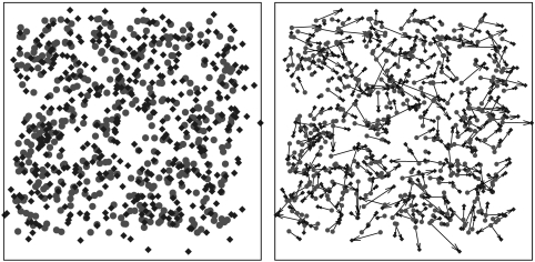
The level of difficulty soars as Λ increases: many sets of trajectories, i.e., many mappings among particles in successive images, have comparable likelihoods, see Fig. 1. The dynamics of the particles ought to be described by an explicit model, which generally features unknown parameters. The model defines a probability distribution over the space of all possible assignments. Contrary to the small Λ case, the probability distribution is not necessarily dominated by a unique assignment. Notwithstanding this uncertainty on the trajectories, it is expected that useful information might still be extracted if the number of tracked particles is sufficiently large. The difficulty is that all possible assignments must be considered: restricting to the most probable assignment (MPA) generally leads to biased inferences (see the sequel). Reliable inference requires summing over all possible assignments with their appropriate weights. Problems with large Λ occur in practice; e.g., even with state-of-the-art cameras, particles in turbulent flow (11) and birds in flocks (1) often feature ambiguities in the reconstruction of particles’ trajectories. Developing systematic methods to tackle these cases constitutes our scope here.

Fig. 1.

A concrete example of particle tracking, with N = 400 particles moving from their original positions (red circles) to new ones (blue diamonds). (Left) Two consecutive images are superimposed to facilitate comparison of the successive positions. Particles are transported by a turbulent fluid flow with local stretching, shear, vorticity and diffusivity parameters a^∗ = 0.28, b^∗ = 0.54, c^∗ = 0.24, and κ^∗ = 1.05 (see Eq. 9). We focus on turbulent transport because of the challenges it poses, yet the methods we develop are quite general. (Right) Actual motion of each particle. Evidently, the simple criterion of particle proximity fails to pick the actual trajectories, and the mapping of the particles between the two images is intrinsically uncertain. Nevertheless, the inference algorithms described here rapidly yield excellent predictions (a = 0.32, b = 0.55, c = 0.19, and κ = 1.00) for the parameters of the flow.

The plan of the paper is as follows. First, we formulate the problem of particle tracking in terms of a graphical model. We then show that an exact and rapid algorithm for summing over all possible assignments is unlikely to become available, as such an algorithm could equivalently compute the permanent of a nonnegative matrix, a problem that is well-known to be #P-complete (12). An approximate message-passing belief propagation (BP) algorithm (13–15) is then introduced, employed, and tested. We also introduce a simplified model where analytical results and a quantitative sense of the BP approximations are obtained. The Results section presents numerical simulations comparing results of BP and the inference based on the MPA. For the sake of concreteness, we consider the case of particles passively transported by a turbulent flow, but the methods are quite general and can be applied to other situations as well.

Models

Tracking of Particles as a Graphical Model.

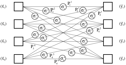
Graphical models provide a framework for inference and learning problems widespread in machine learning, bioinformatics, statistical physics, combinatorial optimization, and error-correction (13, 14, 16). The assignment problem involved in the tracking of particles is conveniently recast as a weighted complete bipartite graph (see Fig. 2). Nodes are associated with the N particles in each of two successive images, their positions being denoted x_i and y^j, respectively. These 2N position vectors (i, j = 1,…,N) constitute the experimental data provided. We suppose that a model for the dynamics of the particles is available and features a set of unknown parameters θ. Edges between nodes of the bipartite graph are weighted according to the likelihood that, according to this model, a particle moves from the initial position x_i to the final position y^j. Specifically, the formula for the likelihood of an assignment among (noninteracting) particles in two images reads as follows:

[1]

The Boolean variable indicates whether the particles i and j are matched () or not (). The set of the N² variables is denoted by {σ}. The constraint function , involving Kronecker δ functions, enforces the conditions for a perfect matching, i.e., a one-to-one correspondence between the particles in the two images. [Situations where the number of particles in the two images can differ and/or where the positions of the particles are uncertain are accommodated within the same formalism presented in the sequel (SI Appendix).] The quantity is the transition probability that a particle at position x_i travels to y_j in the time Δ between images. The transition probabilities carry all of the information about the model for the dynamics of the particles.

Fig. 2.

The complete bipartite graph for the tracking problem. Nodes (squares) denote particles in two consecutive images. Edges carry weights (the likelihood that a particle travels from the initial position x_i to the final position y^j) and Boolean variables [indicating whether the nodes i and j in the two images correspond to each other (σ = 1) or not (σ = 0]. Conflicts arise from the constraint that a valid assignment is a one-to-one mapping of the particles in the two images [expressed by the constraint C({σ}) in Eq. 1].

The tracking inference problem that we address here is to provide fast and reliable estimates of the model’s unknown parameters θ, which enter the likelihood of the trajectories via [Eq. 1].

The simplest method to infer the unknown parameters θ is first to identify for any θ the MPA, i.e., a configuration {σ} satisfying the constraint C({σ}) = 1 and having the highest likelihood [1], and then to maximize the resulting likelihood with respect to θ. Exact polynomial algorithms (8, 9) solve the first MPA task. The surprising remark recently made in refs. 10 and 17 is that the actual exact algorithm can be reformulated as a message-passing BP scheme. (Surprise stems from the fact that BP usually differs from the exact solution of a problem if loops are present in its graph.)

It is, however, expected—and confirmed by results described shortly—that the MPA provides reliable inferences only for small enough values of the stiffness parameter Λ defined in the Introduction. As Λ increases, assignment-dependent entropic factors become important, and MPA inferences deviate from the actual values of the parameters θ. This deviation is understandable because the Bayesian probability distribution for the parameters, assuming uniform prior probability for the assignments, involves the full likelihood [1] marginalized over all possible assignments:

[2]

As the stiffness parameter Λ increases, many assignments become likely and the sum [2] is not dominated by the MPA.

Summing Over All Possible Trajectories.

In the vast majority of cases, no exact algorithm is available to sum over all possible states of a graphical model. Expression 2 is no exception, as it can also be seen as a sum over all possible permutations of the lower indices i into the upper indices j. It is then recognized that computing the likelihood Z (also known as partition function in statistical physics) is equivalent to computing the permanent of the matrix , a well-known #P-complete problem (12). However, the matrix in our sum [2] is nonnegative and the permanent of nonnegative matrices was discovered to be solvable by a fully polynomial randomized approximation scheme (FPRAS) (18). The complexity of the original FPRAS algorithm is O(N¹¹). We significantly accelerated [to O(N³)] and simplified the original Markov Chain Monte Carlo (MCMC) algorithm of (18) without observable deterioration of its quality (see SI Appendix). In Results, we use this simplified version to assess the accuracy of our BP approximation while in the SI Appendix we compare performance of BP to the MCMC scheme.

Among the possible approximations to compute the permanent of a matrix, belief propagation has a special status because of its aforementioned exactness for the MPA problem (10). Moreover, the BP algorithm is very fast, scaling as O(N²) in its basic form and linearly if, for each particle, only a limited number of nearby particles is considered. We shall therefore pursue the development of BP to approximate the sum in [2] and then assess its validity through numerical simulations and the simplified “random distance” model discussed shortly.

The starting point of the BP approach is the remark that the convex Kullback-Leibler functional

[3]

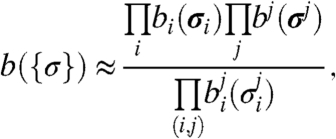
has a unique minimum at [under the normalization condition ], where is defined in [1] and Z in [2]. The corresponding value of the functional is the log-likelihood (free energy), . This remark constitutes the basis for variational methods (see ref. 14), where the minimum of the functional is sought in a restricted class of functions. BP (and the corresponding approximation for the free energy, named in ref. 15 after Hans Bethe), involves an ansatz of the form

[4]

where each vector can be any of the N possible vectors (0,⋯,0,1,0,⋯,0) having exactly one nonzero entry, and σ^j is defined analogously. This ansatz is motivated by the fact that the probability distribution on a graph with a tree structure, i.e., without loops, takes exactly the form [4]. The quantities b_i, b^j, and are called “beliefs.” In the absence of loops, represents the probability distribution for the single Boolean variable , and b_i represents the joint probability distribution of the components of σ_i, which appear in a constraint. Without loops, the beliefs automatically satisfy the conditions of marginalization, viz., , where the sum is performed over all possible values of the vector σ_i having the specified value of its component .

In the presence of loops, the expression [4] is no longer exact, and the marginalization conditions must be imposed as additional constraints. The important point demonstrated in ref. 15 is that minimizing the functional [3] for the class of functions [4] (under the marginalization and the normalization conditions) yields the message-passing formulation of BP, which was heuristically introduced by Gallager for decoding of sparse codes (19).

Most commonly, the BP equations are formulated as an iterative message-passing scheme (14, 16), where the message (respectively, ) is sent from particle i in the first (second) image to particle j in the second (first) image. In the case of the matching problem, the messages are determined by solving the following equations:

[5]

The “inverse temperature” β can be set to unity, but it is usefully retained to show that the limit β → ∞ yields the exact solution for the MPA problem (10).

To solve the BP Eqs. 5, the messages are randomly initialized and iteratively updated in order to find a fixed point of the message-passing Eqs. 5. The Bethe free energy then reads

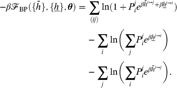[6]

The Bethe free energy , evaluated at the fixed point of the BP Eqs. 5, provides an estimate of the exact log-likelihood - ln Z(θ) defined through [2]. Because the most likely set of parameters θ minimizes - ln Z(θ), we seek parameters that minimize the estimated free energy. We perform this minimization using Newton’s method in combination with message-passing: after each Newton step, we update the messages according to [5] and the current set of parameters θ. As this combined update takes N² steps and the number of combined steps which led to convergence is N-independent, the running time scales as O(N²). Note that the running time can be further reduced to O(N) neglecting the contribution of edges with very small probability , i.e. diluting the fully connected bipartite graph.

A Simplified Model to Understanding the BP Approximation.

The BP approximation is exact only if the underlying graph is a tree, which is not the case for our fully connected bipartite graph in Fig. 2. In Results, we empirically assess the validity of the BP approximation through numerical simulations. To supplement the numerical evidence, we introduce here a simplified “random distance” model for which analytical results can be obtained and used to understand the nature of the BP approximation.

The “random distance” model is defined as follows. First, we decouple the N² distances between particles i and j by assuming that they are independent among each other. We then assume that one permutation π^∗ of the lower indices i into the upper indices j has a special status, while all other distances are drawn independently at random from a given distribution. Namely, the N distances ’s are distributed as a Gaussian (restricted to positive values) with variance κ^∗ = O(1). For each of the other N(N - 1) pairs (i,j), the distances are independent random variables drawn uniformly in the interval (0,N). Units of length are chosen so that the typical interparticle distance is set to unity. Note that any distribution of for with a vanishing derivative at the origin would give the same solution. Indeed, the crucial property is that, for each particle i, the number of distances that are comparable with the diffusion length scale is O(1).

The interest of a special permutation π^∗ is that we can inquire about: learning κ^∗ if π^∗ is supposed unknown; the relevance of entropic factors for the partition function; and the status of the BP approximation. The same questions arise for [2] in the original problem. Note that if there were no special permutation, then we would obtain the random link model considered in refs. –22. Our “random distance” model can be solved exactly in the thermodynamic limit using the replica method, as in refs. 20, 21, or using the cavity method, as in ref. 22. The main result (see SI Appendix) is that the BP expression of the free energy for the “random distance” model is exact in the limit N → ∞, despite the short loops in the graph of the model. The argument to prove this result goes as follows: (a) the contribution to the partition function [2] from those permutations of the j indices that contain distances larger than O(1) is negligible; (b) as each node has only a fraction O(1) of its N distances being O(1), the underlying graph is effectively sparse; (c) because sparse graphs are locally tree-like and correlations in the matching problem decay very fast on trees, it follows that the BP approximation is exact in the thermodynamic limit. We have formalized these statements within the replica and cavity methods [and rigorous local weak convergence methods are probably also applicable, as for the random link model (23)].

The asymptotic exactness found in the “random distance” model means that errors made by BP are caused by correlations among the interparticle distances. In a smooth flow (see the sequel) particles close to each other in the first image will also be near each other in the second image; moreover, the four distances among the two positions in the first image and the two positions in the second will also be small, or more generally correlated. This effect is more important in lower dimensions. Indeed, BP inferences turn out to be better in the three-dimensional (3D) case than in 2D and rather inaccurate in 1D (with maximum relative error about 60%).

Our replica calculations also show that the “random distance” model presents an interesting phase transition at the diffusivity κ_c ≈ 0.174. For κ^∗ < κ_c, the MPA π_MPA is identical to the special one π^∗ with high probability, whereas for κ^∗ > κ_c the overlap (defined via the Hamming distance) between the most likely assignment π_MPA and the special one π^∗ is extensive, i.e., O(N). The comparison with the finite-dimensional case is discussed in Results.

Results

Our analysis has been quite general so far. To concretely assess the validity of BP, it is now necessary to specify the model appearing in the likelihood [1], namely, the probability for the transition from position x_i to y^j in the image acquisition time Δ. We decided to focus on the tracking of particles in turbulent flow for three reasons. First, the problem is highly relevant as an important part of modern experiments in fluid dynamics is based on the tracking of particles either in simple (4–6) or complex (24) flows. Second, all the algorithms used so far for reconstructing the flow from images of multiple particles have ignored the probabilistic structure of the possible assignments. As discussed in the review (11), the general approach is to search for a single matching. Criteria based on proximity and/or minimal acceleration identify for each particle its “best” mapping in the successive time-image. Conflicts where two or more particles in the first image are assigned to the same particle in the second image are resolved by various heuristics. The simplest option is to give up on those situations where a conflict arises; the most elaborate solution is to compute the assignment with the minimal cost in terms of proximity or acceleration. The bottom line is that one is always left with a single assignment, which leads to predictions that are effective at low density of the particles but rapidly degrade as their density increases (11). Third, the laws of motion of the particles are well-known. Indeed, if particles are sufficiently small and chosen of appropriate (mass) density, their effect on the flow is negligible and they are transported almost passively. The (number) density of particles is usually rather high and a single snapshot contains a large number thereof. The reason is that the smallest scales of the flow ought to be resolved. Furthermore, turbulence is quite effective in rapidly transporting particles so that the acquisition time between consecutive snapshots should be kept small. Modern cameras have impressive resolutions, on the order of tens of thousands of frames per second. The flow of information is huge: ∼Gigabit/s to monitor a two-dimensional slice of a (10 cm)³ experimental cell with a pixel size of 0.1 mm and exposure time of 1 ms. This high rate makes it impossible to process data on the fly unless efficient algorithms are developed.

Tracking of Particles in a Turbulent Flow.

The likelihood in Eq. 1 for the transport of particles in turbulent flow is obtained as follows. Tracked particles are supposed to be at reciprocal distances smaller than the viscous scale of the flow. It follows (see ref. 25 for a review) that the position r_i(t) of the ith particle evolves according to the Lagrangian stochastic equations: . Positions are measured with respect to a reference point and is the tensor of the velocity derivatives. In a two-dimensional incompressible flow, a = s_xx = -s_yy is the rate of stretching, b = (s_xy + s_yx)/2 is the shear, and c = (s_xy - s_yx)/2 is the vorticity. The stochastic term ξ_i(t) is the zero-mean Gaussian Langevin noise, describing molecular diffusivity, defined by its correlation function: 〈(ξ_i)_α(t₁)(ξ_j)_β(t₂)〉 = 2κδ_ijδ_αβδ(t₁ - t₂). The Greek indices refer to space components. The transition probability corresponding to the previous transport process is Gaussian:

[7]

[8]

[9]

where * and Δ denotes the image acquisition time. The general problem of estimating the unknown parameters θ now takes the special form of inferring the components of the tensor and the diffusivity κ.

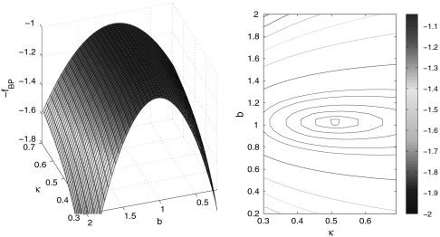
We tested the BP inference method on numerically simulated data. To compare different system sizes, we placed the N particles at random in a d-dimensional box of size L = N^1/d, i.e., the average density equals unity. Particles are then displaced independently following the probabilistic distribution [7] with a set of parameters a^∗N^-1/d, b^∗N^-1/d, c^∗N^-1/d, κ^∗. The timescale was chosen as the acquisition time Δ = 1 and the parameters a, b, c of the flow were rescaled by N^-1/d, so that the particle displacements in the acquisition time are O(1) for all choices of N. Fig. 3 shows the BP free energy [6] as a function of the shear b and the diffusivity κ for N = 200 particles. The curvature around the minimum of the exact free energy is inversely related to the statistical error in the estimation of the parameters. Fig. 3 clearly shows that the most problematic parameter is the diffusivity κ, as confirmed by all of the numerical simulations we performed.

Fig. 3.

A realization of a two-dimensional flow with a^∗ = b^∗ = c^∗ = 1, κ^∗ = 0.5, and N = 200 particles. (Left) The BP Bethe free energy as a function of the diffusivity κ and the shear b, where every point is obtained by minimizing with respect to the stretching a and the vorticity c of the flow. (Right) The same free energy in a contour plot, showing the maximum close to b = 1 and κ = 0.5. The maximum is achieved for , b_BP = 1.026(1), c_BP = 0.945(1), and κ_BP = 0.509(1), where the parentheses indicates numerical error on the third digit.

In the next three figures, we concentrate on the purely diffusive regime (where a^∗ = b^∗ = c^∗ = 0); subsequently, we return to the general case. Note that light scattering experiments provide an established measurement method for biological systems (26–29). The technique is not commonly used in fluid dynamics experiments because the dispersion of the particles is much faster and the typical illumination level is too weak.

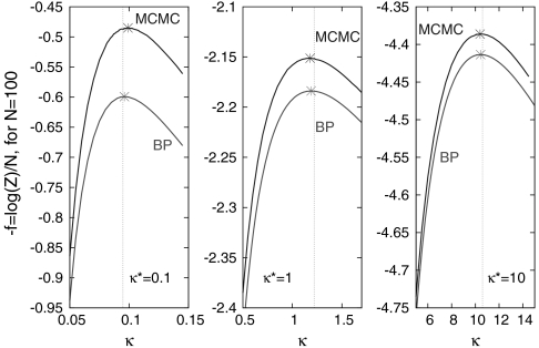
In Fig. 4 we compare the BP results with results from the fully polynomial randomized approximation scheme based on the MCMC method. As computed by MCMC (which is guaranteed to be a FPRAS), the maximum of Z(κ) coincides with the true value κ^∗. From the large deviation theory interpretation of , it follows that the statistical error of the estimation of κ is . Fig. 4 confirms the expectation that the curvature at the minimum of the free energy decreases with the diffusivity constant κ.

Fig. 4.

The BP estimate of the log-likelihood and the Monte Carlo Markov Chain estimate plotted vs. the diffusivity κ with κ^∗ = 0.1, 1, 10 for N = 100 particles diffusing in 3D. Although the BP log-likelihood is significantly lower than the MCMC one, the estimate of the diffusivity is extremely good. The vertical lines mark the diffusivity computed based on the knowledge of the actual displacements. The BP algorithm compares favorably in estimation of the maximum with the basically exact Markov Chain Monte Carlo algorithm, while being far superior in speed (for details on speed comparison see SI Appendix).

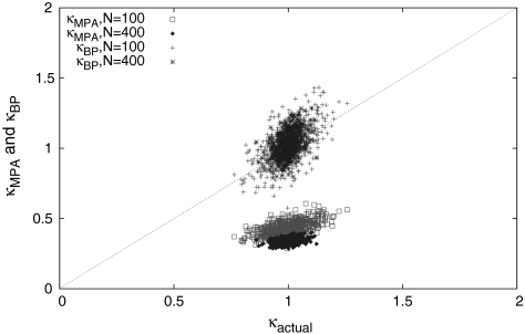
In Fig. 5 we compare the estimates of the diffusivity using BP (κ_BP) and using MPA (κ_MPA). The actual value κ_actual (respectively, the MPA estimate κ_MPA) is computed as the mean-square displacement of the particles on the actual (resp., the most probable) trajectories of the particles. The key conclusion to be drawn from Fig. 5 is that MPA largely underestimates the diffusivity, whereas the BP method is accurate.

Fig. 5.

Scatter plot of the diffusivity estimated by BP and by MPA vs. the actual value of the diffusivity. Diffusion takes place in 3D, with displacements generated using κ^∗ = 1. The actual value of the diffusivity κ_actual is computed from the actual trajectories and is subject to statistical fluctuations. The number of tracked particles is N = 100 (light gray) and N = 400 (dark gray) using 1,000 measurements. The BP predictions correspond to the maximum of the log-likelihood, as approximated by the Bethe free energy [6] discussed in the text. Note the strong underestimation of the MPA estimate, to be contrasted with the cloud of BP predictions centered around the correct value of κ^∗.

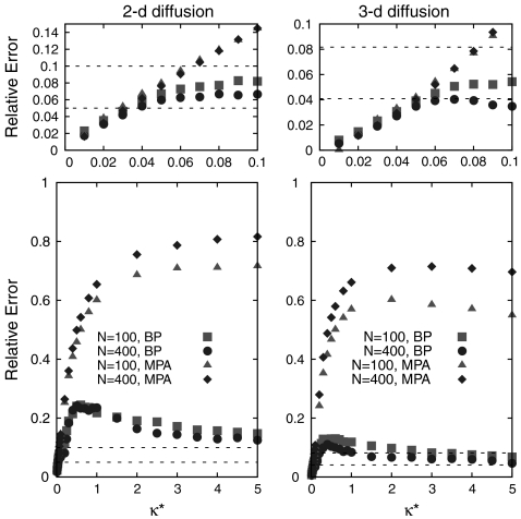
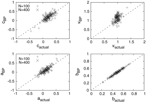
Fig. 6 gives a quantitative sense of the BP accuracy as a function of the diffusivity. The upshot of the curves is that MPA gives accurate estimates only at extremely low diffusivities. Conversely, as the diffusivity increases and the overlap among possible assignments becomes important, the quality of MPA predictions degrades very rapidly. Results from a similar study for 2D flows is presented in Fig. 7; vectorial parameters are again found to be computed efficiently by the BP method.

Fig. 6.

The relative error in the estimates of the diffusivity over K measurements vs. the actual value of the diffusivity κ^∗. Circles and squares refer to BP while triangles and lozenges refer to the MPA. κ_actual is the actual value of the mean-square displacement of the particles, i.e., it includes fluctuations around κ^∗ due to the finite number N of particles. The data are averaged over 1,000 (for N = 100) and 250 (for N = 400) realizations and compared to the relative statistical error (dashed horizontal lines). The case of 2D diffusion is shown on the left, and the 3D case is on the right. The top figures are zooms into the low diffusivity region.

Fig. 7.

Scatter plot of the parameter estimations using the BP method in the case of a 2D incompressible flow with the rate of stretching a^∗ = 0.1, the shear b^∗ = 0.5, the vorticity c^∗ = 0.2, and the diffusivity κ^∗ = 1. Light (dark) points refer to the case of a number of tracked particles N = 100 (N = 400) and the number of measurements is 50.

Finally, Fig. 6 (Top) indicates that the phase transition in the exactness of the optimal assignment, which was previously found for our “random distance” model, is smeared out in the finite-dimensional case (or it happens only at κ < 0.01). This effect is traced to the fact that, in a finite dimension, there are always several pairs of particles at distance o(1) that get confused with the diffusion [when κ^∗ = O(1)]. It follows that the probability for π_MPA = π^∗ is always smaller than unity.

Discussion

The message-passing algorithms discussed here were shown to ensure efficient, distributed, and accurate learning of the parameters governing the stochastic map between two consecutive images recording the positions of many identical particles. The general method was illustrated in a model relevant for the tracking of particles in fluid dynamics. It was shown that parameters of the flow transporting the particles could be efficiently and reliably predicted even in situations where a strong uncertainty in the particles’ trajectories is present.

We introduced and compared two techniques to approximate the likelihood that the dynamics of the particles is compatible with the displacements observed in the experimental snapshots. The first is based on finding the most probable trajectories of the particles between the times of the two images. The second corresponds to evaluating the probabilistically weighted sum over all possible trajectories. The latter is a #P-complete problem and its solution is approximated by belief propagation, as implemented via a message-passing algorithm. BP was shown to become exact for the simplified “random distance” model we introduced here. In general, the effect of loops in the graphical model for the tracking problem remains nonzero even in the thermodynamic limit of a large number of tracked particles. Preliminary analysis of the loop corrections to BP did not display any immediately visible structure, yet detailed analysis of this point is left for future work. Another interesting direction is the development of learning algorithms (both MCMC and message-passing) specifically designed to provide estimations of appropriate observables, e.g. the sum of the square of the distances traveled by the particles, whence the parameters of the dynamics, e.g. the diffusivity, can be estimated. This could lead to further reductions in the computational time and it will be of interest to test whether the superiority in speed we found here for BP as compared to the FPRAS Monte Carlo scheme (see SI Appendix) still holds. The price of a single observable is that the log-likelihood curves in Fig. 4 offer more complete information, namely, a systematic way to gauge the error bars on the inferred parameters.

The algorithms presented here can be carried over to the tracking of other types of “particles,” e.g., those of biological interest. Motile bacteria in colonies, eukaryotic cells, or fluorescent biomolecules provide relevant examples. As it was stressed here, our methods are poised to deal with dense conditions where a strong overlap among the various particles’ trajectories are present. An additional use of the techniques introduced here is to compare different models of transport, e.g., purely diffusive, directed, active, etc. The Bethe expression given by the BP approximation can be taken as an approximation for the log-likelihood of the various models, which are then compared by standard model selection tests. The validity of the various models postulated for the dynamics of the tracked objects can thus be quantitatively compared.

Our main conclusion is that the BP method gives accurate results and its computational burden is comparable to identifying the most probable trajectories. The accuracy of BP was shown to compare extremely well with exact results and to improve rapidly as the dimensionality of the problem increases. The BP-based technique allows generalization to reconstruction of a multiscale flow from particle images in two sequential snapshots. BP can also be adapted to the case where trajectories of the particles are reconstructed from their positions in several (> 2) images (see SI Appendix). In conclusion, the formulation of particle tracking as an inference problem permits tackling it systematically and introducing message-passing methods that are highly effective in diverse applications.

References

- 1.Ballerini M, et al. Interaction ruling animal collective behavior depends on topological rather than metric distance: Evidence from a field study. Proc Natl Acad Sci USA. 2008;105:1232–1237. doi: 10.1073/pnas.0711437105. [DOI] [PMC free article] [PubMed] [Google Scholar]
- 2.Keller PJ, Schmidt AD, Wittbrodt J, Stelzer EHK. Reconstruction of zebrafish early embryonic development by scanned light sheet microscopy. Science. 2008;322:1065–1069. doi: 10.1126/science.1162493. [DOI] [PubMed] [Google Scholar]
- 3.Saxton MJ. Single-particle tracking: Connecting the dots. Nat Meth. 2008;5:671–672. doi: 10.1038/nmeth0808-671. [DOI] [PubMed] [Google Scholar]
- 4.La Porta A, Voth GA, Crawford AM, Alexander J, Bodenschatz E. Fluid particle accelerations in fully developed turbulence. Nature. 2001;409:1017–1019. doi: 10.1038/35059027. [DOI] [PubMed] [Google Scholar]
- 5.Mordant N, Metz P, Michel O, Pinton JF. Measurement of Lagrangian velocity in fully developed turbulence. Phys Rev Lett. 2001;87:214501. doi: 10.1103/PhysRevLett.87.214501. [DOI] [PubMed] [Google Scholar]
- 6.Adrian RJ. Particle-imaging techniques from experimental fluid mechanics. Ann Rev Fluid Mech. 1991;23:261–304. [Google Scholar]
- 7.Masson JB, et al. Inferring maps of forces inside cell membrane microdomains. Phys Rev Lett. 2009;102:048103. doi: 10.1103/PhysRevLett.102.048103. [DOI] [PubMed] [Google Scholar]
- 8.Kuhn HW. The Hungarian method for the assignment problem. Nav Res Logist Q. 1955;2:83–97. [Google Scholar]
- 9.Bertsekas DP. Auction algorithms for network flow problems: A tutorial introduction. Comput Optim Appl. 1992;1:7–66. [Google Scholar]
- 10.Bayati M, Shah D, Sharma M. Max-product for maximum weight matching: Convergence, correctness and LP duality. IEEE T Inform Theory. 2008;54:1241–1251. [Google Scholar]
- 11.Ouelette NT, Xu H, Bodenschatz E. A quantitative study of three-dimensional Lagrangian Tracking Algorithm. Exp Fluids. 2006;40:301–313. [Google Scholar]
- 12.Valiant LG. The complexity of computing the permanent. Theor Comput Sc. 1979;8:189–201. [Google Scholar]
- 13.Pearl J. In: Probabilistic Reasoning in Intelligent Systems: Networks of Plausible Inference. Morgan Kaufmann., editor. San Francisco, CA: Morgan Kaufmann; 1988. [Google Scholar]
- 14.MacKay DJC. Information Theory, Inference, and Learning Algorithms. New York: Cambridge Univ Press; 2003. [Google Scholar]
- 15.Yedidia JS, Freeman WT, Weiss Y. Constructing free-energy approximations and generalized belief propagation algorithms. IEEE T Inform Theory. 2005;51:2282–2312. [Google Scholar]
- 16.Mezard M, Montanari A. Information, Physics and Computation. New York: Oxford Univ Press; 2009. [Google Scholar]
- 17.Chertkov M. Exactness of belief propagation for some graphical models with loops. J Stat Mech-Theory E. 2008 10.1088/1742-5468/2008/10/P10016. [Google Scholar]
- 18.Jerrum M, Sinclair A, Vigoda E. A polynomial-time approximation algorithm for the permanent of a matrix with nonnegative entries. J ACM. 2004;51:671–697. [Google Scholar]
- 19.Gallager RG. Low Density Parity Check Codes. Cambridge, MA: MIT Press; 1963. [Google Scholar]
- 20.Mezard M, Parisi G. Replicas and optimization. J Phys-Paris. 1985;46:771–778. [Google Scholar]
- 21.Mezard M, Parisi G. Mean-field equations for the matching and the traveling salesman problems. Europhys Lett. 1986;2:913–918. [Google Scholar]
- 22.Martin OC, Mezard M, Rivoire O. Frozen glass phase in the multi-index matching problem. Phys Rev Lett. 2004;93:217205. doi: 10.1103/PhysRevLett.93.217205. [DOI] [PubMed] [Google Scholar]
- 23.Aldous DJ. The ζ(2) limit in the random assignment problem. Random Struct Algor. 2001;18:381–418. [Google Scholar]
- 24.Ouellette NT, Xu HT, Bodenschatz E. Bulk turbulence in dilute polymer solutions. J Fluid Mech. 2009;629:375–385. [Google Scholar]
- 25.Falkovich G, Gawedzki K, Vergassola M. Particles and fields in fluid turbulence. Rev Mod Phys. 2001;73:913–975. [Google Scholar]
- 26.Magde D, Webb WW, Elson E. Thermodynamic fluctuations in a reacting system—Measurement by fluorescence correlation spectroscopy. Phys Rev Lett. 1972;29:705–708. [Google Scholar]
- 27.Elson EL, Magde D. Fluorescence correlation spectroscopy. 1. Conceptual basis and theory. Biopolymers. 1974;13:1–27. doi: 10.1002/bip.1974.360130103. [DOI] [PubMed] [Google Scholar]
- 28.Magde D, Elson EL, Webb WW. Fluorescence correlation spectroscopy. 2. Experimental realization. Biopolymers. 1974;13:29–61. doi: 10.1002/bip.1974.360130103. [DOI] [PubMed] [Google Scholar]
- 29.Rigler R, Mets U, Widengren J, Kask P. Fluorescence correlation spectroscopy with high count rate and low background: Analysis of translational diffusion. Eur Biophys J. 1993;22:169–175. [Google Scholar]
Associated Data
This section collects any data citations, data availability statements, or supplementary materials included in this article.