Retinal Nerve Fiber Layer Thickness Measurement Comparability between Time Domain Optical Coherence Tomography (OCT) and Spectral Domain OCT

The authors developed an algorithm for measurement comparability between time domain optical coherence tomography (TD-OCT) and spectral domain OCT (SD-OCT). This method may facilitate bridging the gap between measurements obtained by the different generations of OCT technology.

Abstract

Purpose.

Time domain optical coherence tomography (TD-OCT) has been used commonly in clinical practice, producing a large inventory of circular scan data for retinal nerve fiber layer (RNFL) assessment. Spectral domain (SD)-OCT produces three-dimensional (3-D) data volumes. The purpose of this study was to create a robust technique that makes TD-OCT circular scan RNFL thickness measurements comparable with those from 3-D SD-OCT volumes.

Methods.

Eleven eyes of 11 healthy subjects and 7 eyes of 7 subjects with glaucoma were enrolled. Each eye was scanned with one centered and eight displaced TD-OCT scanning circles. One 3-D SD-OCT cube scan was obtained at the same visit. The matching location of the TD-OCT scanning circle was automatically detected within the corresponding 3-D SD-OCT scan. Algorithm performance was assessed by estimating the difference between the detected scanning circle location on 3-D SD-OCT volume and the TD-OCT circle location. Global and sectoral RNFL thickness measurement errors between the two devices were also compared.

Results.

The difference (95% confidence interval) in scanning circle center locations between TD- and SD-OCT was 2.3 (1.5–3.2) pixels (69.0 [45.0–96.0] μm on the retina) for healthy eyes and 3.1 (2.0–4.1) pixels (93.0 [60.0–123.0] μm on the retina) for glaucomatous eyes. The absolute RNFL thickness measurement difference was significantly smaller with the matched scanning circle.

Conclusions.

Scan location matching may bridge the gap in RNFL thickness measurements between TD-OCT circular scan data and 3-D SD-OCT scan data, providing follow-up comparability across the two generations of OCTs.

Optical coherence tomography (OCT) provides noncontact and noninvasive retinal nerve fiber layer (RNFL) thickness measurements and has become an essential clinical measure for objective glaucoma assessment.^1–4 RNFL thickness is measured on a cross-sectional retinal image sampled along a 3.4-mm diameter circle centered on the optic nerve head (ONH). The operator manually places the time-domain (TD)-OCT circular scan around the ONH, introducing measurement variability and impeding the accuracy and reliability of long-term follow-up (Fig. 1A).^5,6 In addition, immeasurable scattering of the sampling locations in the vicinity of the planned circular scanning path, due to eye movements during scanning, further complicates the accurate RNFL assessment (Fig. 1B).

Figure 1.

Limitations of the 3.4-mm-diameter circle scan of the TD-OCT. The scan circle can be different from scan to scan because scan circle placement is operator dependent (A), and sampling points can be scattered along 3.4-mm-diameter circle due to eye motion (B).

Recently, spectral domain OCT (SD-OCT) technology has been introduced providing faster scanning (up to 100×) and finer axial resolution (up to 2×) compared with TD-OCT.⁷ Faster scanning allows high-resolution, three-dimensional (3-D) volume sampling by raster scanning in the region of interest. Involving the summation of the back-scattered signal at each transverse point of a retinal raster scan, 3-D SD-OCT data can be visualized as an en face image of the retina. The en face retinal image is also known as an OCT fundus image (Fig. 2A).⁸ The OCT fundus image permits the detection of eye movements during scanning by checking for discontinuities in retinal blood vessels. It can also be used to create a virtual OCT cross-sectional (B-scan) image along any sampling line (curved or straight; Fig. 2B, white circle). Therefore, near perfect registration of a virtually sampled B-scan image can be achieved.

Figure 2.

3-D SD-OCT data visualization. By summing the reflectivity data in z-direction (A, left), the OCT fundus (en face) image is generated (A, right). On the OCT fundus image, one can specify any resampling path (e.g., circular scanning path; B, left) so that a virtual resampled OCT cross-sectional image can be generated (B, right).

A major limitation in the clinical implementation of SD-OCT is the incomparability of RNFL thickness data between the two generations of the OCT technology. Because of the differences in the signal characteristics and the RNFL border segmentation algorithms between the two generations, measured RNFL thickness is not directly comparable.^9–11 To overcome this difference, a calibration equation needs to be established between the generations. In addition, the manual nature of the scan registration with TD-OCT requires scan registration to be matched after calibration to reduce measurement variability. This reduction in variability is especially important when trying to detect glaucoma progression, which can appear as localized minor changes. Since 3-D SD-OCT volume data allow us to virtually sample along any arbitrary line, detection of the TD-OCT scan location within the corresponding 3-D SD-OCT data may reduce measurement variability between the two generations.

We hypothesized that an automated detection of the TD-OCT circular scan registration location within the corresponding 3-D SD-OCT can be achieved by using OCT image data without using any external reference information, such as the video fundus image. The purpose of this study was to develop an automated system for such scan location matching between TD- and SD-OCT and to test its performance in terms of accuracy of the matched scanning circle location as well as the RNFL thickness measurements.

Methods

Eleven eyes of 11 healthy subjects and 7 eyes of 7 subjects with glaucoma from the University of Pittsburgh Medical Center Eye Center were enrolled. The University of Pittsburgh Institutional Review Board and ethics committee approval were obtained for the study, and informed consent was obtained from all subjects. The study protocol adhered to the tenets of the Declaration of Helsinki and was conducted in compliance with the Health Insurance Portability and Accountability Act.

Clinical Diagnosis

Inclusion criteria were best corrected visual acuity of 20/40 or better, refractive error within ±6.0 D, and no media opacities that might interfere with fundus imaging. Subjects were excluded if they were using medications known to affect retinal thickness or if they had systemic diseases that might affect the retina or visual field. Subjects were also excluded if they had any previous intraocular surgeries other than uneventful cataract extraction. One randomly selected eye was included if both eyes were eligible in the same subject.

Healthy eyes had normal findings in a comprehensive ocular examination and an automated perimetry glaucoma hemifield test (GHT) within normal limits (Humphrey Visual Field Analyzer, HVF IIi; Carl Zeiss Meditec, Inc. [CZMI], Dublin, CA). Glaucomatous eyes showed both glaucomatous optic neuropathy and GHT outside normal limits. Glaucomatous optic neuropathy was defined as general or focal neuroretinal rim thinning, disc hemorrhage, or intereye cup/disc ratio asymmetry >0.2.

Image Acquisition

The peripapillary region was scanned on all eyes using conventional TD-OCT (Stratus OCT; CZMI) and SD-OCT (Cirrus HD-OCT; CZMI) at a single visit. All scans were performed through dilated pupils.

Stratus OCT.

Circular scans centered around the ONH were obtained using the circle scan pattern, which was a single 3.4-mm diameter circular scan with 256 × 1024 samplings acquired in 0.64 second. Nine circle scans were obtained from each eye in a single session by one operator (MLG). Each of the nine scans had its scanning circle manually centered differently (Fig. 3), starting with the circle manually centered on the ONH followed by eight different manual displacements so that each circle had a clearly visible displacement without touching the ONH margin. Images with signal strength (SS) <6 were discarded as poor-quality images as the manufacturer recommends. RNFL thickness was measured using the Stratus OCT system software version 5.0. Segmentation failure was defined as obvious deviation of the segmented inner and/or outer RNFL borders from the subjectively perceived borders. Consecutive 5% or cumulative 10% segmentation failure within a given image was considered to be poor analysis quality and discarded.

Figure 3.

Illustration of TD-OCT circle scans in nine different locations per eye.

Cirrus HD-OCT.

A single optic disc cube 200 × 200 scan was obtained from each eye. This isotropic (equal A-scan spacing in x, y plane) raster scan contained 200 × 200 × 1024 samplings of a 6 × 6 × 2-mm volume manually centered on the ONH and was acquired in 1.48 seconds. Images with SS <8 were discarded as poor-quality images, as the manufacturer recommends. This cutoff differs from that of TD-OCT because of inherent hardware and software differences between the two platforms. Inclusion also required that eye movements be less than the diameter of major vessels judged on OCT fundus images. The segmentation quality criteria for virtual OCT slices (or resampled images) from the Cirrus scans was the same as for the Stratus OCT scans with the additional criteria of >10% of frames labeled as analysis failure disqualified any scan.

Scan Location Matching Process

Every possible 3.4-mm circular resampling path contained within the physical boundaries of the 3-D SD-OCT scan was generated (Fig. 4). Along each circle, a virtual OCT cross-sectional image was resampled with 256 evenly distributed sampling points (A-scans). The spatially closest actual A-scan data within the 3-D volume were used for resampling arbitrary virtual location.

Figure 4.

Visualization of the resampling process. Resampling of the center boundary (light green square) was performed so that the virtual 3.4-mm-diameter circles did not go out of the sampled volume, to avoid missing data points. During the search of the matching resampling center, the algorithm iterates from the center point A through the center point B, pixel by pixel within the green square.

Each A-scan of the resampled scans was aligned to a corresponding A-scan in the TD-OCT circular scan. Similarity for each virtual scan was assessed by cross correlation, and generation of a 2-D similarity map, with correlation coefficient value ranging from 0 to 1 (Fig. 5). The location of the resampled scan with the highest correlation coefficient was automatically recorded as the most likely location of the center of the TD-OCT scan.

Figure 5.

Scan location matching sample: (A, B) Fundus video (A) and cross-sectional OCT (B) images of a TD-OCT circular scan; (C, D) OCT fundus (C) and virtually resampled cross-sectional OCT (D) images of a SD-OCT 3-D scan on the same eye; (E) Similarity map generated by computing correlation coefficients between TD-OCT data and virtually resampled data centered at each pixel within the resampling center boundary (color range correlation coefficient 0, dark blue, to 1, white); (F) Aligned matching virtually resampled image. Note that the locations of the vessel shadows nicely match up with TD-OCT image (dashed lines).

Similarity Assessment of the Matched Scan Location

Agreement between matched scan locations was assessed by measuring the distance between the center points of the TD-OCT and the matched virtual SD-OCT scans. Global and sectoral RNFL thickness measurements from these 2 OCT scans were also compared.

Distance between the Center Points.

Each TD-OCT video fundus image was manually registered with the corresponding SD-OCT fundus image by rotation, scaling, and translation, using major vessels as references (Fig. 6). The distance between the center points of the scan circles was measured on the composite image.

Figure 6.

Manual registration of TD-OCT video fundus image with SD-OCT fundus image: (A) SD-OCT fundus image; (B) TD-OCT video fundus image with circle scan location (blue); (C) matched scan location with virtual 3.4-mm circle on SD-OCT fundus image; (D) two fundus images, manually registered by rotating, scaling, and translation (green SD-OCT fundus image superimposed on yellow TD-OCT video fundus image), and the matched scan circle (white), imported to the registered image.

RNFL Thickness Measurements Comparison.

RNFL thickness, from the nine TD-OCT scans, was obtained using the Stratus OCT system software (version 5.0). SD-OCT RNFL thickness measurements were obtained using Cirrus HD-OCT the system software (ver. 3.0) at both the default ONH centered location and the matched scan location.

RNFL thickness measurements between TD-OCT and SD-OCT with the same eye are known to be different.^9–11 A calibration equation was computed to compensate for these systematic differences in RNFL thickness measurements between TD-OCT and SD-OCT. This computation was performed by using an independent group consisting of 48 eyes of 24 healthy subjects. All eyes satisfied the criteria for healthy eyes and were scanned both with TD- and SD-OCT at the same visit. The following calibration equation was modeled with estimating the bias components (α and β) in the RNFL thickness measurement between TD- and SD-OCT:

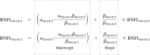where the ratio of the betas (β_TD-OCT and β_SD-OCT) adjusts for scale differences between the two devices (TD-OCT and SD-OCT), and the alphas (α_TD-OCT and α_SD-OCT) represent the bias intercepts in the statistical structural equation model (SEM), whereas the betas represent the regression slopes between the latent variables and the observed variables for each device and location.

Table 1 shows the estimated bias and the calibration equation components for both devices. When the ratio of the betas equals 1 and the differences between alphas equal 0, there is no bias. When the ratio of the betas equals 1 and the difference of the alphas is nonzero, there is a constant bias. When the ratio of the betas differs from one, there is a nonconstant bias (i.e., the bias changes with the measurement level).

Table 1.

The Estimated Bias and the Calibration Equation Components RNFL Thickness Measurements

Sector	Bias Estimation							Calibration Equation
	TD-OCT		SD-OCT		Ratio: βTD-OCT/βSD-OCT			On TD-OCT Scale		On SD-OCT Scale
	α	β	α	β	Lower	Est.	Upper	Intercept	Slope	Intercept	Slope
Global mean	2.51	1.00	−2.51	1.00	0.83	1.01	1.23	5.04	1.01	−4.99	0.99
Quadrant
Temporal	−5.52	1.14	4.46	0.88	0.92	1.30	1.90	−11.30	1.30	8.72	0.77
Superior	1.61	1.01	−1.64	0.99	0.81	1.03	1.30	3.29	1.03	−3.20	0.97
Nasal	6.52	0.95	−6.68	1.05	0.65	0.91	1.25	12.59	0.91	−13.87	1.10
Inferior	11.34	0.92	−12.14	1.09	0.72	0.85	0.99	21.65	0.85	−25.51	1.18
Clock hour
1	−18.79	1.21	14.92	0.83	0.79	1.47	2.06	−40.71	1.47	27.71	0.68
2	7.29	0.94	−7.59	1.06	0.66	0.89	1.30	14.04	0.89	−15.80	1.13
3	−3.86	1.11	3.20	0.90	0.00	1.23	1.94	−7.81	1.23	6.34	0.81
4	4.75	0.99	−4.76	1.01	0.67	0.99	1.35	9.45	0.99	−9.57	1.01
5	11.97	0.91	−12.81	1.10	0.70	0.83	1.00	22.64	0.83	−27.20	1.20
6	12.95	0.91	−14.17	1.10	0.69	0.83	0.97	24.65	0.83	−29.87	1.21
7	−10.10	1.10	8.99	0.91	0.93	1.21	1.58	−20.98	1.21	17.35	0.83
8	−2.17	1.09	1.71	0.92	0.75	1.19	1.88	−4.20	1.19	3.54	0.84
9	−12.77	1.29	9.53	0.78	0.79	1.66	4.76	−28.58	1.66	17.23	0.60
10	7.13	0.96	−7.25	1.04	0.68	0.92	1.29	13.82	0.92	−14.98	1.08
11	1.38	1.02	−1.43	0.98	0.49	1.04	1.96	2.87	1.04	−2.75	0.96
12	13.37	0.91	−14.49	1.10	0.62	0.82	1.24	25.32	0.82	−30.71	1.21

Statistical Analysis

A mixed effect model was used to estimate the difference between the TD-OCT scan location and the matched scan location on the SD-OCT 3-D volume. In addition, an SEM was used to model the measurement error of the devices. This model describes the relative systematic error (bias) between devices and the random error (imprecision) of each device. A linear mixed-effects model was used to compute the confidence intervals for the imprecision comparisons after calibration.

Results

Subject demographics are summarized in Table 2. Healthy eyes had thicker mean RNFL thickness than glaucomatous eyes (P < 0.01, mixed-effects model).

Table 2.

Subject Demographics

	Healthy (n = 11)	Glaucoma (n = 7)
Male/female	5:6	2:5
Age, y	37.6 ± 10.6	63.2 ± 4.3
TD-OCT RNFL thickness, μm	112.2 ± 11.7	88.6 ± 16.5

Data are expressed as the mean ± SD.

Distance between the Center Points

The distance between TD-OCT scan circle centers and the corresponding matched virtual SD-OCT scan circle centers was 2.3 pixels (69.0 μm on the retina) for healthy eyes and 3.1 pixels (93.0 μm on the retina) for glaucomatous eyes (Table 3). These distances were notably smaller than the distance (e.g., 15.1 pixels; [range, 14.3–15.8] of mean displacement; P < 0.01) between the matched scan location and the properly centered scan location on a given SD-OCT 3-D volume (Fig. 7). When the matched distance was decomposed into x and y components, there was no statistically significant difference between the two components in both healthy and glaucomatous eyes.

Table 3.

Distance between Scanning Circle Center Points

	Healthy		Glaucoma
	Pixel	Distance on Retina (μm)	Pixel	Distance on Retina (μm)
Center distance	2.3 (1.5–3.2)	69.0 (45.0–96.0)	3.1 (2.0–4.1)	93.0 (60.0–123.0)
X component of distance	1.6 (0.7–2.4)	48.0 (21.0–72.0)	1.9 (0.8–2.9)	57.0 (24.0–87.0)
Y component of distance	1.3 (0.7–2.0)	39.0 (21.0–60.0)	2.0 (1.2–2.8)	60.0 (36.0–84.0)

Data are expressed as the mean (95% confidence interval [CI]).

Figure 7.

A sample case for distances (in pixels) between the matched circle (yellow) and the properly centered circle (white) on an SD-OCT fundus image.

RNFL Thickness Measurements Comparison with and without Scan Location Matching

Table 4 shows the RNFL measurements in four conditions for healthy and glaucomatous eyes. The difference between TD- and SD-OCT measurements with and without scan location matching was summarized in Table 5. Diagnosis has a statistically significant influence on measurement differences in four sectors (the temporal quadrant and clock hours 8, 9, 10, and 12; Table 6). The RNFL measurement differences were significantly smaller with scan location matching than without in all sectors except for clock hours 8, 9, and 10 for glaucomatous eyes.

Table 4.

RNFL Thickness in Four Conditions

Sector	Healthy				Glaucoma
	TD-OCT	TD-OCT Calibrated	SD-OCT No Matching	SD-OCT Matched	TD-OCT	TD-OCT Calibrated	SD-OCT No Matching	SD-OCT Matched
Global mean	112.2	106.2	96.7	97.5	88.6	82.8	84.1	83.4
Quadrant
Temporal	84.5	74.0	64.7	73.9	78.3	69.1	65.1	70.9
Superior	139.6	132.5	123.5	125.1	103.5	97.4	99.0	99.4
Nasal	87.6	82.7	68.1	68.2	70.4	63.7	69.7	68.1
Inferior	137.0	135.9	130.4	122.9	102.1	94.7	102.4	94.9
Clock hour
1	128.7	115.3	116.6	115.1	92.1	90.4	83.6	86.4
2	100.2	97.0	88.1	84.2	79.0	73.1	83.1	79.3
3	71.6	64.5	51.7	54.1	62.6	57.1	59.1	59.3
4	91.0	82.6	64.5	66.3	69.7	61.0	66.9	65.7
5	120.1	117.1	105.6	99.0	85.5	75.6	83.0	77.8
6	143.1	143.5	140.0	128.7	108.4	101.5	111.9	100.2
7	147.7	139.5	145.5	141.0	112.4	110.3	112.1	106.9
8	89.0	78.6	65.9	80.4	80.0	71.0	63.9	76.8
9	65.2	56.5	51.2	56.7	62.4	54.8	53.3	57.5
10	99.5	92.9	77.2	84.7	92.7	85.5	78.0	78.6
11	148.8	139.9	137.8	134.5	119.1	111.4	119.0	113.2
12	141.2	140.6	116.3	125.7	99.1	89.5	94.3	98.5

Table 5.

Absolute Difference between RNFL Measurements of the Two Systems, with and without Scan Location Matching

Sector	Difference without Matching (A)	Difference with Matching (B)	A − B	P
Global mean	10.1 (7.0–13.2)	9.1 (6.1–12.2)	1.0	0.02
Quadrant
Superior	16.6 (13.0–20.3)	10.3 (7.1–13.6)	6.3	<0.01
Nasal	23.2 (19.3–27.1)	15.6 (12.2–19.0)	7.6	<0.01
Inferior	20.0 (15.3–24.8)	13.9 (9.5–18.2)	6.2	<0.01
Clock hour
1	15.1 (9.8–20.3)	11.1 (6.0–16.2)	4.0	<0.01
2	25.6 (21.6–29.7)	16.9 (13.5–20.4)	8.7	<0.01
3	16.6 (13.1–20.1)	11.9 (8.7–15.1)	4.7	<0.01
4	24.4 (18.8–29.9)	17.6 (12.4–22.7)	6.8	<0.01
5	28.8 (23.1–34.5)	18.9 (14.4–23.4)	9.9	<0.01
6	30.3 (25.1–35.6)	17.6 (13.3–21.9)	12.7	<0.01
7	19.0 (15.3–22.6)	11.9 (8.8–15.0)	7.1	<0.01
11	19.4 (16.1–22.7)	11.9 (9.1–14.7)	7.5	<0.01

Data are expressed in micrometers (95% CI). Temporal quadrant and clock hours 8, 9, 10, and 12 were analyzed separately (Table 6).

Table 6.

RNFL Thickness Absolute Differences between Systems, in Sectors Showing Statistically Significant Interaction between Methods

Sector	Healthy				Glaucoma
	Difference without Matching (A)	Difference with Matching (B)	A − B	P	Difference without Matching (C)	Difference with Matching (D)	C − D	P
Temporal	14.3 (11.6–16.9)	4.6 (3.4–5.8)	9.7	<0.01	11.3 (9.4–13.3)	6.5 (13.3–8.3)	2.9	0.03
8	19.4 (15.2–23.5)	7.4 (4.6–10.1)	12.0	<0.01	14.7 (9.5–19.9)	6.5 (19.9–11.5)	3.0	0.12
9	9.1 (7.6–10.6)	4.6 (3.9–5.3)	4.4	<0.01	9.2 (7.1–11.4)	6.2 (11.4–9.0)	0.8	0.89
10	24.5 (18.6–30.4)	11.4 (6.8–15.9)	13.2	<0.01	21.2 (14.2–28.2)	9.4 (28.2–16.2)	4.8	0.06
12	37.9 (30.2–45.6)	18.4 (12.7–24.0)	19.5	<0.01	27.7 (22.2–33.3)	15.3 (33.3–20.0)	6.8	<0.01

Data are expressed as micrometers (95% CI).

Discussion

We have invented and evaluated a method of simultaneously compensating for both the systematic measurement difference between TD- and SD-OCT and the scan location variability associated with TD-OCT. The results suggest that our scan location–matching algorithm properly identified the actual TD-OCT scan location within the corresponding 3-D SD-OCT volume data with a relatively small error. This method allowed the comparison of RNFL measurements in essentially the same location between TD- and SD-OCT scans, improving agreement and reducing measurement variability.

Several groups reported that the SD-OCT-measured RNFL thicknesses were thinner than the corresponding TD-OCT-measured thicknesses.^9–11 Our results without calibration agreed with the previously reported differences. The present results also showed that the scan location matching further improved the measurement comparability, even after calibration. This implies that the observed measurement differences are derived from two major factors: the systematic measurement difference (calibration) and the scan location variability. Our calibration equation was derived from a relatively small number of samples, and there is therefore a possibility that calibration by itself can reduce the difference. Further investigation with a larger sample is needed.

Despite the relatively small sample size, RNFL thickness measurement differences between TD- and SD-OCT in most of the sectors were smaller with scan location matching than without. This result emphasizes the robustness of the proposed algorithm. In most sectors, the measurement differences between TD-OCT and scan location–matched SD-OCT were larger than the expected measurement errors on both TD- and SD-OCT.¹² Since calibration adjustment removed the systematic measurement difference and the scan location matching algorithm removed the global registration components of measurement variability, the remaining differences may be attributable to A-scan location jitter due to eye movement during scanning (Fig. 1B). The proposed algorithm resamples data along a perfect circle, which preclude simulating the sampling jitter. Theoretically, the algorithm can be designed to look for the best match at every sampling location within the certain range based on the eye movement model. However, this approach will be computationally intensive and was not included in this first-generation algorithm. The processing time per image is currently approximately 60 minutes. The time can be reduced by optimizing the range of search (e.g., removing any resampling path intercepting the ONH) and the computational routine (e.g., taking advantage of the hardware vector processing acceleration available to the latest processors). Further investigation and optimization are warranted.

The advantage of the present approach is that it requires only OCT data. No external reference information (e.g., fundus image) is required; therefore, it is possible to apply the same method to other TD- and SD-OCT devices. Since multiple SD-OCT systems have been commercially introduced, the problem of data comparability between the legacy TD-OCT data and the new SD-OCT data must be resolved. A bridging method is needed to ensure a smooth technological transition while maintaining the integrity of longitudinal comparisons essential to detecting disease progression. The proposed method is a strong candidate for bridging the gap between TD- and SD-OCT RNFL measurements. Further investigation of its application to different TD- and SD-OCT devices is needed.

A potential limitation of the proposed algorithm is its unselective use of OCT data. Since it is assessing the similarity of the OCT data, it may be more advantageous to selectively use stable structures that are unlikely to be affected by glaucomatous changes (e.g., retinal blood vessels). Unfortunately, the cumulative area of the major retinal blood vessels within a circular OCT scan cross section is less than one fifth of the entire image. Our unpublished pilot data using only blood vessel information revealed that the selective approach was not robust. Unless significant global damage is inflicted within a short period, we hypothesize that area affected by glaucoma progression within a circular OCT cross-section is small enough not to adversely affect the algorithm performance. However, this hypothesis is yet to be tested.

Another limitation of this study was that the Stratus video fundus images were used to assess the accuracy of scan location matching. The scan circle appearing on the Stratus video fundus image does not always correspond exactly to its cross-sectional image due to eye movement during scanning.¹³ This movements may have affected the distance assessment between TD- and SD-OCT scan locations. However, by subjectively observing the major retinal blood vessel shadows in cross-sectional OCT images, there was no clearly noticeable disagreement between TD-OCT scan and the corresponding matched virtual SD-OCT scan. Nonetheless, this might add to the residual difference that was noted between TD- and matched SD-OCT.

In conclusion, our novel method of scan location matching may bridge the gap in RNFL thickness measurements between TD-OCT circular scan and 3-D SD-OCT scan data, providing longitudinal comparability between TD- and SD-OCT measurements.

References

- 1.Huang D, Swanson EA, Lin CP, et al. Optical coherence tomography. Science 1991; 254: 1178–1181 [DOI] [PMC free article] [PubMed] [Google Scholar]
- 2.Schuman JS, Hee MR, Arya AV, et al. Optical coherence tomography: a new tool for glaucoma diagnosis. Curr Opin Ophthalmol 1995; 6: 89–95 [DOI] [PubMed] [Google Scholar]
- 3.Schuman JS, Hee MR, Puliafito CA, et al. Quantification of nerve fiber layer thickness in normal and glaucomatous eyes using optical coherence tomography. Arch Ophthalmol 1995; 113: 586–596 [DOI] [PubMed] [Google Scholar]
- 4.Wollstein G, Schuman JS, Price LL, et al. Optical coherence tomography longitudinal evaluation of retinal nerve fiber layer thickness in glaucoma. Arch Ophthalmol 2005; 123: 464–470 [DOI] [PMC free article] [PubMed] [Google Scholar]
- 5.Cheung CY, Yiu CK, Weinreb RN, et al. Effects of scan circle displacement in optical coherence tomography retinal nerve fibre layer thickness measurement: a RNFL modeling study. Eye 2009; 23: 1436–1441 [DOI] [PubMed] [Google Scholar]
- 6.Gabriele ML, Ishikawa H, Wollstein G, et al. Optical coherence tomography scan circle location and mean retinal nerve fiber layer measurement variability. Invest Ophthalmol Vis Sci 2008; 49: 2315–2321 [DOI] [PMC free article] [PubMed] [Google Scholar]
- 7.Drexler W, Fujimoto JG. State-of-the-art retinal optical coherence tomography. Prog Retin Eye Res 2008; 27: 45–88 [DOI] [PubMed] [Google Scholar]
- 8.Wojtkowski M, Bajraszewski T, Gorczynska I, et al. Ophthalmic imaging by spectral optical coherence tomography. Am J Ophthalmol 2004; 138: 412–419 [DOI] [PubMed] [Google Scholar]
- 9.Sung KR, Kim DY, Park SB, Kook MS. Comparison of retinal nerve fiber layer thickness measured by Cirrus HD and Stratus optical coherence tomography. Ophthalmology 2009; 116: 1264–1270 [DOI] [PubMed] [Google Scholar]
- 10.Knight OJ, Chang RT, Feuer WJ, Budenz DL. Comparison of retinal nerve fiber layer measurements using time domain and spectral domain optical coherent tomography. Ophthalmology 2009; 116: 1271–1277 [DOI] [PMC free article] [PubMed] [Google Scholar]
- 11.Vizzeri G, Weinreb RN, Gonzalez-Garcia AO, et al. Agreement between spectral-domain and time-domain OCT for measuring RNFL thickness. Br J Ophthalmol 2009; 93: 775–781 [DOI] [PMC free article] [PubMed] [Google Scholar]
- 12.Kim JS, Ishikawa H, Sung KR, et al. Retinal nerve fiber layer thickness measurement reproducibility improved with spectral domain optical coherence tomography. Br J Ophthalmol 2009; 93: 1057–1063 [DOI] [PMC free article] [PubMed] [Google Scholar]
- 13.Ishikawa H, Gabriele ML, Wollstein G, et al. Retinal nerve fiber layer assessment using optical coherence tomography with active optic nerve head tracking. Invest Ophthalmol Vis Sci 2006; 47: 964–967 [DOI] [PMC free article] [PubMed] [Google Scholar]