

SUMMARY
Three conventional regression models were compared using the time-series data of the occurrence of haemorrhagic fever with renal syndrome (HFRS) and several key climatic and occupational variables collected in low-lying land, Anhui Province, China. Model I was a linear time series with normally distributed residuals; model II was a generalized linear model with Poisson-distributed residuals and a log link; and model III was a generalized additive model with the same distributional features as model II. Model I was fitted using least squares whereas models II and III were fitted using maximum likelihood. The results show that the correlations between the HFRS incidence and the independent variables measured (i.e. difference in water level, autumn crop production and density of Apodemus agrarius) ranged from −0·40 to 0·89. The HFRS incidence was positively associated with density of A. agrarius and crop production, but was inversely associated with difference in water level. The residual analyses and the examination of the accuracy of the models indicate that model III may be the most suitable in the assessment of the relationship between the incidence of HFRS and the independent variables.
INTRODUCTION
Haemorrhagic fever with renal syndrome (HFRS), with characteristics of fever, haemorrhage, kidney damage and hypotension, is a zoonosis caused by Hantaan or Hantaan-related virus, which comprises a group of serious infectious diseases that have been endemic in many countries of the world [1].
Approximately 150 000–200 000 cases of HFRS involving hospitalization are reported each year throughout the world, with more than half in China [2]. The epidemic situation of HFRS is serious in China: it is prevalent in 28 out of 31 provinces; the total number of cases during 1950–1995 was 1 169 570 with 43 458 deaths (case-fatality ratio 3·7%), and about 50 000–100 000 cases have been notified annually over recent years [2]. Around 90% of the HFRS epidemic foci in China are in low-lying regions with moist or semi-moist soils [1].
Anhui is one of the provinces with a high incidence of HFRS in China [2]. Most of the cases in Anhui Province occurred in the low-lying land along the Huai River [3]. The incidence of HFRS seems to be associated with year-to-year variations in seasonal conditions in Anhui Province. Furthermore, over time, changes in natural and occupational conditions have affected the occurrence of the disease. Rodents, mostly mice, are the reservoir of the disease and the source of infection. People become infected through contact with excreta (e.g. debris or faeces) from infected rodents [3]. It is important to study risk factors of this disease and to look for possible models to predict their occurrence, because the pattern of the disease may change as environmental conditions change.
In epidemiological research, time-series data may be analysed using Normal or Poisson assumptions, through a generalized linear model (GLM) or generalized additive model (GAM) [4–11], incorporating specific terms to control first-order autocorrelation. The relative merits and suitability of these different models must be judged in light of the aim of the modelling exercise [12]. These different models have been used for analysing time-series data but few studies have verified the assumptions of their models, and limited data are available on the comparison of different statistical models in the analysis of time-series data. Therefore, it remains unknown whether all these models are suitable, or one is better than the others for a certain time-series dataset.
Our previous study assessed the potential predictors of HFRS outbreaks in Wanggang Community, Yingshang County, China indicating the density of mice, crop production and water level difference in the Huai River made a contribution to disease transmission [3]. However, two issues remain to be resolved. First, enormous changes have occurred in China over the past two decades, and it remains unclear whether the risk factors of HFRS observed earlier are still playing important roles in current HFRS transmission cycle. Second, it will be helpful to examine whether different modelling approaches (a linear regression model was used in the previous study [3, 13]) will have any impact on overall findings.
This paper aims to compare the key outputs of different regression models in the assessment of risk factors of the disease transmission between 1983 and 1995 in Yingshang County, China, and to determine the applications of these models in time-series data analysis.
Materials and methods
Data collection
Yingshang County, located in the low-lying land along the Huai River, north of Anhui Province, is one of the areas with highest incidences of HFRS in China [3]. Information on the annual incidence of HFRS between 1983 and 1995 and the density of Apodemus agrarius was collected from the County’s Anti-epidemic Station. The station conducted density-of-mice surveys in fields four times annually. They chose four fields, in the east, west, south and north of the county for each survey. At least 300 traps were placed at each trapping site each night, and the survey was conducted over three consecutive nights. The number of captured mice divided by the number of traps placed at a certain trapping site is defined as the density of mice in that field. A. agrarius is the predominant species in Yingshang County and the main source of infection.
The main epidemic peak of HFRS occurred during autumn and winter in the county, and agricultural activities such as working on the farmland, irrigation, and sleeping in the fields during the autumn harvest season might have played a significant role in the occurrence of HFRS. However, it was difficult to collect such detailed data, so it was appropriate to choose crop production during the autumn harvest season as a surrogate index to reflect the farmer’s agricultural activities and contact degree with mice. Crop production data between 1983 and 1995 were provided by the County’s Department of Agriculture. The autumn crop productions were ranked as ‘1’ for <0·5 million kg, ‘2’ for 0·5 to <0·7 million kg, ‘3’ for 0·7 to <0·9 million kg, ‘4’ for 0·9 to <1·1 million kg, ‘5’ for <1·1 to <1·3 million kg, ‘6’ for 1·3 to <1·5 million kg, ‘7’ for >1·5 million kg.
The Huai River is the third largest river in China and its water level, especially during the flood period of summer will affect the density of mice and people’s behaviour in Yingshang County, e.g. harvesting, and thus degree of contact with mice. Therefore, data on precipitation and differences in water levels of the Huai River between July and September in relevant years were also collected from the County’s Meteorological and Hydrologic stations.
Statistical analysis
Spearman correlation analyses were conducted to assess the bivariate associations between the incidence counts of HFRS and density of A. agrarius (x1), difference in water level (x2) and crop production (x3). Three regression models were compared to assess the impacts of these independent variables on the HFRS incidence. Model I was a least-squares linear, time- series model with normally distributed residuals; model II was a GLM with a Poisson link time-series model; and model III was a GAM with Poisson link time-series spline model. We used more stringent convergence parameters [epsilon (convergence threshold for local scoring iterations)=1×10⁻⁷, maxit (maximum number of local scoring iterations)=30, bf.epsilon (convergence threshold for backfitting iterations)=1×10⁻⁷, bf.maxit=30] for dealing with the convergence problem in the GAM model [10]. The construction of these three models is described in more detail in the Appendix.
The assessment of the ‘suitability’ of the models was undertaken in four stages. First, the associations between HFRS and the potential explanatory variables were assessed. Second, a Shapiro–Wilk test was used to examine the normality of residuals [14]. Third, the autocorrelations of the residuals were assessed visually to ascertain the impact of the auto-regressive terms. The goodness of fit for the models was assessed using the Box–Ljung test [15]. The validity of the models was evaluated using the root mean square (r.m.s.) error percentage error criterion (r.m.s. error=[∑t=1N(Ŷt−Yt)2/N]½, where Ŷt is the predicted value and Yt is the observed value for month t, N is the number of observations) [16]. The smaller the r.m.s. error, the better the model in terms of the ability of forecast. Finally, predictive ability was assessed by the application of the model to the 1995 dataset – i.e. all three regression models were built up based on the first 12 years’ data (1983–1994), and the 13th year (1995) incidence of HFRS was predicted with these regression models. Then the accuracy of the predictive values was examined by the actual observations. The analyses with the derived regression models were performed using S-plus 6.0 statistical software [17] and Statistical Analysis System 9.1 software for Windows [18].
Results
Exploratory data analysis
The histograms of the incidence of HFRS, indicate that the response variable, should be subjected to a logarithmic transformation for those models that require normality. The pairwise scatter plot depicts the relationships between all the variables (Fig. 1). Incidence of HFRS was linearly associated with the crop production variable, but appeared to be not related or be nonlinearly related to the density of A. agrarius and water level. There were no striking relationships between the explanatory variables themselves.
Fig. 1.

Pairwise scatter plot of HFRS and explanatory variables.
Bivariate analysis
Table 1 shows the associations of the incidence of HFRS with density of A. agrarius, difference in water level and crop production in Yingshang County during 1983–1994. It also summarizes the bivariate relationships between all the independent variables. As suggested by Figure 1, the incidence of HFRS was most strongly and linearly associated with the crop production variable (P<0·01). However, partial correlation coefficients controlling for the crop production show that HFRS incidence was also positively associated with density of A. agrarius, but was inversely associated with difference in water level (Table 2).
Table 1.
Spearman correlation coefficients (95% confidence interval) between variables
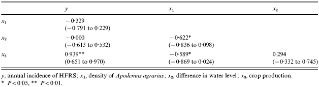
y, annual incidence of HFRS; x1, density of Apodemus agrarius; x2, difference in water level; x3, crop production.
P<0·05, ** P<0·01.
Table 2.
Partial correlation coefficients (95% confidence interval) between variables controlling for x3
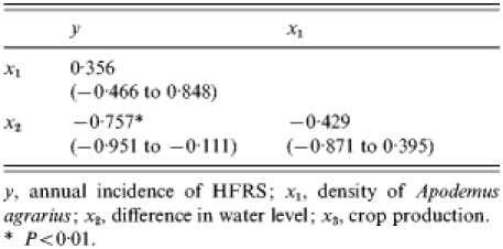
y, annual incidence of HFRS; x1, density of Apodemus agrarius; x2, difference in water level; x3, crop production.
P<0·01.
Autocorrelations
The autocorrelations, by a lag of year 1, 2, …, 10, were respectively 0·60, 0·09, −0·39, −0·49, −0·46, −0·18, 0·00, 0·18, 0·13, and 0·06 for annual HFRS counts (Fig. 2). The high positive correlations at a lag of year 1 and the high negative correlations at lags of years 4 and 5 reflect the strong quadratic form of the response. Similar patterns were also observed from the plots of the partial autocorrelations.
Fig. 2.

Autocorrelation coefficients of HFRS.
Model building
The results of the linear autoregression time-series model (model I) showed that the log incidence rates of HFRS was statistically significantly associated with crop production (P<0·01), and was marginally positively associated with the density of A. agrarius (P=0·09) and negatively (but not statistically significantly) associated with difference in water level (P=0·14). No significant lag effect was found in this model and the analysis of variance (ANOVA) shows that the model provided a reasonable fit to the data (F=61·87, P<0·01). The R2 was 98% (Table 3).
Table 3.
Regression coefficients of three models
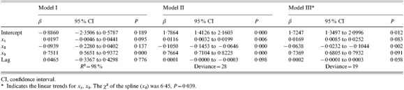
CI, confidence interval.
Indicates the linear trends for x1, x2. The χ2 of the spline (x2) was 6·45, P=0·039.
The parameter estimates of the Poisson autoregression model (model II) indicate that there were statistically significant associations between annual counts of HFRS and three predictors after adjustment for the size of the population (Table 3). It appears that the HFRS counts were positively associated with density of A. agrarius and crop production, but were inversely associated with difference in water level (P<0·01). No significant lag effect was found in this model. The deviance of residuals was 28 (Fig. 3).
Fig. 3.

Autocorrelation of residuals in three models. The dotted lines indicate the upper and lower levels of 95% confidence intervals; □, autocorrelation function coefficients.
The analysis of the Poisson autoregression GAM using Poisson link (model III) shows that adding a spline smoother (see Appendix) to both density of A. agrarius and difference in water level reduced the residual deviance from 28 to 19 (Table 3).
Goodness of fit
Shapiro–Wilk tests appear to meet the assumption that the standardized residuals were normally distributed (P>0·05). There was no significant autocorrelation between residuals in any of the three models in the Box–Ljung test (P>0·05) (Fig. 3). The validation analyses indicate that the model III had high accuracy over the predictive period (model I: r.m.s. error 16·09; model II: r.m.s. error 5·45; model III: r.m.s. error 3·97).
Estimation and prediction
Figure 4 depicts the adequacy of estimation through the closeness of the fitted and observed values for years 1984–1994. It also provides a comparison of the predictive ability of the models for 1995. Model III appeared to be the best for both estimation and prediction (predicted value for 1995: model I, 274; model II, 255; model III, 241; actual value, 218).
Fig. 4.

Model fitting and calibration with the time-series data of HFRS.
Model comparison
The three regression models appeared to have similar outputs. In general, the HFRS incidence was positively associated with density of A. agrarius and crop production and inversely associated with the water level in Huai River. However, the Poisson autoregression spline model (i.e. model III) appeared to have the best goodness-of-fit and short-term predictive ability (Table 3, Fig. 4).
Discussion
Using different modelling approaches, we confirmed our previous findings that the transmission of HFRS was associated with climatic and occupational factors [3, 13]. We also found that a Poisson GAM time-series spline model appeared to be the most suitable in the assessment of the relationship between the transmission of HFRS and the three independent variables, although a log-transformed linear regression model with normal errors and a Poisson GLM also seemed to perform reasonably well.
Logarithmically transformed linear regression models have been commonly used in the assessment of determinants of ‘high’ frequency rates [19, 20]. In the development of a linear regression model, the most common approach for modelling is through least squares, due to its computational tractability, its minimal (but strong) assumptions for hypothesis testing and its applicability for a wide class of problems [4]. This applicability is enhanced when the problem allows for transformations of the data, as in the development of model I. The traditional method of dealing with typically skewed data is to apply a transformation, such as the log transformation of the dependent values, in order to improve both symmetry and homogeneity of variance in the residuals. However, there is a fundamental flaw with this approach: If the original relationship is linear, it is no longer linear after the transformation. If we fit a straight line and then transform back to the original scale, the fit is no longer linear. Moreover, independence between the mean and variance is not always satisfactorily achieved in the transformation.
There is a difference between the Poisson regression and log-transformed linear model. The former entails the assumption of a Poisson likelihood whereas the latter assumes a normal distribution for the residuals. Poisson regression models have gained popularity for the analysis of time-series data in medical and public health research, because many biological phenomena are well described by Poisson distribution [19].
GLM extended normal regression models to accommodate both non-normal response distributions and transformations to linearity [21]. Furthermore, GAM extended the GLM by fitting non-parametric functions to estimate the relation between the response and the predictors [22]. GAMs assume that the mean of the dependent variable depends on an additive predictor through a nonlinear link function (as opposed to a linear link function under a GLM). Both GAMs and GLMs permit the response probability distribution to be any member of the exponential family of distributions [17].
In this study, we found that the transmission of HFRS incidence was positively associated with the density of A. agrarius and crop production, but was inversely associated with difference in water level. Although model I performed reasonably well, models II and III provide a much more straightforward interpretation of the influence of the explanatory variables (especially difference in water levels) on HFRS incidence. Under model I, difference in water level was not statistically significant, but became statistically significant after controlling for crop production. Although this was not unexpected in light of the high correlations between the three explanatory variables, the resultant inferences about the role of these three variables in estimating and predicting HFRS incidence become more complicated. Under model II and more obviously under model III, this difficulty disappears because the increased flexibility of the model allows a clearer expression of the contribution of each variable. Model III may be more appropriate as demonstrated by goodness-of-fit and model diagnosis outcomes. Importantly, under model III all variables were statistically significant at the 5% level and the predicted HFRS incidence was demonstrably closer to the observed incidence for the year 1995.
This study may have three major implications. First, our data demonstrate that climatic and occupational variables are key determinants of HFRS transmission, particularly in low-lying areas. These results were confirmed by different modelling approaches, and therefore, should be incorporated in the public health risk-management planning for HFRS. Second, the findings of this study may assist local public health authorities to utilize the model developed in this study to identify the communities that require particular attention, and to mobilize limited resources to effectively control and prevent outbreaks of HFRS during epidemic seasons. Finally, this modelling approach may also be applicable to a wider scientific community, particular those who are interested in the assessment of risk factors of disease transmission.
Some limitations of this study should be acknowledged. First, our analyses were confined to a small number of covariates, measured at a relatively large timescale (i.e. annually). A more refined analysis could use more frequent time-dependent covariates (e.g. weekly and monthly) to incorporate information on changes that occurred over the different time intervals at the expense of smaller (possibly zero) responses per unit of time. Second, the occurrence of HFRS is complex. Many factors could affect the incidence of HFRS, such as disease control programmes, the virus carrier rate among rodents, population movement and nutritional status. It may add some value to include other explanatory variables in the model. Third, explanatory variables may interact with each other in the occurrence of HFRS. For example, regular periods of low rainfall may benefit crops and vectors, while other crops may also promote the population of A. agrarius. Both of these factors may, therefore, contribute to the increased incidence of HFRS. However, high rainfall may have an opposite effect, especially in low-lying areas. The interactive effects of explanatory variables were not assessed due to the limited availability of the data. Finally, the study only focused on a low-lying area in Anhui, China. The results must be interpreted with caution as the situation in other areas may differ substantially.
In conclusion, similar results were obtained by using different modelling approaches. However, a GAM model appears to be the best fit with the time-series data in this study, and it may also have wider applications in the research of disease transmission.
Appendix
Least-squares linear, time-series model (model I)
The standard linear regression time-series model assumes the expected value of Y has a linear form
the constant term is denoted by β0, the autoregressive coefficient by φ and the regression coefficient by β. Estimation is typically by least-squares or maximum-likelihood methods.
GLM with a Poisson link time-series model (model II)
GLMs extend linear models by allowing for a link between f(X) and the expected value of Y. GLM is composed of a likelihood [here Y∼Poisson (μ)] which is a member of the exponential family by a linear function of the explanatory variables (Ŷ(t)=φY(t−1)+β0+β1X1+ … +βpXp) and a link between these two components [log(μ)=f(x)]. Estimation is typically calculated by maximum-likelihood methods.
GAM with Poisson link time-series spline model (model III)
GAMs extend the GLM by allowing for (smooth) nonlinear functions in f(X), so that Ŷ(t)=φY(t−1)+s0+s1(X1)+⋅⋅⋅+sp(Xp), where s0(.), …, sp(.) are smooth functions. These functions are estimated in a non-parametric fashion. In model III cubic splines are used to define si(X), i=1, …, p.
DECLARATION OF INTEREST
None.
REFERENCES
- Wu X, Lian Z. Epidemiology. 3rd edn. Beijing: People’s Medical Publishing House; 1996. Epidemic haemorrhagic fever; pp. 244–256. , pp. [Google Scholar]
- Wu G. Progress in the epidemiologic study of hemorrhagic fever with renal syndrome in China in recent years. Zhonghua Liu Xing Bing Xue Za Zhi. 2003;23:413–415. [PubMed] [Google Scholar]
- Bi P et al. Seasonal rainfall variability, the incidence of haemorrhagic fever with renal syndrome, and prediction of the disease in low-lying areas of China. American Journal of Epidemiology. 1998;148:276–281. doi: 10.1093/oxfordjournals.aje.a009636. [DOI] [PubMed] [Google Scholar]
- Fabien V et al. Use of the generalised linear model with Poisson distribution to compare caries indices. Community Dental Health. 1999;16:93–96. [PubMed] [Google Scholar]
- Sheppard L et al. Effects of ambient air pollution on nonelderly asthma hospital admissions in Seattle, Washington. Epidemiology. 1999;10:23–30. [PubMed] [Google Scholar]
- Braga A, Zanobetti A, Schwartz J. The effect of weather on respiratory and cardiovascular deaths in 12 U.S. cities. Environmental Health Perspectives. 2002;110:859–863. doi: 10.1289/ehp.02110859. [DOI] [PMC free article] [PubMed] [Google Scholar]
- Gouveia N, Fletcher T. Time series analysis of air pollution and mortality: effects by cause, age and socioeconomic status. Journal of Epidemiology and Community Health. 2000;54:459–472. doi: 10.1136/jech.54.10.750. [DOI] [PMC free article] [PubMed] [Google Scholar]
- Tobias A et al. Use of Poisson regression and Box–Jenkins models to evaluate the short-term effects of environmental noise levels on daily emergency admissions in Madrid, Spain. European Journal of Epidemiology. 2001;17:765–771. doi: 10.1023/a:1015663013620. [DOI] [PubMed] [Google Scholar]
- Tong S, Hu W. Different responses of Ross River virus to climate variability between coastline and inland cities in Queensland, Australia. Occupational and Environmental Medicine. 2002;59:739–744. doi: 10.1136/oem.59.11.739. [DOI] [PMC free article] [PubMed] [Google Scholar]
- Dominici F et al. On the use of generalized additive models in time-series studies of air pollution and health. American Journal of Epidemiology. 2002;156:193–203. doi: 10.1093/aje/kwf062. [DOI] [PubMed] [Google Scholar]
- Hastie T, Tibshirani R. Generalized Additive Models. New York: Chapman & Hall; 1990. [Google Scholar]
- Tabachnick B, Fidell L. Using Multivariate Statistics. New York: Harper Collins College Publishers; 1996. [Google Scholar]
- Bi P et al. Climatic, reservoir and occupational variables and the transmission of haemorrhagic fever with renal syndrome in China. International Journal of Epidemiology. 2002;31:189–193. doi: 10.1093/ije/31.1.189. [DOI] [PubMed] [Google Scholar]
- SAS Institute Inc. SAS Procedure Guide, Version 8. Cary, NC: SAS Institute Inc.; 1999. [Google Scholar]
- Box G, Jenkins G. Time-series Analysis: forecasting and control. San Francisco, CA: Holden-Day; 1970. [Google Scholar]
- Makridakes S, Wheelwright S, Hyndman R. Forecasting: methods and applications. New York: John Wiley & Sons Inc.; 1998. [Google Scholar]
- Venables W, Ripley B. Modern Applied Statistics with S-PLUS. New York: 1999. : Springer, [Google Scholar]
- SAS. The SAS System for Windows, Version 9.1. Cary, NC: SAS Institute; 2005. [Google Scholar]
- Mark W. Epidemiology: study design and data analysis. London: Chapman & Hall; 1999. [Google Scholar]
- Clayton D, Hills M. Statistical Models in Epidemiology. Oxford, UK: Oxford University Press; 1994. [Google Scholar]
- McCullagh P, Nelder J. Generalised Linear Models. London: Chapman & Hall; 1989. [Google Scholar]
- Green P, Silverman B. Nonparametric Regression and Generalized Linear Model. London: Chapman & Hall; 1994. [Google Scholar]