Design and analysis of small-scale transmission experiments with animals

SUMMARY

Interactions between pathogens and hosts at the population level should be considered when studying the effectiveness of control measures for infectious diseases. The advantage of doing transmission experiments compared to field studies is that they offer a controlled environment in which the effect of a single factor can be investigated, while variation due to other factors is minimized. This paper gives an overview of the biological and mathematical aspects, bottlenecks and solutions of developing and executing transmission experiments with animals. Different methods of analysis and different experimental designs are discussed. Final size methods are often used for analysing transmission data, but have never been published in a refereed journal; therefore, they will be described in detail in this paper. We hope that this information is helpful for scientists who are considering performing transmission experiments.

INTRODUCTION

Prevention and control of infectious diseases in animal husbandry are important topics in veterinary research. Most of this research is focused on the reduction of the clinical signs (i.e. disease). However, an important characteristic of an infectious disease is that the causative agent spreads from one animal to another, and part of the processes that may result in infection are determined by the interaction between individual animals within a population. Depending on the disease of interest, one might focus on the control of the spread of the infection in the population rather than controlling the disease in individual hosts. Reasons for such an approach are that (i) it is the most effective way to control disease, (ii) it is directly related to the trade restriction associated with not being free from disease, (iii) it might prevent disease in other host species (in particular humans). The combination of the interaction between the infectious agent and the individual host, and the interaction between hosts determines the course of the infection in a population. Therefore, these interactions at the population level should also be considered when studying the effectiveness of control measures for infectious diseases.

When measuring the effect of control measures on the spread of pathogens in a population, there are two crucial questions to be answered: (1) to what extent does an infection spread, and (2) is the observed effect of a control measure significant and relevant? Therefore, transmission of the pathogens has to be quantified. A useful variable for quantification is the reproduction ratio, R. The basic reproduction ratio, R₀ is the average number of secondary cases caused by one typical infectious individual in a completely susceptible population during its entire infectious period [1]. Since the use of R₀ is restricted to the situation without intervention, the reproduction ratio is usually described by R in situations with control measures. R has a threshold value equal 1. This implies that an infection may spread when R>1, possibly resulting in a major outbreak, and will fade out when R<1, possibly resulting in a minor outbreak [1]. Thus, control measures will be most effective when they can bring R to a value below 1.

Transmission can be quantified in laboratory experiments and field studies. The main advantage of a laboratory experiment is that it offers a controlled environment in which the effect of a single factor can be investigated, while variation due to other factors is minimized. Furthermore, experiments can be less expensive and less time-consuming than field studies. Consequently, more treatments or control scenarios can be evaluated, even those that are not yet actually used or those that cannot be studied under field conditions (e.g. exotic diseases). A disadvantage of experiments is, however, that extrapolation of the results may be difficult.

The first quantitative transmission experiments were published by Greenwood et al. [2], who studied transmission of a bacterium between mice, and were further analysed by Kermack & McKendrick [3, 4], Anderson & May [5] and De Jong et al. [6]. More experiments that were carried out brought very useful data on the characteristics of infections and/or to the effectiveness of control measures. From these experiments, knowledge on the design and analysis of transmission experiments has been gained, as well as insight into transmission characteristics and interpretation of data of several infectious diseases.

Since the insights gained by these experiments, have been described in various papers, the aim of our paper is to give an overview of these insights, which can be helpful for other researchers who are considering performing transmission experiments. We focus on small-scale animal experiments, and on diseases caused by viruses and bacteria. First, we will give a brief description of a transmission experiment, and we will discuss biological aspects of an experiment: the infection model, and the diagnostic possibilities to monitor the infection chain. Second, we will discuss the analysis of the data with various methods and models. Third, we will discuss the interpretation of the observations and the mathematical and statistical results.

BIOLOGICAL ASPECTS OF TRANSMISSION EXPERIMENTS

Basically, an infection is started in a group of animals, housed together in an isolated unit, by inoculation of some animals in the group and contact exposure of the other animals to the inoculated [7]. The infection chain is monitored by taking samples from individual animals to diagnose a possible infection chain. The number of contact infections, either at the end of the infection chain or during the course of the infection in the group (i.e. a local epidemic), are used for statistical analysis to quantify transmission or to test the effect of a control measure. Mathematical models are used as the basis of the statistical methods to analyse and interpret the results.

The above description seems straightforward, but when intending to perform a transmission experiment, each single aspect has to be considered very carefully. In the following sections, different aspects, bottlenecks and solutions for developing and executing a transmission experiment will be described.

Starting the infection chain

An infection has to be started artificially, which implies that a suitable method to get infectious animals is needed. In many mathematical models used for the analysis, ‘equal infectiousness’† for all infected animals is assumed, independent of how they became infected. Such an assumption would allow extrapolation to more generations of infection (cascade of new infections), which may not be observed experimentally, but which may occur in field populations.

The infection chain is often started by direct inoculation of one or more animals with a certain dose, route and infection moment. The assumption of equal infectiousness will be put under pressure, when inoculated animals differ in infectiousness from contact-infected animals (illustrated by Fig. 1). For example, in an experiment with pseudorabies (PRV) in maternally immune pigs, the inoculated piglets shed measurable amounts of virus, whereas in the contact-infected piglets (detected by seroconversion) no virus excretion was observed [8]. Then, transmission may be overestimated and other ways to obtain infected animals have to be developed. Another example of differences in infectiousness can be found in vaccination experiments with classical swine fever (CSF) [9] and foot-and-mouth disease (FMD) [10]. Artificially inoculated vaccinated animals did not become infectious in the vaccinated groups whereas they did become infected in the unvaccinated groups. In these situations, a transmission experiment might not be necessary, given that we are confident that inoculation reflects exposure in the field. If not, the extended transmission experiment which is described in the next paragraph may be used.

Fig. 1.

Evaluation of a transmission experiment with a treatment and control group. If the experiment only consists of a control group (i.e. to estimate transmission parameters) the tree will not include the subtree about the treatment group.

When artificial inoculation results in a presumed higher infectiousness of inoculated animals than contact-infected animals, the design of a so-called extended experiment might be more suitable (see e.g. refs [8, 11]). In this experiment, artificially inoculated animals are used to infect contact animals to create infectious animals. These infectious animals are subsequently placed with susceptible animals to start the infection chain in the actual experiment. The main advantage of this design is that the first generation of contact-infected animals more closely resembles a natural infection even when the initial inoculation is artificial (e.g. by injection). A disadvantage is, however, that the initial infection process is less controlled and that the timing of the moment at which the infectious animals should be placed with the susceptible animals is hard to determine.

Monitoring the infection chain

The type of information needed for quantification of transmission depends on the infectious agent, the diagnostic tools, and the subsequent mathematical analysis. It is important to consider which observations can be made and how these observations relate to the infection states assumed in the model used in the statistical analysis. When estimating transmission, it is assumed that all infected animals are equally infectious (samples from the same distribution of infectiousness), and all contact-exposed animals are equally susceptible.

In the mathematical model, an individual is assumed to be infected when the individual is infectious to others. Note that not all infected animals need to be infectious, nor does an infected state automatically mean that the animal will become diseased, or, vice versa, that more diseased animals are also more infectious. Diagnostic tools should ideally be able to determine whether an animal has been infected in such a way that it also is infectious to others. Moreover, since the infectivity and length of the infectious period varies between different infectious diseases, the frequency of sampling should be considered, as well as the duration of the experiment to allow the occurrence of contact infections.

Several diagnostic tools are available to detect the presence of the agent or a former contact with the agent, e.g. clinical examination, antigen detection tests, and immunological assays. Clinical examination can be relevant, but is often not very precise in determining the moment of infection, nor is it a measure for infectiousness, since virulence and infectiousness are not necessarily correlated (e.g. PRV [12]).

Antigen detection seems a more appropriate way of detecting an infection. Various techniques are available to detect infectious agents, e.g. virus isolation, culture of bacteria, antigen tests and PCR. The question remains how antigen detection is correlated with the infectious state. Difficulty may arise when the agent is isolated from a site where it will not be shed (e.g. determination of viraemia), when it is shed intermittently, or when the diagnostic technique does not distinguish between live and inactive particles (e.g. PCR). Moreover, the link between amount of infectious agent isolation and infectivity to other animals is not always clear. For Actinobacillus pleuropneumoniae (App) infections in pigs, for example, it was concluded that the number of bacteria isolated from the nasal swab was closely related to infectivity, and the number of bacteria isolated from the tonsillar swabs not, although more frequently higher numbers of bacteria were isolated from tonsillar swabs than from nasal swabs [11].

Immune responses are often used as an indirect way of detecting infections, e.g. serology, tuberculin tests or lymphocyte proliferation assays. These tools can be used when the experiment lasts long enough for animals to develop an immune response after exposure. However, these tools also have disadvantages. First, infected animals may not always develop an antibody response upon infection, as shown for pigs vaccinated with the marker vaccines E2 against CSF [13], and for App infections in pigs [14]. Second, in vaccination experiments it might be impossible to distinguish between immune responses triggered by vaccination and by actual infections. Third, immunological assays are expected to be even less informative about whether animals were also infectious than are antigen detection assays. When an animal becomes seropositive but ‘not infectious’, one could assume this animal to be a ‘dead end host’, thus, not infected at all (e.g. ref. [8]). Then, transmission might be overestimated if this animal is categorized as a case. Fourth, the moment of infection is difficult to estimate from an immune response, because, in general, this runs far behind the moment of infection. Although this does not change the interpretation of the final size of an outbreak, it hampers the estimation of the infection rate parameter β.

In conclusion, although several diagnostic tools are available to detect the presence of an infectious agent in an animal or to detect a previous exposure to an infectious agent, the link between the measurements in individual animals with transmission in a population is not always straightforward. Transmission might be over- or underestimated when using a certain diagnostic tool. Moreover, the transmission experiments themselves may be used to determine the relation between measurements in individual hosts and the infectivity. For example in Bouma et al. [8], maternally immune piglets became infected with PRV after contact exposure to inoculated maternally immune piglets, as measured by seroconversion. However, these allegedly infected piglets failed to cause seroconversion in a second generation of maternally immune contact piglets. Thus, some measure is suggested to be the measure for infected and hence infectious individuals, then animals labelled infected by that definition are housed with contact animals and it is measured whether they, in turn, by the same definition get infected.

The interpretation of the results, whether animals are infected or infectious and how the experiments can be analysed will be discussed in the following sections.

MATHEMATICAL ASPECTS OF TRANSMISSION EXPERIMENTS

Stochastic susceptible–infectious–removed (SIR) model

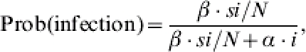
Mathematical models are necessary to analyse nonlinear processes of directly transmitted infections. A suitable basic model (i.e. as simple as possible but with sufficient complexity to make a sound statistical analysis) is the stochastic SIR model [15, 16]. This model describes how two events can occur with an individual: the individual can become infected and can recover from the infection. Infection occurs when an infectious individual transmits the infection to a susceptible individual. In the model it is assumed that the contact rate γ of each individual with other individuals is constant and the probability p that transmission takes place given a contact is also a constant. From that it follows that the rate at which one susceptible individual would become infected equals β (=γ⋅p) in a population with only infectious individuals. In a population with infectious and susceptible individuals this rate would be β(I/N) where I is the number of infectious individuals and N the total number of individuals present. Thus at the population level the rate at which susceptible individuals become infected is β⋅S⋅(I/N) where S is the number of susceptible individuals. Recovery is when the infectious individual ceases to be infectious. It is assumed that recovery occurs at a constant rate independent of the infection and exposure history of that individual. The duration of the infectious period is a stochastic variable that has an exponential distribution with an expected duration equal to 1/α. At the population level recoveries occur with rate αI. In summary the stochastic SIR model can be given by the following expressions:

From which it follows that the average number of new infections caused by one infectious individual in a totally susceptible population (R) equals β/α.

The SIR model, and thus also the statistical methods based on the SIR model, are based on a number of assumptions. Some of them have already been mentioned. In summary, the most important assumptions are: all animals within the population have random contacts with each other; every class S, I and R consists of a homogeneous group of individuals; the infection rate is constant during the entire infectious period; the duration of the infectious period is exponentially distributed; and each recovered animal is fully immune to subsequent infection. Therefore, application of statistical methods based on the SIR model requires these assumptions to be checked carefully.

Statistical methods to quantify transmission

The choice of the statistical method depends on the type of infection (host–agent relationship) and the type of data collected in the experiment. We distinguish two groups of statistical methods useful for analysis of transmission experiments. In one group the input is the total number of animals infected at the end of the experiment (in relation to the number of susceptible and infectious animals at the start of the experiment). In the other group of methods the number of new infections during the experiment is the input (in relation to the number of susceptible and infectious individuals in the course of the experiment). Methods based on the final size (FS) algorithm, the martingale estimator and methods based on the transient state (TS) algorithm fit into the first group, whereas the MaxDiff method and the GLM method fit into the second group. Table 1 gives an overview of the characteristics of the different statistical quantification methods. We will discuss the methods in the next sections and will describe the methods based on the FS algorithm in detail. Most methods are described in detail elsewhere; therefore we will not describe them here. The FS methods were first described by De Jong & Kimman [7]. However, a more extensive description is only given in a proceeding paper [17] that is not available to all scientists. For that reason this method is described in detail here.

Table 1.

Overview of the characteristics of different methods to quantify transmission (source: [22])

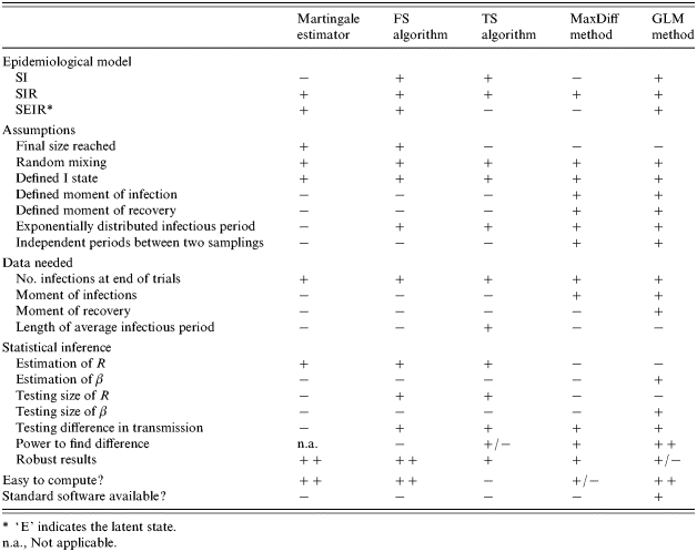
^*‘E’ indicates the latent state.

n.a., Not applicable.

FS methods

The stochastic SIR model can be simplified when only the final outcome is studied, i.e. the number of infectious or susceptible individuals at the end of the experiment [7]. The final outcome can only be studied for infections where individuals recover and where the experimental period is long enough so that either all infected individuals do recover or all susceptibles are infected before the end of the experiment. The final outcome is also called the ‘final size’ of the experiment. The variable to be studied can either be the number of new contact infections or the the number of animals that escaped infection until the end of the experiment.

Statistical analyses to test hypotheses on R or to estimate R are based on a known distribution over all the possible FS outcomes, i.e. the FS distribution. The FS distribution is described by a set of functions that only depends on R. These functions can be deducted from the stochastic SIR model by ignoring the timing of infection and recovery events, which is described below.

The population of individuals that we observed is classified in three mutually exclusive categories: susceptible (S), infectious (I), and recovered (R). Therefore, the population can be represented by the pair (s, i), i.e. the number of susceptible and infectious individuals. The probability p(s, i) is the probability that the population state is (s, i) at any moment in time, i.e. from the start of the experiment until infinity. These probabilities depend on the parameter R and the number of susceptible and infectious individuals at the start of the experiment (s₀, i₀).

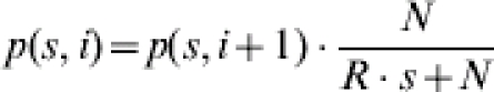
Given that the population state is (s, i), it will be (s – 1, i+1) if a susceptible individual becomes infected or it will be (s, i – 1) if an infectious individual recovers. Thus, either an infection event occurs with probability:

(1)

or either a recovery event occurs with the complementary probability

Since the reproduction ratio is R=β/α, the probability of an infection event can be simplified:

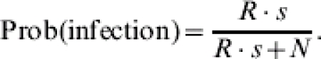(2)

The simplification clearly illustrates that the FS distribution only depends on R and not on β and α separately.

The probability of having reached an arbitrary state (s, i) in the infection chain during the whole epidemic process can be calculated based on the infection and recovery probabilities:

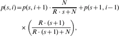(3 a)

for 0⩽s+i⩽s₀+i₀, 0⩽s⩽s₀, and 2⩽i and

(3 b)

for i=0, 1. Since the start situation of a trial is known, i.e. p(s₀, i₀)=1, the probability for each other state in the infection chain can be calculated.

The FS probability distribution is given by the set of the probabilities of all possible FS situations, i.e. p(s, 0) for 0⩽s⩽s₀. From the definition of p(s, i) and the fact the FS states are absorbed it follows that: 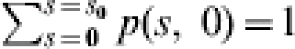. For example, given that the infection chain starts in state (5, 5), it will end in one of the following absorbing states: (0, 0), (1, 0), (2, 0), (3, 0), (4, 0) or (5, 0). Thus, the FS probability distribution consists of the corresponding six state probabilities. With the probability distribution of all trials within one experiment, a joint probability distribution of the whole experiment can be calculated easily. Subsequently, different tests on the value of R can be performed and an estimate on R can be obtained.

In the test and estimation methods presented below equal numbers and sizes of transmission trials are assumed for simplicity of notation. However generalization to unequal numbers of trials or even unequal numbers of individuals per trial is possible and straightforward.

Obtaining a point estimate for R

Given a value of R, the probability of each possible outcome (final size) can be calculated exactly from the FS probability distribution. Conversely, given the outcome of a transmission experiment, R can be estimated using the maximal likelihood estimation as follows. Suppose m transmission trials have been performed each with (s₀, i₀) as initial state. Let X be the number of contact infections in the jth trial. Then, the probability distribution of outcomes X₁, …, X_m in m trials is:

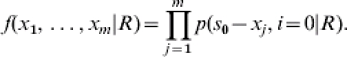(4)

When changing our point of view, we alternatively denote the corresponding likelihood function f(R|x₁, …, x_m), where s₀−x_j denotes the number of susceptible individuals in trial j escaping infection. The value of R that maximizes the likelihood function is called the maximum likelihood estimate of R.

Testing against threshold value 1

One-sided and two-sided statistical tests on R can be based on probability distributions like those given in equation (4). For eradication of an infectious agent, R should be brought below 1. To show that R<1 the composite null hypothesis H₀: R⩾1 should be considered. This hypothesis can be tested by calculating the probability that k or less contact infections occur in m trials under the condition R=1:

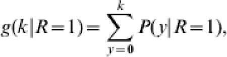(5)

which leads to the highest p value (thus a conservative test). p(y) is the multiplication of all distributions [eqn (4)] where 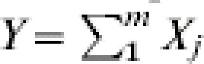. The critical region of the test, i.e. where H₀ is rejected is formed by all values of y below k where k is the maximum value for which g(k|R=1)=0·05 still holds.

Another hypothesis that may be of interest is H₀: R⩽1. Rejecting this hypothesis implicates that R might well be >1, making it uncertain whether the infectious agent can be eradicated from the population and meaning that major outbreaks can occur. To reject H₀: R⩽1 the probability that the observed number of contact infections y or more contact infections would occur in m trials under the null hypothesis should be smaller than 0·05.

Obtaining a confidence interval for R

A two-sided 95% confidence interval (95% CI) for R is constructed by finding all R such that H₀: R=r is not rejected in a test with error level of 0·05. A natural choice for a test statistic is Y, as before, the total number of contact infections in m trials. Then, given Y=y the 95% CI is constructed by collecting all R values such that the hypothesis H₀: R=r would not be rejected. In case of extreme outcomes, where none or all susceptible individuals were contact-infected, a one-sided confidence interval would be more appropriate.

Testing the difference in R between two treatment groups

One reason to perform a transmission experiment is to determine the effect of an intervention on the transmission of an infectious agent. We can compare the levels of transmission under two different experimental conditions or treatments, e.g. vaccinated or not vaccinated. In the null hypothesis there is no difference in transmission between the two treatment groups, H₀: R_con=R_treat, whereas the alternative hypothesis is that the intervention has reduced the transmission, H₀: R_con>R_treat. (Here R_con denotes the R in the control group, and R_treat the R in the treatment group.) Because we assume that the treatment will not result in an increased R, a one-sided test is discussed, but modification to a two-sided test is straightforward.

A natural test statistic for this test is the total number of contact infections observed in the control trials (Y_con) minus the total number of contact infections in the treatment trials (Y_treat):

(6)

To test H₀: R_con=R_treat, the probability that the difference in the number of contact infections is larger than or equal to the observed difference in the number of contact infections z, has to be calculated under the condition R_con=R_treat. The probability of observing difference z is the sum of all possible products of the two probability functions – five for each treatment group:

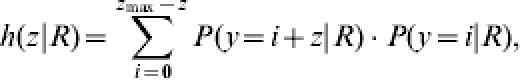(7)

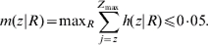
where z_max is the maximum difference possible. H₀ is rejected if the probability of having the observed difference z or more is <0·05 for any value of R, i.e. if

(8)

The reason that the maximum probability m(z|R) is <0·05 for any arbitrary R chosen is because H₀: R_con=R_treat is a composite null hypothesis. The R for which that is obtained is possibly different for each observed outcome.

Transient state (TS) methods

TS methods are based on an algorithm that generates a time-dependent probability distribution over all (transient and absorbing) states of the infection chain. The TS algorithm takes the time course of the experimental epidemic or infection chain into account. The TS algorithm is described in detail by Velthuis et al. [18].

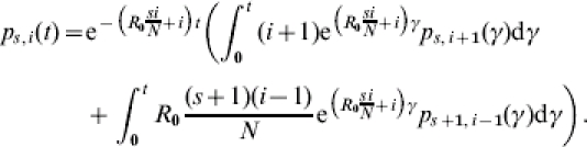
In summary, the adjacent state probabilities that can occur given the start condition of the experiment satisfy the forward differential-difference equations:

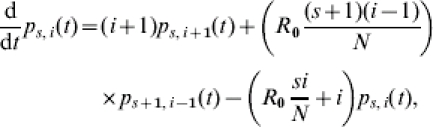(9)

for 0⩽s+i⩽s₀+i₀, 0⩽s⩽s₀, and 0⩽i⩽s₀+i₀. Subject to the initial value 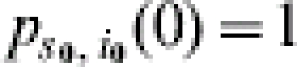, this equation can be solved using standard methods. The solution that we call the TS algorithm can be used to calculate a continuous-time state probability for each state in the epidemic process:

(10)

The practical use of the TS algorithm is restricted to experiments with only few individuals. This is because its high degree of recursiveness may cause numerical problems, memory limitation or long computation time [15, 19, 20]. The high degree of recursiveness in the TS algorithm disappears if time tends to infinity, turning the TS algorithm into the readily applicable FS algorithm, which is described in the section about FS methods.

The estimation methods and testing methods based on the TS probability distribution are similar to the methods that are described for the FS probability distribution. The input needed for these methods is the number of contact infections at the end of each trial and the average infectious period. The latter is often unknown.

When planning to use a quantification method based on the TS algorithm, a FS situation does not necessarily need to have been reached, but the duration of the experiment in terms of the average infectious period has to be known. This information, however, is often not available. A solution for this problem is to assume a worst-case scenario, e.g. the average infectious period equals the expected lifespan of the animals, which is very well defined for farm animals. Assuming this, it is possible to express the duration of the transmission experiment in terms of the average infectious period and to use the TS algorithm.

Martingale estimator

By applying a method of moments for martingales as described in Becker ([21], chapter 7) an estimate of R, the martingale estimate, can be obtained as described in Bouma [12]. The martingale estimate converges to a true value if more data become available, not only for the stochastic SIR model as assumed here, but also for other more general models.

The FS and TS methods are based on the assumption that the infectious period is exponentially distributed, whereas the martingale estimator is not. Furthermore, the martingale estimator is based on large populations only, while the FS and TS methods are not limited to population size. Thus, it is questionable whether the use of the martingale estimator for experiments with small groups of animals is valid. However, if all susceptible animals become contact-infected in all transmission trials the martingale estimator might be a useful method to estimate R, since the estimate of R will go to infinity when using the FS or TS maximum-likelihood estimate, while it converges to a true value when using the martingale estimator. This is because the martingale estimator uses the remaining length of the individual infectious periods immediately after the last infection occurred as extra information.

MaxDiff method

The MaxDiff method is developed to detect a difference in transmission between two treatment groups that occurs during the experiment but is not visible at the end of the experiment, i.e. the difference in the number of contact infections grows during the experiment, but disappears at the end (Fig. 2). The MaxDiff method is described in detail by Velthuis et al. [22]. The test statistic used in the MaxDiff method is the maximum difference in the number of contact infections that have occurred during the course of the experiment (i.e. the so-called maximum difference). The probability distribution over all possible maximum differences under the null hypothesis (which is that there is no difference in transmission) can be generated by Monte-Carlo simulations. The simulations are based on the transmission processes assumed in the stochastic SIR model and can be done for all experimental designs (s₀, i₀). With the probability distribution it can be tested whether the observed maximal difference lies within the critical region or not. The power of the MaxDiff test is also calculated with help of simulations. It appears that the power of the MaxDiff test is often sufficient to detect a difference in transmission between two treatments, while the power of the tests based on the FS or TS algorithms is not sufficient (Table 2). Especially when both R_con and R_treat are above threshold one [22].

Fig. 2.

Theoretical results of a transmission experiment that is stopped (dashed vertical line) before a final size situation has been reached in all trials (left panel) and two possible end situations that could have been observed when the final-size situations have been reached (right panels).

Table 2.

Power calculations of the different tests to find a difference in transmission between two treatment groups applied on data of a five-to-five transmission experiment with two trials per treatment

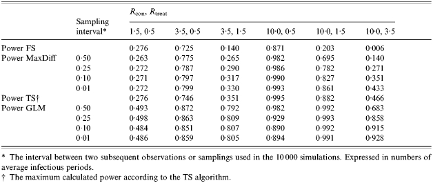
^*The interval between two subsequent observations or samplings used in the 10 000 simulations. Expressed in numbers of average infectious periods.

^†The maximum calculated power according to the TS algorithm.

Generalized linear models (GLM)

A different method to estimate a transmission parameter or to test hypothesis is based on a GLM. Becker [21] described the application of a GLM to epidemiological models in detail and used a specific version of the SIR model. An adapted version of a GLM to analyse transmission experiments is described by Velthuis et al. [14]. The GLM method is like all other methods also based on the stochastic SIR model. With the GLM method the infection rate parameter β can be estimated and the hypothesis about its size can be tested. The power to find a difference in transmission between two treatment groups is generally higher than all other methods that have been described above (Table 2).

A disadvantage of the GLM method is that it assumes periods between two subsequent samplings are independent of each other. This means that each susceptible animal at the start of a period has the same probability of becoming infected in the subsequent period. This is questionable, since the resistance of a susceptible animal to become infected may vary in time.

An advantage of the GLM method is that it can account for heterogeneous populations. One of the assumptions of the stochastic SIR model is that the classified groups in the different infection states (S, I or R) are homogeneous, i.e. all S animals are assumed to be equally susceptible, all I animals equally infectious per time period† and all R animals equally immune. The validity of this assumption can be questioned for particular applications, as illustrated, e.g. for the infectivity of App-infected pigs [11], or the difference in infectivity between PRV-inoculated pigs and contact-infected pigs [8]. Only with the GLM method it is feasible to include heterogeneity by adding variables that describe which fraction of an infection group meets a specific characteristic [14].

Another type of heterogeneity is observed in experiments where inoculated and contact animals are treated differently, e.g. when contact animals are vaccinated and inoculated animals not. In this situation only the effect of vaccination on the susceptibility can be tested with help of a GLM analysis [14].

Experimental design

Experiments are usually hampered by the limited number of animals that can be used. The design depends on the type of research question to be answered. The research question can be the estimation of a transmission parameter, or the question can be a comparison between transmission parameters due to different treatments. In the first two paragraphs of this section it is discussed which experimental design is optimal given the research question to be answered. In the third paragraph the duration of the experiment is discussed. In the fourth paragraph the choice of the statistical method will be discussed.

Number of trials and the number of susceptible and infectious animals at the start

The comparison of the different designs will be based on the power calculations with the FS method. This is because these power calculations are straightforward, while the calculations of other methods are not. The analysis is in practice often done with another method of analysis when this method gives higher power than the power obtained by the FS method. Thus, when we find a design that gives sufficient power with the FS method, it will certainly have sufficient power with the improved method. We compared different experimental designs based on equal numbers of animals. Two issues arise here, first, the ratio of inoculated animals vs. contact animals and second, the number of animals in each trial (and thus the number of replicates).

Ratio I₀/S₀

When designing an experiment, one can choose S₀ large and I₀ small, S₀ small and I₀ large or S₀ approximately equal to I₀. If the number of animals inoculated to become I₀ is small, there is a risk that these animals do not become infected and infectious. Moreover, if I₀ is chosen to be small and all inoculated animals become infected, minor outbreaks can occur due to chance processes, even if R>1. Figure 3 illustrates for two different experimental designs (I₀=1, S₀=9 and I₀=5, S₀=5) the FS distribution of the stochastic SIR model for R=5. The probability of having a minor outbreak is high (i.e. 0·18) when starting with one infectious individual, whereas this probability is zero when starting with five infectious individuals. If the number of susceptible animals is small it is possible that all susceptible animals can be infected, even if R<1. This suggests that a design with S₀≈I₀ is a good compromise.

Fig. 3.

The final-size distributions of the stochastic SIR model for R=5 for the experimental designs I₀=1, S₀=9 and I₀=5, S₀=5.

Number of animals and number of trial replications

Often the number of animals and isolation units available are limited. Therefore, a decision has to be made on how the number of animals will be distributed over the number of trials. First we will discuss the design when the goal is to estimate transmission parameters. We compared different designs by comparing the accuracy of estimated transmission parameters, i.e. the length of the confidence interval. To demonstrate the effect of experimental design on the estimated R value we simulated nine different experimental designs for three different values of R. The total number of animals in each design is 72 and the start condition of each trial is I₀=S₀. The designs differ only in the number of trials and the number of animals per trial, i.e. 36 trials×2 animals, 18×4, 12×6, 9×8, 6×12, 4×18, 3×24, 2×36 and 1×72. Per design we simulated 1000 experiments in two steps. First, the exact probability on each FS situation was calculated. With these probabilities the cumulative probabilities were calculated by adding up all probabilities from S=0 until any possible FS outcome. Second, we generated 1000 random values between zero and one representing random probabilities. The final size of a simulated experiment is X if the random probability is bigger or equal than the cumulative probability of x and lower than the cumulative probability of x+1. For each experiment the R value and its 95% confidence intervals were estimated under the FS assumption by the maximum-likelihood method. Per design, means of the 1000 estimates of R and the upper and lower boundaries of the 95% confidence interval are estimated (Fig. 4).

Fig. 4.

The 95% confidence interval of the estimated R value of 1000 simulated experiments of different sizes, given S₀ (total)=36; I₀ (total)=36; N₀ (total)=72; S₀≈I₀, in which R=0·5, 1·0 or 1·5, respectively.

From Figure 4 it can be seen that the confidence interval is smaller for designs with more animals per trial, although the difference for the different designs is small. Thus, one large trial is better than many small trials. However, it can be seen that there is not much difference between one large trial and a few repetitions of smaller trials. It is advisable to have at least some repetitions to make the conclusions more robust with respect to the model assumptions. Note that the maximum R value in Figure 4 is 1·5. It is not possible to estimate R with an acceptable accurate upper bound of the confidence interval for larger values of R. This is, however, not important for control strategies.

If transmission parameters of two populations are compared, the quantitative criterion in comparing designs is the power of the test, i.e. the probability of finding a difference if a difference is present. The power to find a difference in transmission between two treatment groups is calculated by adding the probabilities for all z in the critical region and then assuming the alternative hypothesis with separate values for R with and without treatment. Then the power is:

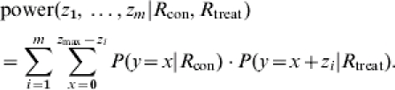(11)

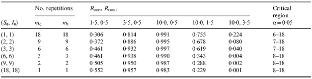
We compared different designs by comparing powers, given certain values of R_con and R_treat. The total number of animals in each design is again 72, the start condition of each trial is I₀=S₀ and the number of trials per treatment is equal (m_con=m_treat). The designs differ only in the number of trials per treatment and the number of animals per trial. Table 3 shows the different designs and their corresponding powers for different values of R_con and R_treat. The best design (in terms of the highest power) depends on the expected R_con and R_treat. If R_treat is expected to be <1 and R_con >1 the power is higher for designs with fewer trials and more animals per trial. However, the powers of all designs are sufficient (>0·8) if R_con is assumed to be 3·5 and 10·0, thus all designs are good enough to find a difference in transmission. However, if R_treat is expected to be >1 it is better to conduct an experiment with more repeated trials with fewer animals per trial. Especially if R_treat is close to but higher than 1 it is possible to find a difference in transmission by conducting one-to-one experiments.

Table 3.

Power calculations for different experimental designs to find a difference in transmission between two treatment groups

Duration of the experiment

The duration of an experiment should be long enough and the sampling scheme intensive enough to provide sufficient information about the infection chains for a sound analysis. The amount of information needed depends on the quantification method that will be used to analyse the data. For example, for a quantification method based on the FS algorithm, the local epidemics in the different trials should have reached a FS situation before the experiment ends. Therefore, ideally the experiment must last long enough to reach this final size. This is not feasible for all infections, since the timescale of the spread of an agent from one animal to another depends on the infection of interest and depends on the treatment that is evaluated (i.e. it is possible that an intervention slows down the transmission dynamics to such an extent that reaching a FS situation will take a considerable period of time).

When the final size is not reached at the moment at which the transmission experiment is terminated, important information might be missed. In Figure 2 two possible scenarios are presented. In the left panel of the figure the number of infections per treatment group in a transmission experiment is presented against time. The experiment was terminated at the moment where the FS situation had not been reached in all trials (dashed vertical line). If this experiment had lasted longer the results could have been different. For example, the difference in the number of contact infections could have increased (see the top right panel) or this difference could have decreased (see the bottom right panel). The different end situations would lead to different conclusions as to the significance of the difference in transmission between the two treatments.

The risk of drawing wrong conclusions if an FS-based method is used when the final size has not been reached in all trials has been investigated [18, 22]. From these studies it can be concluded that the R value is underestimated in these situation.

For analyses of a transmission experiment with a method based on the TS algorithm [22], the FS situation does not need to be reached in all trials. However, one of the inputs needed for this method is the duration of the experiment expressed as the number of average infectious periods, which is often unknown. A solution for this problem is to assume a worst-case scenario, namely, to assume that the average infectious period is equal to the expected lifespan of the animals, which is very well defined for most farm animal species. With this assumption the duration of the transmission experiment can be expressed in terms of the number of average infectious periods, and the methods based on the TS algorithm can be used to analyse the experiment.

For the use of the MaxDiff method the average infectious period does not need to be known [22]. When using the MaxDiff method to test for a difference in transmission between two treatment groups the experiment should last long enough to observe a significant difference in the number of contact infections (see Fig. 2). In this case, it should be possible to stop the experiment immediately when a significant difference in the number of contact infections has been reached. This would be good for animal welfare and, of course, cost reduction. However, note that if an experiment is stopped too early, extra information will be missed and the estimation of transmission parameters will be less precise.

Choice of method of analysis

Based on a chosen experimental design (i.e. a five-to-five experiment) the different methods of analysis will be compared in this section. One of the main considerations in choosing a test is the power of the test. In Table 2 the power to find a difference in transmission for a five-to-five transmission experiment with two trials per treatment group is calculated for different tests. The power of the MaxDiff test is generally less than the maximum power of the TS test, but will approach the maximum power if the sampling interval becomes extremely small. The power of the GLM test is large for almost all combinations of R_con, R_treat. The power of the MaxDiff test is only sufficiently large (>0·80) if R_con, R_treat is 10·0, 0·5 or if R_con, R_treat is 10·0, 1·5 with a sampling interval of 0·01. Slightly smaller powers (>0·70) are obtained for the combinations 3·5, 0·5 and 10·0, 1·5. The power increases with the difference between R_con and R_treat, but is insufficient in all but one scenario where R_con and R_treat are both >1. The sampling interval (in the range of 0·01–0·50 average infectious periods) has only a small influence on the power of the MaxDiff test when both R_con and R_treat are small, whereas it has more influence when R_con and R_treat are both >1. The largest effect is observed for the combinations 10·0, 1·5 and 10·0, 3·5, which can be explained by the on average small periods in which MaxDiff can be observed, 0·538 and 0·150 respectively.

Methods that used information of the course of the infection chain are more powerful than FS methods, especially when after treatment the R value is still >1. Thus, based on the power calculations the GLM and MaxDiff methods are always preferred for the analysis of the experimental data. However, these methods of analysis presuppose that measurements give sufficient information to know at which moments in time animals are susceptible, infected, infectious, and recovered. In reality such interpretation can only be given by making additional assumptions, for example about the duration of the latent period, about how infectious animals are based, for example, on excretion of the microorganism.

More information is not always available. In this case it is better to base your analysis on a method that needs less information. For example, the FS method can be used when the treatment reduces the R value to <1 and therefore the FS method has sufficient power to find a difference in treatment. If the FS situation is not reached in the experiment, one could choose to use the TS methods, although for these methods information about the duration of the infectious period is needed.

If one is only interested in the estimation of a transmission parameter and not in testing a difference in transmission between two treatments, the choice of a statistical method is different. With the FS and TS methods it is possible to estimate the R value based on the experimental data. With the GLM it is possible to estimate the two transmission parameters α and β separately. Having an estimate of both parameters it is also possible to estimate R.

Besides the power calculation, the choice of a statistical test depends also on other aspects, such as the quality of the available data, whether there is heterogeneity in the susceptible or infectious group of animals, whether a FS situation has been reached or not or whether the maximal difference in the number of infections between two treatments has already been reached or not. All these items have already been discussed in the previous sections. The decision tree given in Figure 5 illustrates a summary of all aspects that influence the choice of which method of analysis to use in which situation.

Fig. 5.

Decision tree illustrating which method analysis to use.

INTErPRETATION OF RESULTS

The results of the transmission that are based on experiments, in which a lot of factors have been controlled, may differ from the field situation and extrapolation might be questionable. Like all conclusions based on an experimental study the conclusion holds for these specific circumstances, i.e. for these type of animals, for this specific laboratory-cultured pathogen and in this specific environment. So, will the conclusions drawn from these experiments also apply to the field situation? This is not always the case. For example, in the research on the transmission of PRV it appeared that the R value among vaccinated specific-pathogen-free (SPF) pigs estimated from transmission experiments was repeatedly significantly <1 [7, 8, 12], whereas the R value of this virus among vaccinated conventional pigs in a field study was significantly >1 [23]. The difference in husbandry conditions as a cause for this discrepancy was excluded by comparing the transmission of PRV among vaccinated SPF pigs and vaccinated conventional pigs under the same experimental circumstances [24]. The difference in transmission was still present in this transmission experiment, indicating that transmission depends more on the type of animals used than the environment.

Although the extrapolation to the field situation is questionable, transmission experiments provide well-founded information about transmission since they offer a controlled environment in which the effect of a single factor can be investigated, while variation due to other factors is minimized. To test the effect of an intervention (like vaccination) on transmission it is best to start a transmission experiment with SPF animals before doing a transmission experiment with another type of animal (e.g. with maternal immunity or conventional animals), since SPF animals are probably more similar. If the transmission is reduced or substantially changed in this experiment, the next step might be to test the intervention among another type of animal and thereafter under field conditions. If the effect of an intervention is not substantially large in a transmission experiment with SPF animals (which is designed with sufficient power) it might be not worthwhile testing the intervention under other circumstances.

DECLARATION OF INTEREST

None.

References

- Diekmann O, Heesterbeek JAP. Mathematical Epidemiology of Infectious Diseases. Model Building, Analysis and Interpretation. 1st ed. Chichester: John Wiley & Son, Ltd; 2000. p. 303. pp. [Google Scholar]
- Greenwood M Experimental Epidemiology. London, UK: HM Stationery Office; 1936. [Google Scholar]
- Kermack WO, McKendrick AG. Contributions to the mathematical theory of epidemics IV. Analysis of experimental epidemics of the virus disease mouse ectromelia. Journal of Hygiene (Cambridge) 1936;37:172–187. doi: 10.1017/s0022172400034902. [DOI] [PMC free article] [PubMed] [Google Scholar]
- Kermack WO, McKendrick AG. Contributions to the mathematical theory of epidemics V – Analysis of experimental epidemics of mouse typhoid: a bacterial disease conferring incomplete immunity. Journal of Hygiene (Cambridge) 1939;39:271–288. doi: 10.1017/s0022172400011918. [DOI] [PMC free article] [PubMed] [Google Scholar]
- Anderson RM, May RM. Population biology of infectious diseases: Part I. Nature. 1979;280:361–367. doi: 10.1038/280361a0. [DOI] [PubMed] [Google Scholar]
- De Jong MCM. Mathematical modelling in veterinary epidemiology: why model building is important. Preventive Veterinary Medicine. 1995;25:183–193. [Google Scholar]
- De Jong MC, Kimman TG. Experimental quantification of vaccine-induced reduction in virus transmission. Vaccine. 1994;128:761–766. doi: 10.1016/0264-410x(94)90229-1. [DOI] [PubMed] [Google Scholar]
- Bouma A, De Jong MC, Kimman TG. The influence of maternal immunity on the transmission of pseudorabies virus and on the effectiveness of vaccination. Vaccine. 1997;153:287–294. doi: 10.1016/s0264-410x(96)00179-x. [DOI] [PubMed] [Google Scholar]
- Klinkenberg D et al. Within and between pen transmission of Classical Swine Fever Virus: a new method to estimate the basic reproduction ratio from transmission experiments. Epidemiology and Infection. 2002;128:293–299. doi: 10.1017/s0950268801006537. [DOI] [PMC free article] [PubMed] [Google Scholar]
- Eblé P, Koeijer de AA, Dekker A, Giessen JWB. 17th Annual Meeting of the Dutch Society for Veterinary Epidemiology and Economics. Bilthoven: VEEC; 2005. FMD vaccination in pigs: quantification of transmission parameters; pp. 37–40. , pp. [Google Scholar]
- Velthuis AGJ et al. Transmission of Actinobacillus pleuropneumoniae in pigs is characterized by variation in infectivity. Epidemiology and Infection. 2002;129:203–214. doi: 10.1017/s0950268802007252. [DOI] [PMC free article] [PubMed] [Google Scholar]
- Bouma A, De Jong MC, Kimman TG. Transmission of two pseudorabies virus strains that differ in virulence and virus excretion in groups of vaccinated pigs. American Journal of Veterinary Research. 1996;571:43–47. [PubMed] [Google Scholar]
- Floegel-Niesmann G. Classical swine fever CSF. marker vaccine. Trial III. Evaluation of discriminatory ELISAs. Veterinary Microbiology. 2001;83:121–136. doi: 10.1016/s0378-1135(01)00411-4. [DOI] [PubMed] [Google Scholar]
- Velthuis AGJ et al. Design and analysis of an Actinobacillus pleuropneumoniae transmission experiment. Preventive Veterinary Medicine. 2003;60:53–68. doi: 10.1016/s0167-5877(03)00082-5. [DOI] [PubMed] [Google Scholar]
- Bailey NTJ, Bailey NTJ. The Mathematical Theory of Infectious Diseases and its Applications. 2nd edn. New York: Hafner Press; 1975. General epidemics; pp. 81–133. , pp. [Google Scholar]
- Bartlett MS. Some evolutionary stochastic processes. Journal of Royal Statistic Society, Series B. 1949;11:211–229. [Google Scholar]
- Kroese AH, Jong MCM, Menzies FD, Reid SWJ. Meeting for the Society for Veterinary Epidemiology and Preventive Medicine. Noordwijkerhout: Society for Veterinary Epidemiology and Preventive Medicine; 2001. Design and analysis of transmission experiments; pp. xxi–xxxvii. , pp. [Google Scholar]
- Velthuis AGJ et al. Quantification of transmission in one-to-one experiments. Epidemiology and Infection. 2002;128:193–204. doi: 10.1017/s0950268801006707. [DOI] [PMC free article] [PubMed] [Google Scholar]
- Billard L, Zhao Z. The stochastic general epidemic revisited and a generalization. Journal of Mathematics Applied in Medicine & Biology. 1993;10:67–75. doi: 10.1093/imammb/10.1.67. [DOI] [PubMed] [Google Scholar]
- Daley DJ, Gani J, Daley DJ, Gani J. Epidemic Modelling: an introduction. 1st edn. Cambridge: Cambridge University Press; 1999. Stochastic models in continuous time; pp. 56–104. , pp. [Google Scholar]
- Becker NG. Analysis of Infectious Disease Data. 1st edn. London: Chapman and Hall Ltd; 1989. p. 224. pp. [Google Scholar]
- Velthuis AGJ. Quantification of Actinobacillus pleuropneumoniae transmission [Dissertation] Wageningen: Wageningen University; 2002. p. 166. pp. [Google Scholar]
- Stegeman A et al. Assessment of the effectiveness of vaccination against pseudorabies in finishing pigs. American Journal of Veterinary Research. 1995;565:573–578. [PubMed] [Google Scholar]
- Van Nes A et al. Pseudorabies virus is transmitted among vaccinated conventional pigs, but not among vaccinated SPF pigs. Veterinary Microbiology. 2001;804:303–312. doi: 10.1016/s0378-1135(01)00318-2. [DOI] [PubMed] [Google Scholar]