Real-time epidemic forecasting for pandemic influenza

SUMMARY

The ongoing worldwide spread of the H5N1 influenza virus in birds has increased concerns of a new human influenza pandemic and a number of surveillance initiatives are planned, or are in place, to monitor the impact of a pandemic in near real-time. Using epidemiological data collected during the early stages of an outbreak, we show how the timing of the maximum prevalence of the pandemic wave, along with its amplitude and duration, might be predicted by fitting a mass-action epidemic model to the surveillance data by standard regression analysis. This method is validated by applying the model to routine data collected in the United Kingdom during the different waves of the previous three pandemics. The success of the method in forecasting historical prevalence suggests that such outbreaks conform reasonably well to the theoretical model, a factor which may be exploited in a future pandemic to update ongoing planning and response.

INTRODUCTION

Three influenza pandemics have occurred during the 20th century (1918, 1957 and 1968) and have been reviewed in detail elsewhere [1–3]. Each of these resulted in more than a million deaths over a relatively short period of time, with the 1918 pandemic being by far the worst, with at least 20 million deaths worldwide. Morbidity associated with pandemic influenza may be far more severe than seasonal influenza due to the lack of prior immunity in the population. In the event of a new pandemic influenza strain emerging, it is likely that there will be few options available for its control. Currently, a vaccine is unlikely to be available in the first wave and the current levels of antiviral stocks mean that their use is unlikely to be widespread enough to control transmission. Historically, pandemics have lead to illness not only in the age groups usually affected by seasonal influenza, but across the entire population [1–5]. A US study reported that if large proportions of the population are off work the cost of a new pandemic strain could be, potentially, in the order of billions of dollars [6].

Many contingency plans are based in part on the data from previous pandemics. However, the epidemiology of previous pandemics has varied considerably [7], and therefore current contingency plans, which have had to be flexible, will need to be re-evaluated to some extent during the next pandemic. This will be enhanced by the ability to forward predict the case incidence rates and public health burdens arising during a future pandemic.

Currently a number of models exist to detect outbreaks of seasonal influenza. Serfling used regression analysis to derive epidemic thresholds from weekly pneumonia and influenza deaths for 108 US cities [8]. This method has been adapted to look at reported case loads in France during the late 1980s [9], and fixed thresholds have been used to consider regional increases as a predictor of national increases [10]. A kriging method has also been applied to study spatial effects in France [11] as has the method of analogues [12]. Others have used time-series analysis based on previous epidemic data to define epidemic thresholds [13], or applied a semi-quantitative method based on a predefined epidemic threshold [14]. A linear regression model, applied to cumulative cases at the steepest ascent of the epidemic curve has also been used to predict weekly incidence [15]. Other methods have relied upon historical data or were individual-based and unsuitable to modelling large-scale current epidemics [16–18]. Generally, all of these methods are based on increases in background influenza-like illness (ILI) reporting and the characteristics of previous influenza epidemics to detect epidemics, although some offer the ability to forecast future incidence [12, 15, 16, 18]. However, they may not be applicable to pandemic influenza as historical data may not be reliable predictors of a new pandemic strain. Mills et al. [19] recently considered the transmission of the 1918 influenza pandemic and estimated an effective reproduction number of 2–3 by linearizing an SEIR model. Wallinga & Tuenis [20] developed a real-time prediction tool for SARS which requires detailed epidemiological information and does not deplete the susceptible population.

During a pandemic a number of data sources related to disease incidence will be available, such as the weekly number of patient consultations through general practitioners (GPs) and/or deaths. The model developed and described below to forward predict future incidence is flexible enough to use these different datasets and thus can be adapted across different spatial scales or countries with similar surveillance systems.

METHODS

Any reported data related to influenza prevalence during a pandemic will be a scaled form of either cases or deaths over some period. We then assume that such incidence varies, with normally distributed residuals, about some theoretical epidemic curve arising from a simple deterministic mass-action model [21]. For further discussion of the form the data may take and the details of the model please refer to the Appendix.

Pandemic influenza is transmitted through person-to-person contact in a similar manner as seasonal influenza. An individual case has a short latent period between their infection and the development of infectiousness, before becoming asymptomatic and infectious then progressing to an infectious state with a probability of becoming overtly symptomatic. The timescales involved in such a kinetic process may vary from strain to strain and even wave to wave of a pandemic. However, in general it has been suggested that influenza cases are typically latent for 2 days, infectious for 2·5 days [22], with viral shedding starting 1 day before symptoms develop in symptomatic cases [23]. For further discussion of how the assumed disease durations are incorporated into the model please refer to the Appendix. More precise estimates of these disease characteristics should be obtained from detailed epidemiological studies in the early stages of any new pandemic. These estimates would then simply be incorporated into models such as the one here. In place of better estimates for the historical pandemics here, the above quoted values have been used in this study.

We have nine parameters in the model. Two (the population size and frequency of reporting) are data dependent and thus known ahead of time. As stated, we have chosen to fix the disease kinetics [latent, asymptomatic (and infectious) and symptomatic (and infectious) periods: 2 days, 1 day and 1·5 days respectively]. The initial number of infectious cases is assumed to be 1 and we shift the model-derived wave so that it is locked in phase with the observed wave. Of the remaining two parameters the effective reproduction number R_E and the proportion of cases that are featured in the data, denoted γ (i.e. proportion of infections reporting as cases, or reported as deaths, assuming for a pandemic that background immunity is 0), are unknown and derived as part of the fitting process. These parameters are varied in the model to generate epidemic curves, one of which will be the maximum likelihood estimate (MLE) for the anticipated underlying behaviour of the epidemic. This MLE is then used to produce a family of epidemic curves that within credible limits fit the data. The range of values that γ may attain is strictly bounded between 0 and 1 (see Appendix for details) and the MLE of the true epidemic curve arising from using this range of values is hereby called the formal MLE. However, it is hoped that for a future pandemic epidemiological studies undertaken during the early stages of an outbreak will provide data to improve this bound so that X⁻<γ⩽X⁺. Here, therefore, we also attempt to bound γ within more realistic biological limits based on past experience of such data.

The raw ILI consultation data from the Royal College of General Practitioners (RCGP) show the weekly cumulative number of GP consultations per 100 000 people [24]; note this data does not represent actual influenza incidence but the reporting of ILI with no adjustment for ‘background’ ILI reporting. The RCGP data is a valuable dataset because much work has been performed analysing the time series to derive epidemic thresholds [25], thus providing early warning of abnormal reporting trends, and in understanding the relationship between the data and actual clinical community illness [26]. However, of the available datasets for previous pandemics only the 1968 Hong Kong pandemic was recorded by the weekly returns service of the RCGP as the scheme was not in place for the earlier ones. For the other two pandemics, we have the reported case fatalities over the whole population. In the analysis below the data from 1918 include all deaths ascribed to influenza [4] whilst the 1957 data only reflect fatalities where the cause of death was given as influenza [5] (i.e. this data does not include excess pneumonia or bronchitis deaths). Unfortunately, we were unable to source weekly UK data that reliably reflected influenza-related mortality for the 1968–1969 pandemic (mortality data from the Office of National Statistics is only available by month prior to 1970). Unlike the RCGP data, there are no clearly defined exceedance thresholds for reported deaths.

RESULTS

We apply the model to the three pandemic outbreaks of the 20th century below, beginning with the RCGP records from the first and second waves of the 1968 pandemic and then consider reported deaths due to the other two pandemics. The data is treated as if it was arriving in real time without knowledge of future prevalence rates. We begin the fitting procedure when the reporting rate has increased for three consecutive weeks. In each case, week 0 is then given in the fitting procedure as the first of these 3 weeks. In the case of fitting to the 1968–1969 RCGP data, this will also be when the reporting rate has risen above the predefined epidemic baseline threshold of 200 cases/100 000 people in use at the time [25].

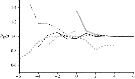
In the analysis below for each pandemic wave, the estimates for R_E and γ that arise from the fitting procedure converge to fixed values, denoted by ρ and Γ respectively, which for the relevant waves are shown in Table 1. In Figure 1 we show the convergence for R_E/ρ (which should tend to 1) with time (in weeks) either side of the week of maximum prevalence, given as 0 centred on the x-axis. For the 1957 and 1968–1969 outbreaks, R_E and γ approach to within 10% of ρ and Γ 2 weeks before the maximum influenza incidence for each wave. The 1918 waves behave a little differently. The first wave was very short and was only able to be fitted just as peak prevalence was occurring, which was also confounded due to data being unavailable for weeks prior to those shown (Fig. 4). Therefore, we report the final MLE prediction in the absence of converging behaviour. The second wave of the 1918 pandemic converged to a steady solution (±10% of subsequent estimates) 3 weeks before the peak. Interestingly, incorporating data for further weeks starts to break this convergence; this is because of a shoulder in the reported epidemic curve’s tail and so in Table 1 we report the estimates based on fitting to the weeks up to and including maximum prevalence. The third wave does not converge as convincingly to an obvious steady value (but still within ±10% of subsequent estimates) and so we use the parameters arising from the fit to 10 weeks of data. The values reported in Table 1 are consistent with those reported elsewhere [7].

Table 1.

Converged maximum likelihood estimators for the key epidemiological parameters in each pandemic wave

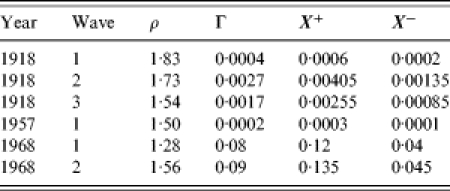
Fig. 1.

Figure showing R_E/ρ from the model as more data is incorporated. The x-axis shows the distance from the week of maximum prevalence. Solid black line: 1968–1969 first wave; dashed black line: 1968–1969 second wave; dotted black line: main wave 1957; solid grey line: 1918–1919 first wave; dashed grey line: 1918–1919 second wave; dotted grey line: 1918–1919 third wave.

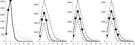
Fig. 4.

Figure showing the first wave of the 1918–1919 influenza pandemic with modelled projections (lines and symbols as in Fig. 2). Week 0 corresponds to the week ending 25 June 1918.

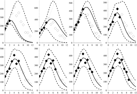
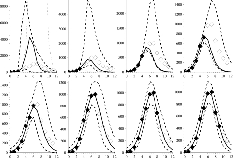
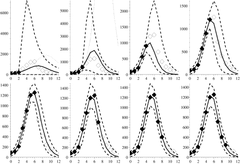
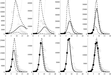
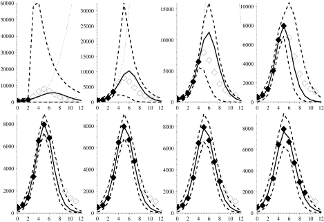
Figures 2–7 show the predicted epidemic curves for each pandemic wave where the known incidence data used to derive the relevant fit is represented by solid diamonds with the unknown future incidence shown as empty diamonds for comparison of the derived fit. The x-axis in each panel shows the number of weeks elapsed since the first rate used in the model was reported. Dotted lines appear in these Figures and represent the results of the method with the formal bound (0<γ⩽1). The unreliability of these curves in the early stages of an outbreak is because the model-derived value of γ is unrealistic in these situations. In the event of a new pandemic, sero- and other community-based epidemiological surveys (e.g. reporting behaviour and ILI symptoms) carried out rapidly at the earliest opportunity during the outbreak, both at home and abroad, would provide the required estimates to more reliably bound γ. As a surrogate for such data we use the derived values of Γ from Table 1. We amend our estimate of the behaviour of the limiting values on γ so that the limits are X^±=(1±0·5)Γ, as shown in Table 1, and note that we have intentionally placed a large error on γ of 50% because we are assuming the value. We would anticipate that the statistical analysis of epidemiological investigations in a future outbreak would make the error around this parameter smaller than this. The solid curve in each panel shows the MLE arising from placing such constraints on γ whilst the dashed curves reflect the envelope of potential epidemic trajectories that also fit the available data within a 95% credible interval given the constraint X^±=(1±0·5)Γ. In panels where no dotted curve appears it is coincident with the solid curve.

Fig. 2.

Figures showing the first wave of the 1968–1969 influenza pandemic with modelled week on week projections arising from fitting procedure. Solid diamonds: known incidence; open diamonds: future prevalence rates (currently unknown); solid curve: the optimal bounded MLE fit; dashed lines: 95% credible intervals on epidemic curve trajectories; dotted line: best formal MLE fit (in panels where no dotted curve appears it is coincident with the solid curve). Week 0 corresponds to the week ending 3 January 1969.

Fig. 7.

Figure showing major wave of 1957–1958 influenza pandemic with modelled projections (lines and symbols as in Fig. 2). Week 0 corresponds to the week ending 31 August 1957.

Hong Kong influenza pandemic: 1968–1970

The pandemic that initially struck the United Kingdom in 1968 exhibited two waves. The ILI data show that the first wave initially increased slowly producing only a weak signal and we delay fitting the model until the observed weekly rate is above 200 cases/100 000 population and has increased for three consecutive weeks.

Figure 2 shows the model fitted to the first wave of this pandemic. The three left-most panels in the top row of Figure 2, which correspond to fits to the first 3, 4 and 5 weeks of data respectively, all contain dotted curves showing the formal MLEs for the epidemic curve. We see that for 4 and 5 weeks of data the prevalence rates from the formal MLE eventually exceed the maximum plotted rate in each panel and thus considerably overestimate future prevalence. The fit to just 3 weeks of data has a very small standard error (s_e*∼7·8×10⁻³) associated with it and considerably underestimates future incidence. In the remaining panels the formal MLE (dotted curve) coincides with the solid line for the bounded MLE defined below.

Using data from Fleming et al. [26, and references therein] we find that the average RCGP reporting rate for ILI in seasonal influenza is ∼1/10 cases, giving an independent estimate of γ in the order of 0·1. From Table 1 we see that Γ=0·08, so whilst this model-derived value is more contemporary to this outbreak than the independent estimate from the literature, they are nonetheless close.

Therefore, based on the MLE with the more reasonably bounded γ we observe, in all the panels of Figure 2, that the envelopes around the weekly updated predicted epidemic curves encompass all but one future observation of the actual weekly prevalence right to the end of the pandemic wave. In addition, the one observation that falls below the lower bound of the envelope (Fig. 2: panel three, top row) does so only marginally. The predictions that are constrained by the more biologically feasible ranges for γ therefore appear to provide reasonable bounds within which to predict the future course of the epidemic and the envelopes become tighter as more weeks of data become available. This is despite the fact that this is only a relatively minor pandemic wave. The maximum prevalence is, for example, of a similar magnitude to the previous year’s seasonal influenza activity, with a maximum of only around 400 cases/100 000 population per week compared to over 1200/100 000 in the second wave of the 1969 pandemic (cf. Fig. 3).

Fig. 3.

Figures showing the second wave of the 1968–1969 influenza pandemic with modelled projections (lines and symbols as in Fig. 2). Week 0 corresponds to the week ending 21 November 1969.

The second pandemic wave occurred in 1969 and the results of the model for this wave are shown in Figure 3. Again, we see the pattern of over- or under-estimation during the early stages of the pandemic when we rely upon the formal MLE (dotted curves in panels reflecting results of fitting to 3 and 4 weeks of data and coincident with the solid curves in all other panels). Using the relevant values of X^± shown in Table 1 we derive our bounded MLE. Again the derived value of γ is in good agreement with the combination of reporting rate of community ILI cases and proportion of asymptomatic cases discussed above [26]. With the assumption of the bounds on γ the predictions estimate observed future incidence reasonably well, and much improve estimates of the timing of the maximum prevalence rate, which are correct to within 1 week. The reported value for week 11 in the last two panels in Figure 2 (based on 9 and 10 weeks of data) falls outside the MLE envelope. However, this is again marginal and we are well past the peak rate and at a level that would be considered normal seasonal behaviour.

Spanish influenza pandemic: 1918–1919

The 1918 pandemic occurred in three waves. No prior assumptions were made concerning case-fatality rates (γ) in this analysis. Further, we have no prior reliable estimate of R_E, particularly since some cases will have been subclinical. As stated above we require epidemiological studies to assist the bounding of parameter space and we use the values of γ given in Table 1in lieu of these studies. Given γ the envelope of feasible solutions (dashed curves) are derived.

For the first pandemic wave (see Fig. 4), the formal MLE happens to coincide with the constrained MLE in each situation. The modelled epidemic curves all predict the correct timing of maximum mortality and offer reasonable predictions for forthcoming weeks with the exception of the fit to the first 3 weeks of data, where the standard error of the MLE is very small and so the envelope of feasible fits is indistinguishable from the solid line. The model requires at least three data-points and it is unfortunate for fitting the model that earlier data are missing and after only 3 weeks we are at the peak for this wave.

Figure 5 shows the second wave of influenza to attack during 1918, which had much higher weekly mortality than the earlier wave. First, if we look at the formal MLE to 3, 4 and 5 weeks of data then we see gross overestimates for the eventual magnitude of the outbreak (dotted curves), despite short-term predictions for the next week being sound in each case. Even with the relevant bound on γ the MLE arising from 3 and 4 weeks of data (solid lines) does not provide good estimation of subsequent weeks’ mortality; this is because the influenza signal in the data is not strong enough at this time. However, the upper dashed 95% credible envelope does still capture most of the future weeks’ observed data and captures the timing of the peak of the signal. Output arising from fitting to 5–9 weeks of data converges to a small region of parameter space, hence the proximity of the envelope to the MLE.

Fig. 5.

Figure showing the second wave of the 1918–1919 influenza pandemic with modelled projections (lines and symbols as in Fig. 2). Week 0 corresponds to the week ending 14 September 1918.

However, the envelope from the fit to 9 weeks of data does not capture incidence in week 10 quite as well as previous fits. This is because a shoulder appears on the downslope of the outbreak curve, which may reflect a co-circulating epidemic variant of influenza or perhaps some spatial or age heterogeneity in the behaviour of the epidemic [4]. Simple mass-action models, like the one presented here, are not able to capture such behaviour in the epidemic curve, unless these features are well understood and can be parameterized ahead of time. We can fit, but not predict in advance, this shoulder by filtering out the main signal (if we assume the fit to 9 weeks of data has captured this signal), and then we find R_E=1·82 for this shoulder. Such a mathematical process is possible but its biological relevance, and practicality, during analysis of an outbreak is debatable because of the extra parameterization and data required.

Figure 6 show the results from our analysis of the third wave of the 1918–1919 pandemic. We observe that the formal MLE (dotted curves) for the fit to 3, 4 and 5 weeks of data over-predicts actual mortality. However, the bounded MLE in each panel provides a useful estimate of future prevalence until the tail of the pandemic curve is reached. Indeed the bounded estimates based on limited data (3, 4 and 5 weeks) only overestimate the timing of maximum prevalence in each case by 1 week.

Fig. 6.

Figure showing the third wave of the 1918–1919 influenza pandemic with modelled projections (lines and symbols as in Fig. 2). Week 0 corresponds to the week ending 25 January 1919.

Asian influenza pandemic: 1957–1958

Figure 7 shows the recorded deaths in England and Wales ascribed directly to influenza from the end of August 1957, and captures the main wave of the pandemic [5]. It takes 7 weeks of data before the formal MLE equates to the bounded MLE. The formal fit to 3 weeks of data results in a large overestimate of subsequent prevalence while interestingly the fits to 4, 5 and 6 weeks all underestimate subsequent prevalence. This is because the data behaves in such a manner that the formal MLE has an unrealistically low value for the optimal γ. The bounded MLE and the envelope around its 95% credible solution space, however, provide considerably better and more useful predictions for the future course of the pandemic.

SUMMARY

All of our derived bounded MLEs and associated potential solution envelopes are reasonable predictors of future prevalence rates and are much better than empirical judgements based purely on experience. Table 2 supplements Figure 1 and shows some summary measures of fit for each pandemic wave based on predictions from 4 and 5 weeks of data. The relative error in the amplitude of the peaks is simply the ratio of eventual peak incidence in the data and the predicted peak incidence from the model, which should tend to unity as the fit improves. We see, in the worst case, amplitude correctly predicted to within 50%, but more usually to within 20%. This is considerably better than relying on past experience, where, based on the pandemic waves illustrated here, actual amplitudes have varied by almost 300% (the two Hong Kong pandemic waves) and 550% (first wave of 1918 compared with the second wave 1918 pandemic). Table 2 also shows that we may draw conclusions regarding the timing of the peak of a pandemic wave [within ±1 week with RCGP data, −2 to +1 weeks with mortality data (+3 on one occasion)], again an improvement on using expectations from historical pandemic data, where time to peak from initial increase has varied from 3 to 9 weeks. Finally, predictions of epidemic duration are reasonable, being within 2 weeks of actual duration for RCGP reports (1968–1969) and −1 to −4 weeks for mortality data (1957, 1918). [Epidemic duration here being defined as the number of weeks that the RCGP ILI rates exceed 200/100 000 per week, or mortality exceeds 500 deaths per week (1918–1919) or 200 deaths per week (1957)], the thresholds for mortality data being arbitrarily chosen in these cases to facilitate their consistent application to the data at both ends of the pandemic. This compares well to simple expectations from previous pandemics which, for the thresholds given above, have varied from 6 to 16 weeks.

Table 2.

Summary information regarding fits to data

DISCUSSION

The purpose of a model such as the one described here is to assist public health officials reassess ongoing disease burdens and related resource allocations and realign contingency plans whilst a pandemic is in progress. Its purpose is not to replace existing contingency plans, which should be sufficiently robust and flexible to accommodate a range of likely scenarios and be in place ahead of time.

The model makes several assumptions in the way it is applied. It is assumed for example that the data recording influenza prevalence will be regularly and consistently reported, although we observe that the burden on GPs and other public health professionals to provide data at the same time as providing the necessary care for their patients may be great and data collection schemes could break down or become less reliable as a result. It is also presumed that case definitions remain the same throughout the outbreak and any lags between cases appearing in the community and those cases being assimilated into the data streams remain broadly constant. Such assumptions would apply to any similar statistical fitting procedure, unless the changes in reporting behaviour can be quantified and accommodated by the model. We also assume prior knowledge of the disease parameters (i.e. the duration of the latent and infectious periods) from independent epidemiological studies. The model here also fundamentally depends on the epidemic signal arising from the data conforming to a curve arising from a homogeneous mixing mass-action framework. Should heterogeneity in the mixing become a dominant feature, be it spatial, demographic or strain dependent the model will become less reliable. That is, unless the model is adjusted by the incorporation of further parameters (such as age-structured mixing) and that these parameters can be reliably and independently assessed or fitted by statistical procedures.

Furthermore, forecasts would be weakened if public health interventions were initiated (or removed) midway through a pandemic since the method assumes a constant basic reproduction number. However, in this situation the method could be used in some instances to measure the effectiveness of said interventions. If interventions were put in place before a clear signal appeared in the reported data, and remained equally effective throughout, their effect would be implicitly incorporated into the model-derived reproduction number and the estimates of future incidence would remain valid. If the timing of new or escalated interventions was known they would be expected to coincide with deviations from the ‘ideal’ behaviour and should also become obvious from the fitting procedure.

Nonetheless, we have shown that statistical fitting of a simple mass-action compartmental-type model did predict future measures of pandemic influenza incidence reasonably well, but only if sensible bounds were placed on key input variables, particularly at the beginning of pandemic waves. In the examples shown here, the formal MLE prediction (dotted curves in each figure) did require less epidemiological data ahead of time than the constrained MLE approach but also needed more (4–6) weeks of data before it matched the trajectory of the subsequently observed data fairly well. It is clearly important, therefore, that in-depth epidemiological studies are performed early in the pandemic to attempt to independently estimate the parameters needed to bound the fitting process, as the formal unbounded MLE will be unreliable for producing early predictions. The relatively infrequent individual weekly reports that lay outside the envelope of our fits were consistently in the tail of the epidemic. The fact that the tails of each wave were not well captured by the model may be due to a range of factors, including heterogeneous mixing in the population. However, for the purposes of the problems being addressed here the fitting of these tails is of much less consequence than in other types of epidemic modelling applications.

As stated previously, more complex models incorporating demographic heterogeneities could be developed if they could be adequately parameterized. Further, if available, multiple surveillance data streams should be analysed to provide consistency checks and more robust estimates from the output derived. We would hope, for example, that for the next pandemic in the United Kingdom, NHS direct data, RCGP reports and ONS mortality records would all be available and able to be used concurrently [27]. More frequent observations than weekly reports might also be expected to improve the results particularly in the early few weeks of a pandemic (i.e. 3 or 4 weeks), but only if observational errors are not amplified in the data in tandem with the more frequent reporting. Indeed, some of the reporting schemes identified above may well be enhanced to provide daily or twice weekly reports for a future pandemic.

APPENDIX. Data analysis and modelling

Data

Let us assume that the observable symptomatic case-incidence data is constructed in the following manner

where, at a reporting point w we find is the true infected (and assumed infectious) case incidence rate, r_W is a normally distributed random variable with mean zero and constant variance σ_A, whilst η reflects the relationship between the data source and the population. For example, the RCGP provides weekly reporting rates and so η in this situation would be the probability that an infected case reports to their GP. If the data showed the hospitalization rate during an outbreak then η would be the probability that an infected case is admitted to hospital.

Further noise is allowed in the data through the mean seasonal number of mistaken records . Away from a pandemic wave, we assume whilst the mistaken records are assumed constant (although not necessarily the same value either side of the epidemic window, nor the same value from year to year; whilst GP consultations appear to have decreased over a long timescale the precise behaviour of is beyond the scope of this study). During a sizable influenza outbreak we assume misdiagnosis is negligible () and so for simplicity we allow , although we intend to explore the validity of this assumption in future work). The period between each report is τ_R days.

We assume deaths from influenza occur some time (which is fitted, see later) after a loss of infectiousness and so a case that results in death will be reported after they were recorded as a case. Such observed deaths D, are assumed to take the form

where represents the expected reported deaths with δ, the proportion of infected cases that die and subsequently get recorded in the data and d_w is the weekly error between the actual and expected epidemic curves. In the analysis, some datasets will reflect only deaths directly attributed to influenza whilst others will include probable influenza deaths due to pneumonia and other complications also. Mistaken identification of cause of death is assumed proportional to the number of reported deaths and thus implicit in the definition of δ.

Model

Given the two basic forms of potential data (some scaling of cases or a scaling of recovered cases) we build a model with the flexibility to accommodate either example. Therefore, we formulate a deterministic mass-action model [21] incorporating latency, E, asymptomatic contagiousness, A, and then symptomatic contagiousness, I, into three separate classes along with susceptible, S, and recovered, R, populations. A case is typically assumed latent for τ_E days, asymptomatic for τ_A days and symptomatic for τ_I days before recovery. We assume a constant population (outbreak timescale is less than lifespan of humans) with some fraction of the population attacked by the disease and so our equation of state becomes S+E+A+I+R=φN where φ is a measure of the background immunity of the population prior to onset of the disease transmission through the population at large.

We have initial conditions S(0)=S_fφN, E(0)=E_fφN, A(0)=A_fφN, I(0)=I_fφN and R(0)=0, where X_f denotes the fraction of the population in each subset. To simplify our future analysis of parameter space we consider an epidemic arising from a fixed proportion of the susceptible population becoming instantaneously infected, so E_f=(φN)⁻¹ while A(0)=I(0)=R(0)=0 and S_f=1−E_f.

We may normalize the populations about the number susceptible at onset S_fφN and we set the natural timescale of the model to match the reporting period τ_R then the system is governed by the following set of equations (reusing notation where appropriate):

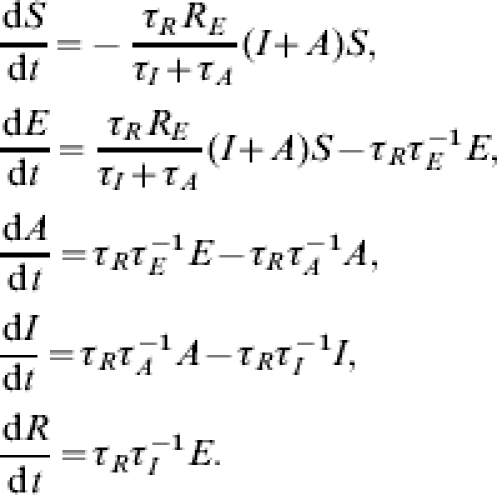The parameter R_E is the effective reproduction number; the average number of secondary cases expected from an index cases given the potential susceptibility level S_fφ. The basic reproduction number through a virgin population is given by R₀=R_E/(S_fφ). We assume that individuals are equally infectious during asymptomatic and symptomatic infectious periods.

If we consider the possible scaling of ILI-reporting data then we assume the earliest of the data records to be fitted occurs τ_S days from the contrived initial situation. We also assume that all the people that report to a doctor do so upon developing symptoms, then in the SEAIR framework, I^A is given by the integral of between reporting periods. If we set

where w∊ℕ₀ then we have . The assumption that misdiagnosis is negligible during the major part of a pandemic wave means we may define

with M, the number of weeks of observations under consideration and γ =ηφ∊(0,1).

For a number of observations, M, we minimize Δ by adjusting the parameters in the problem and in doing so derive the MLE for the pandemic prevalence rates. However, some of the parameters can be measured or estimated prior to an outbreak and so may be treated as constants in the problem. For example, τ_R and N are definitely known ahead of time and are dependent on the data stream under consideration, whilst the initial import 1−S_f is fixed. The disease kinetics τ_E, τ_A, τ_I will be drawn from the literature and opinion discussed above, whilst in the event of a response to a new pandemic these parameters would be re-evaluated based on the tests carried out in countries that have already experienced the disease. Of the remaining parameters, γ limits eventual prevalence rates that are measured in the community and is formally a number between 0 and 1, with its biological significance dictated by the data under consideration. The phase shift τ_S is only of academic interest, due to the contrivance in the initial conditions, we constrain this such that, 0⩽τ_S<τ_Smax (otherwise the epidemic would be allowed to start after the first few cases were observed in this country or before they were noted abroad). The critical unknown in the problem is thus R_E the reproduction number through the population at the start of the pandemic wave. This may be estimated from other countries and data but it is likely to vary across social scales, as it is dependent on contact rates. We should note that the reproduction number and disease kinetics can be written as a function of the invariant exponential growth rates at the start and end of an outbreak allowing some simple sensitivity analysis about the disease timescale. Therefore we find the minimum of Δ subject to R_E, τ_S and γ and treat all other parameters as predetermined constants.

We will thus have a set of parameters R_E=ρ, τ_S=τ_Smin, γ=X that correspond to the global minimum of Δ, and this set provides us with the MLE for the true epidemic parameters. Observe that γ is conditionally linear in Δ, thus given arbitrary values of R_E and τ_S we find the value for γ that minimizes Δ will be

and hence the global minimum value is given by X=γ_min(M, ρ, τ_Smin). However, γ is a probability and so formally may not exceed unity; we shall further constrain the value of γ based on available epidemiological studies carried out during the early stages of a new pandemic to find the reporting rate, etc., and so 0⩽X⁻<γ⩽X⁺⩽1.

We define the minimum standard error of the system s_e*=Δ_min/(M – 2) where Δ_min=Δ(M, ρ, τ_Smin), the global minimum of Δ. The standard error is an estimate of the standard deviation of the systems residuals r_w, and so we set s_t=t_{(0·05, M−2)}s_e* [where t_{(0·05, M−2)} is taken from an inverse t-distribution]. A crude measure of parameter deviation is provided by allowing any set of parameters with standard error such that s_e<s_t to be a potential solution (i.e. within 95% of the optimal solution). We thus define ŝ_e=s_e/s_t and so for a given number of weeks of observations M we admit epidemic curves to be potential solutions if ŝ_e(R_E, τ_S)<1. Furthermore, having found the global minimum Δ_min, for an arbitrary choice of R_E and τ_S we may find the closed form for feasible values of γ. Should such values exist their range will be bounded by,

otherwise, where

Of course if γ_lim∊ℂ for R_E and τ_S then the chosen coupling results in a standard error outside of potential solution space. Therefore, given values for the phase shift and reproduction number we may solve for γ completely and it is separated from the problem.

Provided with estimates of the infected case-fatality rate and the delay between infection and reporting of influenza-related death, we may also predict the number of deaths likely to occur in each future week. Death will obviously occur some point after infection and for simplicity in this analysis we assume that deaths will occur to cases in our population R, and so new deaths over a given week will be given by

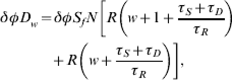where Δ is a parameter incorporating the case-fatality rate for the particular strain of influenza and allowance for underreporting, whilst τ_D is the delay between loss of infectiousness and the recording of death, both of which may be available from studies in countries that have already experienced the virus and from such studies carried out very early in the influenza-affected country in question.

If we are attempting to fit the model to a scaling of reported recovered cases then, . However, rather than estimate δ and τ_D we may allow Δ to take the form

where and , although for brevity in the main body of the text the hat notation will be dropped. The same process to that discussed above for minimizing Δ for GP ILI-reporting data may then be followed.

DECLARATION OF INTEREST

None.

REFERENCES

- 1.Nguyen-Van-Tam JS, Hampson AW. The epidemiology and clinical impact of pandemic influenza. Vaccine. 2003;21:1762–1768. doi: 10.1016/s0264-410x(03)00069-0. [DOI] [PubMed] [Google Scholar]
- 2.Kilbourne ED. Influenza pandemics of the 20th century. Emerging Infectious Diseases. 2006;12:9–14. doi: 10.3201/eid1201.051254. [DOI] [PMC free article] [PubMed] [Google Scholar]
- 3.Taubenberger JK, Morens DM. 1918 Influenza pandemic. Emerging Infectious Diseases. 2006;12:15–22. doi: 10.3201/eid1201.050979. [DOI] [PMC free article] [PubMed] [Google Scholar]
- 4.Ministry of Health Reports on Public Health and Medical Subjects1920
- 5.Ministry of Health. 1960.
- 6.Meltzer MI, Cox NJ, Fukuda K. The economic impact of pandemic influenza in the United States: priorities for intervention. Emerging Infectious Diseases. 1999;5:659–671. doi: 10.3201/eid0505.990507. [DOI] [PMC free article] [PubMed] [Google Scholar]
- 7.Gani R et al. Potential impact of antiviral drug use during pandemic influenza. Emerging Infectious Diseases. 2005;11:1355–1362. doi: 10.3201/eid1109.041344. [DOI] [PMC free article] [PubMed] [Google Scholar]
- 8.Serfling RE. Methods for current statistical analysis of excess pnuemonia-influenza deaths. Public Health Reports. 1963;78:494–506. [PMC free article] [PubMed] [Google Scholar]
- 9.Costagliola D et al. A routine tool for detection and assessment of epidemics of influenza-like-illness. American Journal of Public Health. 1991;81:97–99. doi: 10.2105/ajph.81.1.97. [DOI] [PMC free article] [PubMed] [Google Scholar]
- 10.Toubiana L, Flahault A. A space-time criterion for early detection of epidemics of influenza-like-illness. European Journal of Epidemiology. 1998;14:465–470. doi: 10.1023/a:1007481929237. [DOI] [PubMed] [Google Scholar]
- 11.Carrat F, Valleron AJ. Epidemiologic mapping using the kriging method: application to an influenza-like-illness epidemic in France. American Journal of Epidemiology. 1992;135:1293–1300. doi: 10.1093/oxfordjournals.aje.a116236. [DOI] [PubMed] [Google Scholar]
- 12.Viboud C et al. Prediction of the spread of influenza epidemics by the method of analogues. American Journal of Epidemiology. 2003;158:996–1006. doi: 10.1093/aje/kwg239. [DOI] [PubMed] [Google Scholar]
- 13.Quenel P, Dab W. Influenza A and B epidemic criteria based on time-series analysis of health services surveillance data. European Journal of Epidemiology. 1998;14:275–285. doi: 10.1023/a:1007467814485. [DOI] [PubMed] [Google Scholar]
- 14.Hashimoto S et al. Detection of epidemics in their early stage through infectious disease surveillance. International Journal of Epidemiology. 2000;29:905–910. doi: 10.1093/ije/29.5.905. [DOI] [PubMed] [Google Scholar]
- 15.Mooney J, Wright E, Christie P. Predictive modelling of influenza outbreaks: a linear regression analysis. SCIEH Weekly Report. 2001;35:134–135. [Google Scholar]
- 16.Elveback L et al. Stochastic two-agent epidemic simulation models for a community of families. American Journal of Epidemiology. 1971;93:267–280. doi: 10.1093/oxfordjournals.aje.a121258. [DOI] [PubMed] [Google Scholar]
- 17.Le-Strat Y, Carrat F. Monitoring epidemiological surveillance data using hidden markov models. Statistics in Medicine. 1999;18:3463–3478. doi: 10.1002/(sici)1097-0258(19991230)18:24<3463::aid-sim409>3.0.co;2-i. [DOI] [PubMed] [Google Scholar]
- 18.Longini I, Fine P, Thacker S. Predicting the global spread of new infectious agents. American Journal of Epidemiology. 1986;123:383–391. doi: 10.1093/oxfordjournals.aje.a114253. [DOI] [PubMed] [Google Scholar]
- 19.Mills CE, Robins JM, Lipsitch M. Transmissibility of 1918 pandemic influenza. Nature. 2004;432:904–906. doi: 10.1038/nature03063. [DOI] [PMC free article] [PubMed] [Google Scholar]
- 20.Wallinga J, Teunis P. Different epidemic curves for severe acute respiratory syndrome reveal simila impacts of control measures. American Journal of Epidemiology. 2004;160:509–516. doi: 10.1093/aje/kwh255. [DOI] [PMC free article] [PubMed] [Google Scholar]
- 21.Anderson RM, May RM. Infectious Diseases of Humans. Oxford University Press; 1992. [Google Scholar]
- 22.Flauhault A et al. Modelling the 1985 influenz epidemic in France. Statistics in Medicine. 1988;7:1147–1155. doi: 10.1002/sim.4780071107. [DOI] [PubMed] [Google Scholar]
- 23.Davis DJ et al. Epidemiological studies on influenza in familial and general population groups, 1951–1956, III laboratory observations. American Journal of Hygiene. 1960;13:138–147. doi: 10.1093/oxfordjournals.aje.a120172. [DOI] [PubMed] [Google Scholar]
- 24.Fleming D. Weekly returns service of the Royal College of General Practitioners. Communicable Disease and Public Health. 1999;2:96–100. [PubMed] [Google Scholar]
- 25.Goddard NL, Kyncl J, Watson J. Appropriateness of thresholds currently used to describe influenza activity in England. Communicable Disease and Public Health. 2003;6:238–245. [PubMed] [Google Scholar]
- 26.Fleming D, Zambon M, Bartelds A. Population estimates of persons presenting to general practitioners with influenza-like illness, 1987–96: a study of the demography of influenza-like illness in sentinel practice networks in England and Wales, and in The Netherlands. Epidemiology and Infection. 2000;124:245–253. doi: 10.1017/s0950268899003660. [DOI] [PMC free article] [PubMed] [Google Scholar]
- 27.HPA website.http://www.hpa.org.uk/infections/topics_az/influenza/seasonal/uk_data_sources.htm