Influence of the transmission function on a simulated pathogen spread within a population

T HOCH; C FOURICHON; A-F VIET; H SEEGERS

doi:10.1017/S095026880700979X

. 2007 Dec 6;136(10):1374–1382. doi: 10.1017/S095026880700979X

Influence of the transmission function on a simulated pathogen spread within a population

T HOCH ^1,^*, C FOURICHON ¹, A-F VIET ¹, H SEEGERS ¹

PMCID: PMC2870731 PMID: 18062825

SUMMARY

The mathematical function for the horizontal transmission of a pathogen is a driving force of epidemiological models. This paper aims at studying the influence of different transmission functions on a simulated pathogen spread. These functions were chosen in the literature and their biological relevance is discussed. A theoretical SIR (Susceptible–Infectious–Recovered) model was used to study the effect of the function used on simulated results. With a constant total population size, different equilibrium values for the number of infectious (NI) were reached, depending on the transmission function used. With an increasing population size, the transmission functions could be assimilated to either density-dependent (DD), where an equilibrium was obtained, or frequency-dependent (FD), with an exponential increase in NI. An analytical study corroborated the simulated results. As a conclusion, the choice between the different transmission functions, particularly between DD and FD, must be carefully considered for a varying population size.

INTRODUCTION

Modelling approaches, which allow, among other uses, the simulation of different scenarios of management and control, are widely used in epidemiology, whether applied to human or animal diseases [1–3]. Mathematical models representing the pathogen spread use a function to represent the horizontal transmission of this pathogen between the hosts of a population. This transmission function can be considered the driving force of many epidemiological models and great attention must be paid to its mathematical formulation [4, 5].

Despite the recognized influence of the transmission function in models, many papers, even those dealing with the same pathogen, use different mathematical forms without eliciting the underlying assumptions or detailing the reasons for their choice. Some papers gather and study different transmission functions encountered in models [5, 6]. However, no work has been dedicated to the influence of the transmission function on the results of an epidemiological model.

The objective of this paper was to assess the effect of different transmission functions on the results of pathogen-spread simulations in a population. First, this paper will describe the different transmission functions encountered in the literature in continuous-time models. We examined more particularly the assumptions underlying the choice of a given transmission function, when available. Second, the influence of different transmission functions on simulation results was investigated for a theoretical model, through a well-known SIR (Susceptible–Infectious–Recovered) type model. This influence was assessed first thanks to a simulation study and then by exploring analytical results from the model.

TRANSMISSION FUNCTIONS: DEFINITION AND MATHEMATICAL FORMS

The following sections are largely inspired by Begon et al. [5].

Definition

The horizontal transmission of a pathogen is defined as the spread of this pathogen between hosts after birth. Only transmission by direct contact was considered here.

From Begon et al. [5], a convenient way to define horizontal transmission is to consider a system formed by the number of Susceptible (S) and Infectious (I) hosts. Horizontal transmission is represented by the interaction term between S and I and may be formulated as follows in a continuous-time model:

${{{\rm dI}} \over {{\rm d}t}} \equals {\rm S}cp\eta \comma\hfill$

(1)

The rate of increase in the number of infectious hosts, namely the force of infection, is represented by the product cpη, where c is the contact rate (in t⁻¹), p represents the probability that this contact occurs with an infectious host and η is the probability of successful transmission. Usually, p is estimated by the ratio I/N (N=population size) and η is considered constant for a given host–pathogen system. The value of the force of infection, and therefore of the transmission function, is thus determined by the expression of the contact rate c.

Mathematical forms

Continuous-time models

Depending on the mathematical formulation for the contact rate c, different forms of the transmission function may be deduced. Two main cases encountered in the literature are considered:

c varies linearly with the density of hosts, c=κN/A (A=area occupied by the population). With β=κη, one obtains the following equation:
${{{\rm dI}} \over {{\rm d}t}} \equals \beta {\rm S}{{\rm I} \over A} \comma$ (2)
This transmission function corresponds to the density-dependent (DD) form. When A is considered constant, changing β to β′ in equation (2) leads to the following equation:
${{{\rm dI}} \over {{\rm d}t}} \equals \beta ^\prime{\rm SI}.$ (3)
c is constant, c=τ, and considering β′=τη, equation (1) becomes:
${{{\rm dI}} \over {{\rm d}t}} \equals \beta ^{\prime\prime} {\rm S}{{\rm I} \over N}.$ (4)

This equation is often called the frequency-dependent (FD) form, since I/N might be termed the frequency of infectious hosts. As suggested by Begon et al. [5], we chose to use further on in this paper the terms ‘DD’ and ‘FD’, as representative of the underlying biological processes, rather than other terms found in the literature.

In the DD form, the assumption of a linear increase in the contact rate with the density of hosts often seems realistic, but when the density of organisms becomes high, this increase may be limited by a saturation phenomenon [7].

The FD form is usually applied to sexually transmitted diseases [6], where the contact rate depends more on the mating system of the species than on the density of the population.

From Begon et al. [5], a DD form is often applied to a homogeneous contact structure whereas a FD form is often used when the contact structure is heterogeneous. However, the respective associations between the form of transmission function, either DD or FD, and the homogeneous or heterogeneous contact structure are not exclusive. More generally, the transmission function must be adapted to a particular host–pathogen system.

Within the same model, the spread of a pathogen in a population may be represented by these two forms of transmission function. Fromont et al. [8], in a study on the spread of a feline retrovirus, used different definitions for the contact rate between domestic cats, depending on their population density. In that paper, the contact rate was constant at low densities of hosts, on account of the infrequency of encounters between hosts. For intermediate densities, the contact rate was either proportionate to the density, or constant for higher densities because of the reduction in the size of the territory in rural or suburban areas. When densities became high in urban areas, the contact rate increased once again proportionately to the host density, since animal territories overlapped. The formulation of the contact rate and of the related transmission function depended in that case on the variable spatial structure of cat populations.

Apart from DD and FD transmission functions, other mathematical forms have been developed and used, either in theoretical or in applied studies.

As for theoretical approaches, which mainly focus on model behaviour, Hochberg [9], inspired by the initial DD form, introduced a nonlinear transmission coefficient:

$\hat{\beta } \equals \beta \left[ {{\rm S}^{p} {\rm I}^{q} } \right]{\rm SI} \comma\hfill$

(5)

where p and q represent the way the density of susceptible and infected hosts may respectively affect per capita transmission efficiency (−1⩽p⩽+1 and so for q). Depending on the values for p and q, different hypotheses underlying the model may be expressed (acceleration or deceleration with densities, or even a negative response type). Hethcote & van den Driessche [10] studied the behaviour of epidemiological models in a case of nonlinear transmission. The force of infection uses the form βg(I), where g(I) is a function of the type I^r/(1+αI^s). Parameters r, s and α represent the way infectious hosts influence the force of infection. Different values for r, s and α allow the representation of different forms for the transmission function. For instance, with r=s=1, a saturation effect may be taken into account. For r=1 and α=0, the model is equivalent to the DD equation (3).

On the contrary, other transmission functions have been used in applied epidemiological models. For instance, using equation (3), the ‘refuge effect’ model takes into account an aggregation parameter h which decreases the number of susceptible hosts: βI(N – I/h). The aggregation parameter h represents the proportion of the population that is potentially susceptible, on account of spatial heterogeneities. This function equals zero when I⩾hN. This model was applied to the possum/bovine tuberculosis system in New Zealand [11].

The same author, working on the same system, used more recently a negative binomial type equation for the transmission function: kS ln (1+βI/k), with k a constant [12]. When k is low, the aggregation level is high and this implies a decrease in the mean number of infected animals per susceptible host. The choice of this function lies in the analogy with a host–parasitoid system. Such a model, termed ‘heterogeneous mixing’ by the author, reproduces more realistically the observed characteristics of the considered pathogen spread than a ‘homogeneous-mixing’-type model like density-dependence. It allows the simulation of the heterogeneity of risks related to the spatial patchiness of host density.

A saturation effect on the contact rate has been taken into account in different models [13–15]. For Diekmann & Kretzschmar [13], an asymptotic form of the transmission function may be used to account for this effect: βSI/(l+N), where l is a constant associated with this saturation effect.

INFLUENCE OF THE TRANSMISSION FUNCTION ON THE RESULTS OF A THEORETICAL SIMPLE MODEL

The model

To investigate the influence of different forms of the transmission function on the simulated results of a model, we first chose to use a classical theoretical SIR-type model, as described by Anderson & May [16]. In this first study, we focused on a continuous-time deterministic model, which has been much studied and is appropriate for theoretical and analytical approaches. This model had three state-variables: the number of Susceptible (S), Infectious (I) and Recovered (R) hosts. The area occupied by the hosts was considered constant and these state variables could be expressed either as numbers or as densities. Horizontal transmission governed the flux from S to I. The transitions between I and R, and R and S, occurred respectively at rates υ and γ. The three types of hosts gave birth to susceptible hosts S with the same birth rate a. Two cases were considered in the simulations: (i) when the population size N was constant, (ii) when the population might increase. In the former case, birth and mortality (b) rates were identical for all the state-variables (a=b). In the latter, a>b and an additional mortality rate μ due to the infection was applied to infectious hosts I. The model was represented by the following system of differential equations:

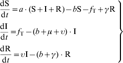$\left. \openup6{\matrix{ \displaystyle{{{{\rm dS}} \over {{\rm d}t}} \equals a \cdot \lpar {{\rm S} \plus {\rm I} \plus {\rm R}} \rpar \minus b{\rm S} \minus f_{\rm T} \plus \gamma {\rm R}}\hfill \cr {\displaystyle{{{\rm dI}} \over {{\rm d}t}} \equals f_{\rm T} \minus \lpar {b \plus \mu \plus \upsilon } \rpar \cdot {\rm I}} \hfill\cr {\displaystyle{{{\rm dR}} \over {{\rm d}t}} \equals \upsilon {\rm I} \minus \lpar {b \plus \gamma } \rpar \cdot {\rm R}}\hfill \cr} } \right\}\hfill$

(6)

where f_T represents the transmission function and Table 1 describes the different forms of the transmission functions considered in this analysis. These functions corresponded mostly to those detailed in the first part of this article. However, we chose to exclude the forms used in mathematical and theoretical studies, like those of Hochberg [9] and Hethcote & van den Driessche [10]. These functions were also difficult to include in such a comparative work, on account of their nonlinear forms, with too many parameters involved.

Table 1.

Transmission functions used in the different models

graphic file with name S095026880700979X_tab1.jpg

Open in a new tab

The area was considered constant. S and I represented the respective numbers of susceptible and infectious hosts and N the population size. The transmission coefficient β_i corresponded to model M_i. Its unit varies according to the transmission function considered.

Whatever the transmission function considered, the parameters a, b, μ, υ and γ had the same values: a=0·01 day⁻¹, b=0·01 (N constant) or 0·005 day⁻¹ (N variable), μ=0 or 0·01 day⁻¹, υ=0·05 day⁻¹ and γ=0·1 day⁻¹. Additional parameters were necessary for models M3 (h=0·6, no unit), M4 (k=0·1 ind⁻¹ day⁻¹ where ind means individuals) and M5 (l=50 ind). The spread of the infection was obtained by introducing an infectious host into a population of 99 susceptibles. The model was run using SciLab^© software (http://www.scilab.org).

In order to compare the five different models, the same basic reproductive number (R₀) was considered for all of them. This number represents the number of secondary infections caused by an infectious host during its infectious period, in a totally susceptible population. Following Lopez et al. [18] and Coutinho et al. [19], it can be obtained by considering S=N and I=R=0 in system (6) and by analysing the stability of this trivial solution. By linearizing this system around this solution, it becomes, with i deviating slightly from zero:

${{{\rm d}i} \over {{\rm d}t}} \equals f_{\rm T} \lpar i \rpar \minus \lpar {b \plus \mu \plus \upsilon } \rpar \cdot i.\hfill$

(7)

Around zero, f_T(i) can be approximated by:

$f_{\rm T} \lpar i \rpar \equals f_{\rm T} \lpar 0 \rpar \plus i{{{\rm d}f_{\rm T} \lpar 0\rpar } \over {{\rm d}i}} \plus {\rm o}\lpar {i^{\hskip1\setnum{2}} } \rpar .\hfill$

(8)

For the considered transmission functions, f_T(0)=0 and the condition for a spread of the infection (di/dt>0) leads to the following expression for R₀:

${R}_{\rm \setnum{0}} \equals {{{\rm d}f_{\rm T} \lpar 0\rpar \sol {\rm d}i} \over {b \plus \mu \plus \upsilon }}.\hfill$

(9)

In the case of the constant population size (N=100 ind), the following procedure was carried out. We fixed β₁, corresponding to model M1 (DD), at a value of 0·001 day⁻¹ in order for the infection not to die out. The corresponding R₀ equals 1·667 with the given parameter values. The other values for the transmission coefficient β (for models M2–M5) were calculated in order to have the same R₀ between models. Table 2 shows the different expressions in the β/R₀ relationship with the resulting values used later in this paper for the transmission coefficients.

Table 2.

Value and corresponding unit for the transmission coefficient β_i used in the different models (β_i corresponded to model M_i)

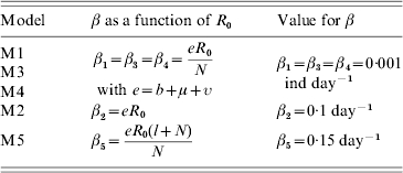
graphic file with name S095026880700979X_tab2.jpg

Open in a new tab

ind, Number of individuals.

β_i was calculated from R₀, whose value was fixed at 5/3 in the case of a constant population size. See text for parameter signification and value.

In the case of an increasing population size, the comparison was again based on the same value for R₀, calculated at the beginning of the simulation (i.e. with N=100 ind once again). We chose to keep the same values for the transmission rates as in the former case, which resulted in a slight decrease of R₀ (=1·538), on account of an increasing global mortality rate for the infectious hosts.

The M1–M5 models were compared first through the occurrence or the absence of equilibrium, by simulation. When equilibrium was simulated, the time to reach it, as well as the value then obtained for the number of infectious hosts and their proportion in the population, were also used to compare the different models. The duration of the simulations was adapted to the time required for equilibrium to be reached, in each case (constant or variable population size). Analytical studies were also carried out to complete these comparisons and corroborate the simulated results.

Simulation results

Constant population size

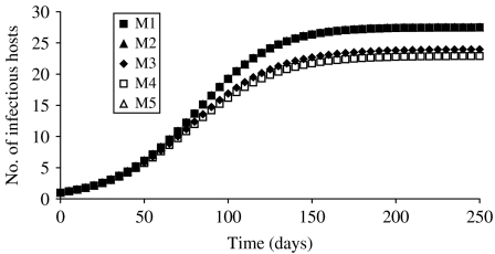
The evolution in the number of infectious hosts for the five transmission forms considered was plotted on Figure 1. By construction, DD, FD and asymptotic models (M1, M2 and M5) were identical. The value for the parameter transmission derived from Table 2 gave similar values for the different forces of infection in these cases. The shape of the curve was quite similar among the different models. The number of infectious hosts increased considerably at the beginning of the simulation before reaching equilibrium. Since R₀ was always the same for the different models, the simulated dynamics were identical at the beginning of the simulation. They differentiated thereafter but their equilibrium was reached at about the same time, i.e. before day 150, for all models. The equilibrium values reached by M3 and M4 (22·9 ind and 24·0 ind respectively) were lower than the values obtained with M1, M2 and M5 (27·5 ind). Due to the model type, decimal numbers were obtained. With a constant population size of 100 individuals, they were equivalent to the corresponding percentages. Even with a constant population size, differences in the behaviour of the models were therefore encountered in some cases, due solely to changing transmission functions.

Fig. 1 — Evolution in the number of infectious hosts simulated by the models M1–M5 corresponding to different forms of transmission functions. The population size was kept constant. By construction, M1, M2 and M5 were identical.

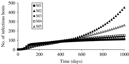
Variable population size

More differences between the models were highlighted when a population increase was simulated (Fig. 2). A longer simulation duration than in the case of a constant population (1000 vs. 250 days) was required in order to distinguish models which led to equilibrium and the others. More particularly, being diametrically opposed, the number of infectious hosts reached equilibrium for M1 whereas an exponential increase in infectious hosts was obtained with M2. The behaviour of the other models could be assimilated to one of these two cases: M3 and M4 reached equilibrium, but later than M1. With a longer simulation duration, M5 would also exhibit an exponential increase in the number of infectious hosts, although in an attenuated manner compared to M2.

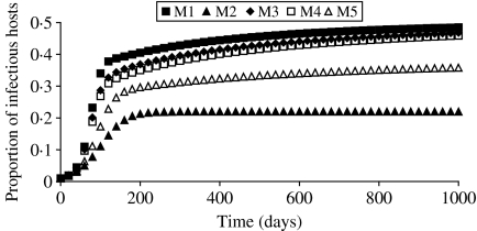
What was interesting was the evolution in the proportion of infectious hosts for the different models (Fig. 3). Whatever the transmission function and the corresponding model considered, all the proportions evolved to a stable value. This was due to an identical evolution in the number of infectious hosts and in the size of the population. The proportions of infectious hosts obtained with M1 and M2 at the end of the simulation were found on opposite ends from each other, and results from the other models were distributed in the same order between M1 and M2 as in Figure 2.

Analytical studies, equilibrium analyses

Some of the previously described results may be retrieved through an analytical study. Some have already been reported in the literature. For instance, Anderson & May [16] studied the same SIR model as ours, with a DD transmission function. The simulations presented in this paper for model M1 illustrate some of their results. From the system of equations (6), the evolution in the total population may be deduced from the following differential equation:

${{{\rm d}N} \over {{\rm d}t}} \equals \lpar {a \minus b} \rpar \cdot N \minus \mu \cdot {\rm I}\comma\hfill$

(10)

This equation simply illustrates the fact that the population size depends on the balance between birth and mortality, either ‘natural’ or due to the infection. From Anderson & May [1], the system of equations (6) evolves to an equilibrium when

$\mu \minus \lpar {a \minus b} \rpar \cdot \left( {1 \plus {\upsilon \over {b \plus \gamma }}} \right) \gt 0 \comma\hfill$

(11)

which is the case with our parameters. At equilibrium, prevalence I/N obviously equals (a – b)/μ, namely 0·5 in this paper with the considered parameter values.

In the case of a FD model (M2), we showed that the equilibrium depended not only on the same condition given by equation (11), but also on the value of the transmission coefficient β₂. By setting system (6) and equation (10) to zero, a positive equilibrium was obtained for the following value of the transmission coefficient:

$\beta_{\setnum{2}}\hskip-3 {\ast } \equals {{\mu \plus b \plus \upsilon } \over {1 \minus \displaystyle{{a \minus b} \over \mu } \cdot \left( {1 \plus {\upsilon \over {b \plus \gamma }}} \right)}}.\hfill$

(12)

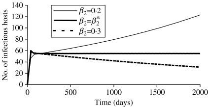
In our case, β₂* equalled 0·248 day⁻¹. For this value, I, N and the prevalence tended to reach a plateau, and its value for prevalence also equalled (a−b)/μ. If β₂ was higher than β₂*, the population became extinct. If the value for β₂ was below the threshold value β₂*, which was the case in this paper, the population and the number of infectious hosts increased exponentially. Figure 4 illustrates different model behaviours depending on the value of the transmission coefficient.

Fig. 4 — Influence of the value for the transmission coefficient (β₂) on the simulated number of infectious hosts for a model using a frequency-dependent form of the transmission function (M2). The value β₂* corresponded to the value necessary to reach equilibrium.

In our simulations, the prevalence simulated by the FD model M2 tended to reach a plateau, but at a lower value than the one reached by the DD model M1. We calculated the value reached with M2 by considering that equilibrium for prevalence was reached when:

${{{\rm d}\lpar {\rm I}\sol N\rpar } \over {{\rm d}t}} \equals 0 \Rightarrow {{\rm I} \over N} \equals {{{\rm dI}\sol {\rm d}t} \over {{\rm d}N\sol {\rm d}t}}.\hfill$

(13)

Similar equations to equation (13) were written for the proportions for S and R in the population. Moreover, the sum of the respective proportions for I, S and R obviously equalled 1. Solving these equations led to a second-degree equation for prevalence for which the sole solution between 0 and 1 was 0·218 with our parameters, which corresponded to the equilibrium prevalence for M2 (Fig. 3). Moreover, this second-degree equation always had solutions for a transmission coefficient value for which the infection spread, i.e. when β₂<β₂*, thus explaining the stable prevalence obtained. In this general case, and considering a constant prevalence ϕ=I/N <(a – b)/μ, the population size followed an exponential growth given by the equation:

$N \equals N_{\setnum{0}} \exp \lpar \lpar a \minus b \minus \mu \varphi \rpar t\rpar \comma\hfill$

(14)

where N₀ was the initial population size.

For the ‘refuge effect’ model (M3), the equilibrium was obtained if h>(a – b)/μ, where (a−b)/μ corresponded to the prevalence at equilibrium. In any cases, considering h⩽(a−b)/μ did not make sense since N−I/h was bounded by 0 (see Table 1).

As for the negative binomial model (M4), a positive equilibrium value I* was obtained for the number of infectious (and for the other variables), on the condition given by equation (11)

$\eqalign{{\rm I}{\ast } \equals {k \over \beta } \cdot \left(\exp \left( {{{m } \over k}} \right)\minus 1\right) \ {\rm with} \ m \equals {{\mu \plus b \plus \upsilon } \over \displaystyle{{\mu \over {a \minus b}} \minus \left( {1 \plus {\upsilon \over {b \plus \gamma }}} \right)}}.$

(15)

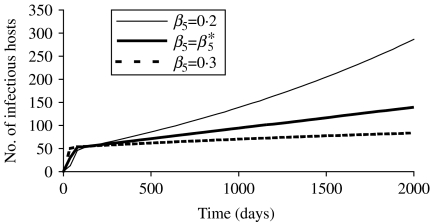
The asymptotic model (M5) looked more like the FD model M2. The conditions for equilibrium are identical. However, in this case the threshold equilibrium value of the transmission coefficient (β₅*=β₂*) represented the value above which all simulations tended to equilibrium. No extinction was observed for upper values of this coefficient. Figure 5 gives an example of simulations with the number of infectious tending clearly to equilibrium or not, and an intermediate simulation obtained with the threshold transmission coefficient. For the considered parameter coefficient in the simulations (cf. Fig. 3), β₅<β₅* and no equilibrium could be obtained.

Fig. 5 — Influence of the value for the transmission coefficient (β₅) on the simulated number of infectious hosts for a model using an asymptotic form of the transmission function (M5). The value β₅* corresponded to the threshold value necessary to reach equilibrium.

We can also determine the classification for the transmission functions as looking like DD or FD depending on the mathematical form of the function (Table 1). In the ‘refuge effect’ (M3) or the negative binomial (M4) models, the transmission functions tended to reach a DD type respectively when h tended to reach 1 or when k was high. On the contrary, the asymptotic form (M5) looked more like the FD type since its denominator term (l+N) was related to a population size term.

DISCUSSION

This paper presents the analysis of the transmission function's effect on a simple epidemiological model. The functions involved in this analysis were chosen on account of their applicability and their biological relevance. The chosen mathematical forms of the transmission function cover a large variety of function types, representing the diversity of host–pathogen systems. Analytical studies on the theoretical approach completed the simulation results and helped in their understanding. Together with the different selected transmission functions, these studies allow us to generalize the results.

The simulated results showed clear differences between the transmission functions, whether the population size was considered constant or increasing. In the former case, the differences concerned the number of susceptible, infectious or recovered hosts when the system reached equilibrium. Simulations with refuge-effect (M3) and negative binomial (M4) models showed lower equilibrium values than those obtained with M1, M2 and M5. In the case of a variable population size, a distinction could be made between functions for which equilibrium was reached (DD M1, M3 and M4), and those which resulted in an exponential population growth (FD M2 and M5). From the simulations with a variable size, the mathematical forms of the horizontal transmission function could be globally divided into either DD or FD types, even though, as shown for instance with frequency-dependence, the occurrence of equilibrium might depend on the chosen parameter values.

From this theoretical model, these results showed evidence of an influence of the transmission function form, whether a DD- or a FD-like form was used. These two forms are both widely used in the literature. Several comparisons have been carried out to find the function that best suits the corresponding host–pathogen system and/or the available data. A theoretical study [20] was dedicated to the comparison between two spatial models, using either a fixed contact area (FCA) or a fixed contact number (FCN) in a cellular automaton, and their corresponding mathematical forms (DD or FD). Both mathematical forms represented equally well FCA or FCN models when the population size was constant, whereas FD best suited both spatial models when this size increased. Comparisons have also been carried out thanks to dedicated experiments [21] dealing with the transmission of pseudorabies virus in pig populations. These authors compared two forms of the transmission functions (βSI and βSI/N) considering the fitting on experimental data. They demonstrated the best-case scenario with the FD form given their data. However, in this experiment, the density of animals was kept constant, as the area occupied increased with the number of animals considered, with two groups of respectively 10 and 40 pigs. This experiment could, therefore, not assess the difference between DD and FD functions [as defined by equations (2) and (4)], which were equivalent in this case. Begon et al. [22] demonstrated that the transmission dynamics of the cowpox virus within two wildlife species was better fitted with a FD than with a DD form. Another comparison of results from an experiment and a model for the study of a moth-virus interaction [23] led to the conclusion that transmission did not follow a DD function. A better adequacy between model results and experimental data was obtained when the transmission function was in the nonlinear form described in equation (5), or with a negative binomial model (M4). The best-case scenario was assessed with a larger determination coefficient r² in the latter cases than with a DD form (respectively 0·97 and 0·96 vs 0·49). However, this best- case scenario was obtained by estimating respectively three and two parameters, whereas only one parameter was needed for a DD function. Increasing the number of parameters to be estimated may also lead to a concomitant increase in the uncertainty associated and to a decrease in the robustness of the model.

A future work could deal with the influence of different transmission functions to a model applied to an actual pathogen spread. Recently, Wonham et al. [24] showed that epidemiological models applied to the spread of West Nile virus were not always using the same transmission function. Three mathematical forms were identified in these host–vector disease models: reservoir or susceptible frequency-dependence, either considering the reservoir or the vector population for the frequency term, and mass action (equivalent to DD). They demonstrated that different values for R₀ could be obtained with these functions, and that it could therefore lead to differing conclusions concerning the control of disease dynamics. However, these authors stated that these different transmission functions applied biologically only at certain population densities, thus justifying their relevance. This kind of study could be carried out for a pathogen that spreads through direct transmission.

In epidemiological models, the relevance of the transmission function used may be assessed on different grounds. First, whenever possible, this function has to correspond to the hypotheses underlying the biological phenomena, even though a direct relation between a mathematical form and host–pathogen interactions is sometimes difficult to establish. Whenever experimental data are available, a statistical fitting is also fruitful for the determination of the transmission function and of the associated parameters. At the very least, a global validation of the model and a sensitivity analysis of the simulated results according to the transmission function and related parameter values should be performed. Even though in the studies quoted in this paper, the comparison between the models and experimental data often showed evidence of a best-case scenario with the FD form, this should not become a general law and all the host–pathogen systems have to be studied specifically.

DECLARATION OF INTEREST

None.

REFERENCES

1.Anderson RM, May RM. Infectious Diseases of Humans. Oxford: Oxford Science Publications; 1992. p. 757. , pp. [Google Scholar]
2.Hurd HS, Kaneene JB. The application of simulation models and systems analysis in epidemiology: a review. Preventive Veterinary Medicine. 1993;15:81–99. [Google Scholar]
3.Valleron AJ. Roles of mathematical modelling in epidemiology [in French] Comptes Rendus de l'Académie des Sciences, Series III: Sciences de la vie. 2000;323:429–433. doi: 10.1016/s0764-4469(00)00153-0. [DOI] [PubMed] [Google Scholar]
4.de Jong MCM. Mathematical modelling in veterinary epidemiology: why model building is important. Preventive Veterinary Medicine. 1995;25:183–193. [Google Scholar]
5.Begon M et al. A clarification of transmission terms in host-microparasite models: numbers, densities and areas. Epidemiology and Infection. 2002;129:147–153. doi: 10.1017/s0950268802007148. [DOI] [PMC free article] [PubMed] [Google Scholar]
6.McCallum H, Barlow N, Hone J. How should pathogen transmission be modelled? Trends in Ecology and Evolution. 2001;16:295–300. doi: 10.1016/s0169-5347(01)02144-9. [DOI] [PubMed] [Google Scholar]
7.Diekmann O et al. The force of infection in populations of varying size: a modelling problem. Journal of Biological Systems. 1995;3:519–529. [Google Scholar]
8.Fromont E, Pontier D, Langlais M. Dynamics of a feline retrovirus (FeLV) in host populations with variable spatial structure. Proceedings of the Royal Society London Series B: Biological Sciences. 1998;265:1097–1104. doi: 10.1098/rspb.1998.0404. [DOI] [PMC free article] [PubMed] [Google Scholar]
9.Hochberg ME. Non-linear transmission rates and the dynamics of infectious disease. Journal of Theoretical Biology. 1991;153:301–321. doi: 10.1016/s0022-5193(05)80572-7. [DOI] [PubMed] [Google Scholar]
10.Hethcote HW, Van Den Driessche P. Some epidemiological models with nonlinear incidence. Journal of Mathematical Biology. 1991;29:271–287. doi: 10.1007/BF00160539. [DOI] [PubMed] [Google Scholar]
11.Barlow ND. A spatially aggregated disease/host model for bovine TB in New Zealand possum populations. Journal of Applied Ecology. 1991;28:777–793. [Google Scholar]
12.Barlow ND. Non-linear transmission and simple models for bovine tuberculosis. Journal of Animal Ecology. 2000;69:703–713. [Google Scholar]
13.Diekmann O, Kretzschmar M. Patterns in the effects of infectious diseases on population growth. Journal of Mathematical Biology. 1991;29:539–570. doi: 10.1007/BF00164051. [DOI] [PubMed] [Google Scholar]
14.Heesterbeek JAP, Metz JAJ. The saturating contact rate in marriage- and epidemic models. Journal of Mathematical Biology. 1993;31:529–539. doi: 10.1007/BF00173891. [DOI] [PubMed] [Google Scholar]
15.Roberts MG. The dynamics of bovine tuberculosis in possum populations, and its eradication or control by culling or vaccination. Journal of Animal Ecology. 1996;65:451–464. [Google Scholar]
16.Anderson RM, May RM. Population biology of infectious diseases: Part 1. Nature. 1979;280:361–367. doi: 10.1038/280361a0. [DOI] [PubMed] [Google Scholar]
17.Briggs CJ, Godfray HCJ. The dynamics of inect-pathogen interactions in stage-structured populations. American Naturalist. 1995;145:855–887. [Google Scholar]
18.Lopez LF et al. Threshold conditions for infection persistence in complex host-vectors interactions. Comptes Rendus Biologie. 2002;325:1073–1084. doi: 10.1016/s1631-0691(02)01534-2. [DOI] [PubMed] [Google Scholar]
19.Coutinho FAB et al. An approximate threshold condition for non-autonomous system: An application to a vector borne infection. Mathematics and Computers in Simulation. 2005;70:149–158. [Google Scholar]
20.Turner J, Begon M, Bowers RG. Modelling pathogen transmission: the interrelationship between local and global approaches. Proceedings of the Royal Society London, Series B: Biological Sciences. 2003;270:105–112. doi: 10.1098/rspb.2002.2213. [DOI] [PMC free article] [PubMed] [Google Scholar]
21.Bouma A, De Jong MCM, Kimman TG. Transmission of pseudorabies virus within pig populations is independent of the size of the population. Preventive Veterinary Medicine. 1995;23:163–172. [Google Scholar]
22.Begon M et al. Transmission dynamics of a zoonotic pathogen within and between wildlife host species. Proceedings of the Royal Society London B: Biological Sciences. 1999;266:1939–1945. doi: 10.1098/rspb.1999.0870. [DOI] [PMC free article] [PubMed] [Google Scholar]
23.Knell RJ, Begon M, Thompson DJ. Transmission of Plodia interpunctella granulosis virus does not conform to the mass action model. Journal of Animal Ecology. 1998;67:592–599. [Google Scholar]
24.Wonham MJ et al. Transmission assumptions generate conflicting predictions in host-vector disease models: a case study in West Nile virus. Ecology Letters. 2006;9:703–725. doi: 10.1111/j.1461-0248.2006.00912.x. [DOI] [PubMed] [Google Scholar]

[ref001] 1.Anderson RM, May RM. Infectious Diseases of Humans. Oxford: Oxford Science Publications; 1992. p. 757. , pp. [Google Scholar]

[ref002] 2.Hurd HS, Kaneene JB. The application of simulation models and systems analysis in epidemiology: a review. Preventive Veterinary Medicine. 1993;15:81–99. [Google Scholar]

[ref003] 3.Valleron AJ. Roles of mathematical modelling in epidemiology [in French] Comptes Rendus de l'Académie des Sciences, Series III: Sciences de la vie. 2000;323:429–433. doi: 10.1016/s0764-4469(00)00153-0. [DOI] [PubMed] [Google Scholar]

[ref004] 4.de Jong MCM. Mathematical modelling in veterinary epidemiology: why model building is important. Preventive Veterinary Medicine. 1995;25:183–193. [Google Scholar]

[ref005] 5.Begon M et al. A clarification of transmission terms in host-microparasite models: numbers, densities and areas. Epidemiology and Infection. 2002;129:147–153. doi: 10.1017/s0950268802007148. [DOI] [PMC free article] [PubMed] [Google Scholar]

[ref006] 6.McCallum H, Barlow N, Hone J. How should pathogen transmission be modelled? Trends in Ecology and Evolution. 2001;16:295–300. doi: 10.1016/s0169-5347(01)02144-9. [DOI] [PubMed] [Google Scholar]

[ref007] 7.Diekmann O et al. The force of infection in populations of varying size: a modelling problem. Journal of Biological Systems. 1995;3:519–529. [Google Scholar]

[ref008] 8.Fromont E, Pontier D, Langlais M. Dynamics of a feline retrovirus (FeLV) in host populations with variable spatial structure. Proceedings of the Royal Society London Series B: Biological Sciences. 1998;265:1097–1104. doi: 10.1098/rspb.1998.0404. [DOI] [PMC free article] [PubMed] [Google Scholar]

[ref009] 9.Hochberg ME. Non-linear transmission rates and the dynamics of infectious disease. Journal of Theoretical Biology. 1991;153:301–321. doi: 10.1016/s0022-5193(05)80572-7. [DOI] [PubMed] [Google Scholar]

[ref010] 10.Hethcote HW, Van Den Driessche P. Some epidemiological models with nonlinear incidence. Journal of Mathematical Biology. 1991;29:271–287. doi: 10.1007/BF00160539. [DOI] [PubMed] [Google Scholar]

[ref011] 11.Barlow ND. A spatially aggregated disease/host model for bovine TB in New Zealand possum populations. Journal of Applied Ecology. 1991;28:777–793. [Google Scholar]

[ref012] 12.Barlow ND. Non-linear transmission and simple models for bovine tuberculosis. Journal of Animal Ecology. 2000;69:703–713. [Google Scholar]

[ref013] 13.Diekmann O, Kretzschmar M. Patterns in the effects of infectious diseases on population growth. Journal of Mathematical Biology. 1991;29:539–570. doi: 10.1007/BF00164051. [DOI] [PubMed] [Google Scholar]

[ref014] 14.Heesterbeek JAP, Metz JAJ. The saturating contact rate in marriage- and epidemic models. Journal of Mathematical Biology. 1993;31:529–539. doi: 10.1007/BF00173891. [DOI] [PubMed] [Google Scholar]

[ref015] 15.Roberts MG. The dynamics of bovine tuberculosis in possum populations, and its eradication or control by culling or vaccination. Journal of Animal Ecology. 1996;65:451–464. [Google Scholar]

[ref016] 16.Anderson RM, May RM. Population biology of infectious diseases: Part 1. Nature. 1979;280:361–367. doi: 10.1038/280361a0. [DOI] [PubMed] [Google Scholar]

[ref017] 17.Briggs CJ, Godfray HCJ. The dynamics of inect-pathogen interactions in stage-structured populations. American Naturalist. 1995;145:855–887. [Google Scholar]

[ref018] 18.Lopez LF et al. Threshold conditions for infection persistence in complex host-vectors interactions. Comptes Rendus Biologie. 2002;325:1073–1084. doi: 10.1016/s1631-0691(02)01534-2. [DOI] [PubMed] [Google Scholar]

[ref019] 19.Coutinho FAB et al. An approximate threshold condition for non-autonomous system: An application to a vector borne infection. Mathematics and Computers in Simulation. 2005;70:149–158. [Google Scholar]

[ref020] 20.Turner J, Begon M, Bowers RG. Modelling pathogen transmission: the interrelationship between local and global approaches. Proceedings of the Royal Society London, Series B: Biological Sciences. 2003;270:105–112. doi: 10.1098/rspb.2002.2213. [DOI] [PMC free article] [PubMed] [Google Scholar]

[ref021] 21.Bouma A, De Jong MCM, Kimman TG. Transmission of pseudorabies virus within pig populations is independent of the size of the population. Preventive Veterinary Medicine. 1995;23:163–172. [Google Scholar]

[ref022] 22.Begon M et al. Transmission dynamics of a zoonotic pathogen within and between wildlife host species. Proceedings of the Royal Society London B: Biological Sciences. 1999;266:1939–1945. doi: 10.1098/rspb.1999.0870. [DOI] [PMC free article] [PubMed] [Google Scholar]

[ref023] 23.Knell RJ, Begon M, Thompson DJ. Transmission of Plodia interpunctella granulosis virus does not conform to the mass action model. Journal of Animal Ecology. 1998;67:592–599. [Google Scholar]

[ref024] 24.Wonham MJ et al. Transmission assumptions generate conflicting predictions in host-vector disease models: a case study in West Nile virus. Ecology Letters. 2006;9:703–725. doi: 10.1111/j.1461-0248.2006.00912.x. [DOI] [PubMed] [Google Scholar]

PERMALINK

Influence of the transmission function on a simulated pathogen spread within a population

T HOCH

C FOURICHON

A-F VIET

H SEEGERS

SUMMARY

INTRODUCTION