SUMMARY
We developed a mathematical model of the transmission dynamics of salmonella to describe an outbreak of S. Cerro infection that occurred in a Pennsylvania dairy herd. The data were collected as part of a cooperative research project between the Regional Dairy Quality Management Alliance and the Agricultural Research Service. After the initial detection of a high prevalence of S. Cerro infection in the herd, a frequent and intensive sampling was conducted and the outbreak was followed for 1 year. The data showed a persistent presence of S. Cerro with a high prevalence of infection in the herd. The dynamics of host and pathogen were modelled using a set of nonlinear differential equations. A more realistically distributed (gamma-distributed) infectious period using multiple stages of infection was considered. The basic reproduction number was calculated and relevance to the intervention strategies is discussed.
INTRODUCTION
Salmonella spp. are frequently isolated from dairy cattle and from various locations within dairy farm environments such as water, feed, manure, and bird droppings. Salmonellosis (the clinical disease caused by Salmonella spp.) can have serious health implications in calves and cattle, but asymptomatic shedding in faeces also occurs [1]. There are more than 2000 known serotypes of S. enterica. The NAHMS Dairy 1996 study showed faecal shedding of Salmonella in 5·4% of cows [2]. The most common serotypes isolated from the faecal samples were Montevideo (21·5%), Cerro (13·3%), Kentucky (8·5%), Menhaden (7·7%), Anatum (6·1%), Meleagridis (6·1%), Muenster (4·7%), and Mbandaka (4·6%). Although the most common salmonellae that cause disease in humans (United States) are S. enterica Typhimurium, Enteritidis, and Heidelberg, all Salmonella are potentially pathogenic.
Presence of Salmonella enterica serotype Cerro (S. Cerro) has been described in several reports from wildlife, food animals, and occasional cases of disease in humans. Specifically, isolations of this serotype have been described from hens' eggs [3], duck eggs [4], captive crocodiles [5], poultry flock and slurry [6, 7], and from asymptomatic dairy and beef cows [8, 9] and bulk tank milk [10]. In humans, S. Cerro was isolated from healthy schoolchildren [11] and occasional cases of disease [12–15]. A European surveillance study reported the endemic presence of S. Cerro in Southern Italy. Human sources (both healthy and diseased), food items, environmental samples and urban sewage plant effluents were positive for this serotype. In this particular environment, S. Cerro prevalence was ranked second only to S. Typhimurium.
Studies from dairy farms such as the one reported by Peek et al. [16] showed the presence of S. Cerro in environmental samples from 1 of 20 herds in Wisconsin. These free stall dairies had no history of clinical salmonellosis. Van Kessel et al. [10] reported in results from 860 dairies from 21 states participating in the 2002 NAHMS study. They observed S. Cerro in the bulk milk of two of these dairies [10].
Modelling of S. Cerro infection patterns within the herd would help to explain the population dynamics and clarify the reason why this organism is able to maintain itself in herds. Modelling of infectious disease in dairy herds has been done before (see e.g. [17, 18]) and often resulted in a better understanding of infection dynamics. Results of these studies were used to design vaccination programmes or to facilitate eradication of the infection from the herd. Salmonella infections have been modelled before [19], using a SIRS model stratified for age and lactation period (dry vs. lactating). The model was used to perform simulations, but was not tested against observed data. In this case study we report the observed endemic presence of S. Cerro on a dairy farm. Our objective is to apply a modified version of the SIR model [20] and the Xiao et al. model [19] to the observed data to study the cause of S. Cerro endemicity of this infection within the herd.
MATERIALS AND METHODS
Farm description
The dairy farm where the samples for this study were collected participates in a multi-state research programme conducted under a cooperative research project between the Regional Dairy Quality Management Alliance (RDQMA) and the Agricultural Research Service (ARS). The farm is located in Pennsylvania and milks ~100 cows. Heifer calves are born on the farm and at ~6 months of age are moved to a contract heifer grower with heifers returning to the farm prior to calving. Participation in the study includes quarterly blood sampling of all lactating animals and bi-annual faecal sampling.
Sampling, sample handling, sample analysis, definition of infection
After the initial detection of salmonella infection on the farm, the faecal sampling frequency was increased and all cows were sampled every 6–8 weeks for ~1 year. Faecal samples were obtained by rectal palpation and placed directly into sterile vials, cooled, and transported overnight to the Environmental Microbial Safety Laboratory of the Agricultural Research Services in Beltsville, Maryland. Upon arrival, ~25 g of faecal material was weighed into a filtered stomacher bag, diluted (2/1) with buffered peptone water (1%) and pummelled in an automatic bag mixer for 2 min. For enrichment of salmonella, 5 ml filtrate was added to 5 ml double-strength tetrathionate broth and incubated at 37°C for 24 h. Enrichment tubes were incubated at 37°C for 24 h and then the broth was streaked (10 μl) onto XLT4 agar (XLT4 agar base with XLT4 supplement, BD Diagnostics, Sparks, MD, USA). Plates were incubated at 37°C and scored at 24 h and 48 h for presumptive salmonella (black colonies). Isolated, presumptive salmonella colonies were transferred from XLT4 plates onto XLT4, Brilliant Green, and L-agar (Lennox Broth base with 1·5% agar; Gibco Laboratories, Long Island, NY, USA). Colonies that exhibited the salmonella phenotype (black on XLT4 and pink on Brilliant Green) were preserved for future analysis. The isolates were stored at −80°C. For some of the isolates, L-agar slants were inoculated and, after incubation at 37°C for 24 h, sent to the National Veterinary Services Laboratories in Ames, IA, USA for serotyping. The serotypes of other isolates were determined with rep-PCR using the ERIC primers as described by Weigel et al. [21]. An isolate with an ERIC-PCR pattern that was similar to a pattern of an isolate serotyped by NVSL was considered that serotype. Not all isolates were serotyped. Culture procedures used in this analysis have an approximate sensitivity of 1 c.f.u./g faeces.
For PCR analysis, biomass from the enrichments was stored at −20°C. The DNA was extracted from these pellets using Mo Bio UltraClean Soil DNA Extraction kits (Mo Bio Laboratories, Inc., Carlsbad, CA, USA) following the manufacturer's directions. The DNA preparations were stored at −20°C and were analysed for the presence or absence of salmonella via real-time PCR at a later date. Real-time PCR was carried out using an adapted conventional PCR method of Rahn et al. [22] and shown by Malorny et al. [23] to detect a wide range of salmonellae. The method was adapted for real-time PCR by the addition of SYBR Green to the assay. Theoretically, this PCR method has an approximate sensitivity of 1 c.f.u./3 g faeces.
For the purpose of this analysis, records of all cows and all samples were combined and displayed longitudinally. We assumed a non-perfect sensitivity and therefore occasional negative faecal culture results were expected even in truly infected animals. For that reason, animals were considered truly longitudinally infected if two of three subsequent samples were faecal-culture positive. An animal was considered negative after a previous infected period when at least two subsequent samples were culture negative. Hence, in some instances the calculated adjusted prevalence of infectious animals was somewhat different from the actual faecal culture-positive prevalence on a specific sampling day. The difference was due to animals that were culture positive before and after this particular sampling day but were negative on this day. To estimate the rate of new infections, the occurrence of a new infection was placed at the midpoint between two sampling days where the first sampling day was negative and the second was culture positive. Each animal contributed days at risk of infection calculated on a daily basis and using the infection assumptions described above.
MODEL FORMULATION
The mathematical model we used was a state-transition model and was adopted from Xiao et al. [19]. As with traditional SIR modelling, the animals in the herd are grouped into three compartments according to their salmonella infection status – those which are susceptible (S), those infected with salmonella and are infectious (I), and those which are recovered from the infection (R). The total number of animals in the herd is given by N=S+I+R. In the present model, we consider that initially all the animals are susceptible to the infection. Once infected, a susceptible individual leaves the susceptible compartment and enters the infectious compartment where it too becomes infectious. The infected animals pass into the recovered compartment unless they exit the herd for other reasons such as death or culling. Because of the high prevalence shortly after the onset of the infection and unusually long persistence of the infection observed in the herd, the latent period is not considered in the model. The loss of immunity is incorporated by allowing animals to pass back into the susceptible compartment from the recovered class. The average rates of entry and exit from each compartment and other relevant parameters calculated from the data, collected from literature, or assumed are summarized in the Table.
Table.
Definition and the parameter estimates for the transition rates and other parameters in the model that describes the transmission dynamics of Salmonella Cerro infection in a dairy herd. The transmission rates are given in units of per month

An important difference in this model from other models describing salmonella dynamics [19, 24] is the consideration of a more realistic distribution of per capita recovery rate, γ. Classical SIR models simply assume an exponential distribution of infectious period, with mean duration of infection equal to 1/γ. While it has been commonly believed that the precise distribution of the infectious period is unimportant, some recent studies show that it has important consequences in the dynamics of infection [25–27] and the model results. In this study, a more realistic distribution of the infectious period, namely a gamma distribution, is included and the model is validated with the actual observed dynamics in the herd. This is especially important when considering the prevalence of infection in a herd-level population as the exponential distribution of infectious period tends to yield unrealistically low prevalence of infection and takes longer [28] for the infection to die out in the herd.
The infectious period distribution can be described in terms of the probability distribution function, p(τ), which gives the survivorship function, P(l), upon integration:
| (1) |
The survivorship function gives the probability for an individual to remain infectious for at least l time units. As opposed to the exponential distribution of the infectious period, a more realistic probability density function, p(τ), of the infectious period can be incorporated in the differential equations. This can be done by the method of multiple stages [27] in which the single infectious compartment of the classical SIR model is replaced by n successive infectious compartments, each with an exponential distribution of the same value of the mean infectious period, 1/γ, with nγ as the rate of progression through the series of the states. Thus the total time spent in the n compartments is just the sum of n exponential distributions. This gives the gamma distribution of the infectious period with the probability density function [27]:
| (2) |
where Γ(n) is the gamma function. The exponential distribution of the infectious period in the classical SIR model is retained when n is set to 1. Since the variance of this distribution is given by 1/(nγ2), it is easy to estimate the number of compartments that should replace the otherwise single infectious compartment so that the variance of the observed distribution of infectious period can be more accurately incorporated in the model.
In order to model the possible indirect transmission due to free-living bacteria in addition to the direct animal-to-animal transmission, we also include the density of the pathogen in the environment. A simplifying assumption was made that all infected individuals shed pathogen into their environment at an equal rate in order to keep the model less complex. Therefore, the density of the bacteria in the environment (W) is simply a function of the number of infected animals shedding the bacteria and the bacterial survival rate in the environment. Here, we make no distinction between local and combined environment [19] and treat W as the total density of the bacteria in the environment.
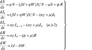
The dynamics of host and pathogen is modeled using a set of nonlinear differential equations which is a modified version of the SIR model. The mathematical equations that incorporate the method of multiple stages [27] in the model are given as:
 |
(3) |
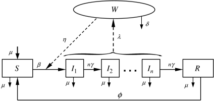
Here, I is the total number of infective animals which is given by the sum of all infective animals in various infectious stages,  . The rates of transition between various compartments and other parameters are defined in the Table and the transmission dynamics described by the above system of nonlinear equations is depicted in Figure 1.
Fig. 1.
Flow diagram representing the transmission dynamics of S. Cerro infection in a dairy herd modelled by the system of equation (3). Parameters are defined in the Table, the compartments are defined as: S is susceptible, Ii is infectious (i=1, … , n), R is immune and W is the environment.
The transition rates were estimated from the adjusted faecal culture data. The distribution of the infectious period was fitted with the gamma distribution in order to calculate the average infectious period, 1/γ, and variance of the distribution, 1/(nγ2), where γ is rate at which an infected individual recovers from the infection. These two quantities give the number of stages that the single infectious compartment needs to be divided in the model described by the set of equations [equation (3)].
The probability that a susceptible animal gets infected depends on the rate of effective contacts with the infected animals. The transmission parameter β(t) was estimated such that the number of new infections at time t+1 is given by the product of the transmission parameter β(t), the number of susceptible animals S(t) and the number of infectious animals I(t) at time t. An animal was considered newly infected if the positive test result was preceded by two consecutive negative test results. In order to estimate the transmission parameter, β, the force of infection for sampling at time t, λ′(t), was estimated as follows:
| (4) |
where Inew(t+1) is the number of new infections in the next sampling and D is the sampling interval which gives the duration of exposure. The parameter β is then calculated as
| (5) |
where N′(t) is the total number of animals at time t in the observed data.
The rate of gain in the number of animals in the herd either due to birth or recruitment of new animals, μ, was expected to be equal to the rate of loss of animals due to death or replacement since the total number of animals in the herd remained approximately constant throughout the study. This rate was estimated from the data and was ~0·03 per month, indicating that animals had an adult herd-life expectation of ~3 years. Because of the high value of β and high prevalence, the rate of loss of immunity was estimated as approximately the inverse of the waiting time until a recovered animal gets re-infected and was 0·22 per month. Other parameters such as the indirect contact rates of infection and the survival of the pathogen in the environment are not known and the parameter values were chosen following the assumption of Xiao et al. [19]. The estimated parameter values are summarized in the Table.
An important concern in epidemiology is whether or not an infectious disease is able to cause an epidemic outbreak. This can be quantified by a single number called the basic reproduction ratio, R0, which measures the effective transmissibility and provides quantitative criteria for disease control. Effective preventive measures of the possible disease outbreaks would be to reduce the value of R0. In deterministic models, the disease-free equilibrium is locally asymptotically stable when R0<1 whereas it is unstable when R0>1 (see for example [29, 30]). This means that the disease dies out if R0<1 and it may maintain itself at an endemic level if R0>1. R0 is given by the product of rate of new infections in an entirely susceptible population and the average duration of infectiousness. As discussed in the Appendix, R0 for the model with n-infectious classes may be obtained by using the next-generation matrix method. The spectral radius of the next-generation matrix, which is the dominant eigenvalue of the same matrix, gives the value of R0. Solving the characteristic equation, we get:
| (6) |
We see that the basic reproduction ratio R0 depends on the number of infectious states which translates into the dependence on the distribution of infectious period. In the case of no indirect transmission, η=0 so that
| (7) |
For a single infectious compartment, this reduces to the well-known expression for R0 as
| (8) |
In order to understand the underlying mechanism of disease transmission, we analysed the model using numerical techniques. The system of differential equations was solved using a fourth-order Runge–Kutta method and the results of disease prevalence and the temporal dynamics were compared with the observed data.
RESULTS
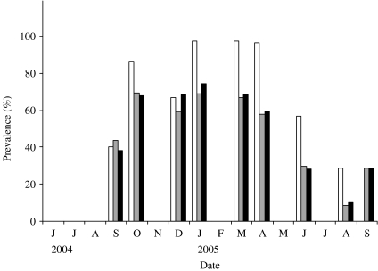
The first faecal sampling of the complete milking herd in March, 2004 indicated that just one (n=102) cow was shedding Salmonella at this time and the isolates from this sample were identified as S. enterica Typhimurium (var. Copenhagen). Six months later, 43·5% of the herd was determined to be infected with Salmonella enterica Cerro (Fig. 2). One animal was shedding S. Kentucky in addition to S. Cerro. In an effort to track the infectious outbreak, the herd was monitored more frequently during the following 12 months. Within 6 weeks the faecal prevalence rate of S. Cerro dramatically increased to 75% and persisted at or near this level for ~6 months. By August, 2005 the number of cows shedding Salmonella had dropped to 9% and the results of a subsequent sampling in September indicated that 29% of the cows were shedding this organism.
Fig. 2.
Prevalence of infection over time. Samples were collected from June 2004 to September 2005. Three prevalence data are shown in this figure: observed prevalence of PCR-positive samples (□), observed faecal culture ( ) and corrected faecal culture (■) (see Materials and methods for an explanation).
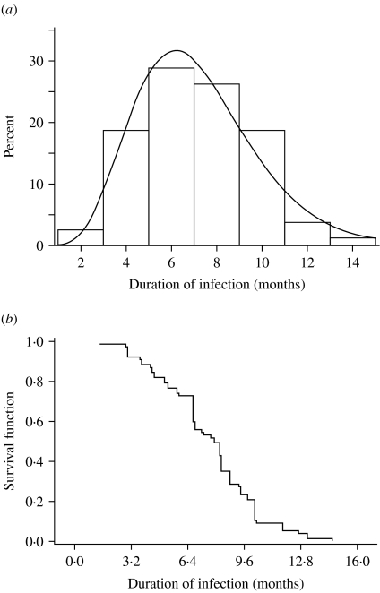
Figure 3a shows the observed distribution of infectious periods from the censored data fitted with a gamma distribution. A plot of the survival probability function of the period of infection is presented in Figure 3b. As shown in these figures, persistent shedding of S. Cerro for unusually long duration was observed in the herd. The average period of infection was found to be 1/γ=7·16 months with the variance=2·5. This gives the number infectious stages as n~128.
Fig. 3.
(a) Distribution of the duration of infection (infectious period). The solid line is the fitted gamma distribution curve. (b) Survival distribution function for the duration of infection.
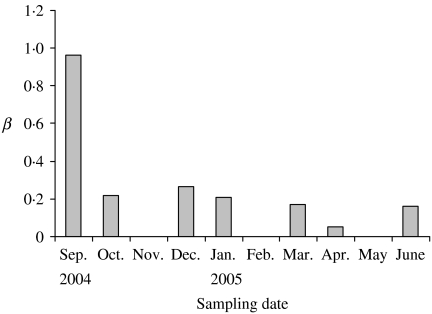
Our results on the estimation of β indicated that its value is high at the onset of infection and it decreases rapidly as the infection reaches to the highest. The estimated value of β for each sampling date is plotted in Figure 4. The figure shows a temporal variation of this transmission parameter. Because the whole herd sampling in March 2004 showed no detection of S. Cerro shedding and the data was collected in regular and smaller intervals only after the first detection of high prevalence of salmonella shedding in September 2004, the numbers of new infections prior to September 2004 sampling were not known and it was not possible to accurately estimate β near the beginning of the outbreak. For simplicity, a constant value of β (=0·9) was chosen that best fit the model results with the observed prevalence. It is straightforward to incorporate the time-dependent β in the model if the data is available.
Fig. 4.
Variation of the transmission parameter β. The value of β is high at the onset of the outbreak and subsequently decreases to a small but relatively constant value.
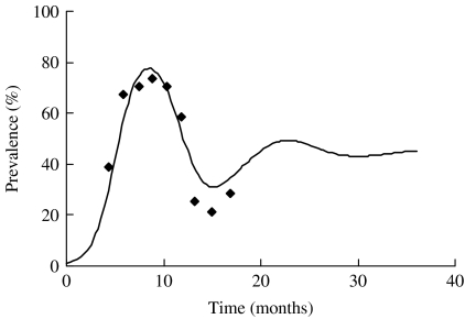
Using the estimated parameters, the simulation was run starting at t=0 when a single infectious individual was introduced in an otherwise totally susceptible population. As expected, the prevalence of infection increased initially with the time and starts to subside once it reaches a maximum. In Figure 5, we plot the simulated prevalence of the infection as a function of time and compare it with the observed prevalence in the herd. For comparison of the simulated infection prevalence with the observed one, the origin of the simulation time t=0 has been shifted so that the peak prevalence of the simulated and observed infection approximately match.
Fig. 5.
Observed (◆) and modelled (—) prevalence of S. Cerro in the herd. The data-points reflect the observed prevalence (adjusted) and the continuous line reflects the modelled prevalence with n=100.
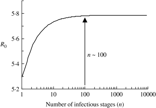
The value of R0 calculated using the average duration of infectiousness and its variance is ~5·8. We plot the dependence of R0 on the number of infectious stages in Figure 6. It is evident from the figure that with the same average duration of infection, exponential distribution of the infectious periods corresponding to n=1 yields a slightly lower estimate of R0. As the distribution becomes sharper with the increase in n, the value of R0 increases as well. R0 asymptotically reaches a constant for a fixed infectious period corresponding to infinitely many infectious stages (n→∞). However, we note that the distribution of the infectious period has little effect on the value of R0 since there is only a small variation in the estimates and R0≫1.
Fig. 6.
The relationship between the number of infectious stages (n) and the basic reproduction ratio (R0).
DISCUSSION
The data that were available for this paper are almost unique. Results of long-term follow-up of a complete milking herd of Salmonella-infected cows has rarely been reported in the literature. In some S. Dublin studies, similar data are available [31], but most of these studies deal with short-term outbreaks often reporting only cross-sectional data [32, 33]. The herd behaviour of S. Cerro that we observed in this case study indicates that this organism is very well adapted to the dairy cow environment. High rates of new infection were combined with a very long duration of infection. Moreover, there were no obvious signs of clinical disease symptoms associated with the infection in cattle. This was not necessarily due to a lack of observation, since small clinical outbreaks of other salmonella infections (S. Typhimurium and S. Kentucky) were previously noted by the herd owner and veterinarian. The data in the current study indicate that this particular infection can maintain itself relatively well in a dairy herd, potentially leading to long-term infectiousness of dairies with this particular strain.
Of particular interest was our observation of the very long duration of infectiousness. The observed mean duration of ~7 months indicates a very long infectious period per shedder. To be able to model this long infectious period with more accurate distribution, an adopted multi-stage model [27] was used. Approximately 100 infectious states were necessary to capture the dynamics of infection.
As with β, other model parameters and rates are likely to have time dependence due to seasonal variation and such seasonal effects may give rise to temporal oscillations in the disease prevalence in the herd. Accurate estimates of the seasonal effects, however, are not readily available and there is a lack of published data in the literature. Here, we aimed at describing the dynamics of the salmonella infection for at least one complete cycle starting from either an infection-free or low prevalence state that matures to a maximum and ultimately the prevalence subsides to a low prevalence. As seen in Figure 5, the model captures the expected dynamics of the S. Cerro infection in the herd. As the actual observed prevalence has an inherent stochastic nature, numbers may not match exactly each month but the qualitative nature of the dynamics is reproduced very well by the model. After the onset of infection, the disease prevalence is high and remains high for a few months. Subsequently, it starts to slide down and hits the lowest observed prevalence in August. The model predicts another smaller peak in the disease prevalence and the height of the second peak may be bigger if we consider time-varying β (decreased to ~0·2 from ~1) so that enough susceptible population is accumulated before hitting a higher force of infection in the next cycle. Continued monitoring of the study herd will permit refinement of the infection dynamics of S. Cerro in subsequent years.
Because of the additional infectious compartments, calculation of R0 was relatively more complex. The eventual estimate of this parameter was ~5·8, indicating that one infectious individual would on average infect 5·8 susceptible animals. This would generally lead to a massive outbreak of infection in a herd where animals freely mingle. The physical layout of this dairy does allow free and more or less random contact between all animals in the herd and we did indeed observe a large outbreak (see Fig. 2).
Although this study reveals the dynamics of infection in only one dairy herd, the data from recent surveys indicate that S. Cerro is able to cause infections in cattle populations [15, 34]. Although this serotype is a relatively rare cause of disease in humans, cases of human disease associated with S. Cerro have been reported in literature [12, 14]. Consequently, prevention or eradication of this infection from cattle herds is desirable. This may not be an easy task, given the high value of R0 that we estimated from the data. Potential control procedures would include additional environmental hygiene practices (i.e. cleaning waterers and feed alleys), separating animals groups (dry cows vs. milking cows) and introducing effective vaccination practices. There is currently very little field data to make a rational prediction with regard to the impact of these practices on the dynamics of infection. More field research is essential to obtain quantitative estimates on the efficacy of these practices.
ACKNOWLEDGEMENTS
Financial support for this work was provided in part by specific cooperative agreements with the United States Department of Agriculture – Agriculture Research Service (USDA-ARS) and the Food Safety Research and Response Networks through a grant from the USDA-CSREES. We also thank the talented staff of the USDA-ARS Environmental Microbial Safety Laboratory for their technical expertise; and R. Ivanek and R. Mitchell for helpful discussions.
APPENDIX
The expression for R0 that also includes the indirect transmission may be obtained using next-generation matrix method. The spectral radius of the next-generation matrix, which is the dominant eigenvalue of the same matrix, gives the value of R0.
From equation (3), we have
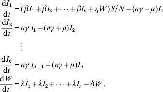 |
For the next-generation matrix, we define the matrices F and V as
where Fi(x) is the number of new infections in the ith compartment from xj infectious individuals and Vi(x) is the net change of animals in the ith compartment by any other means. The rates are evaluated at the disease-free equilibrium x=x0. For the model, these matrices are given as follows:
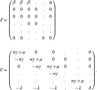 |
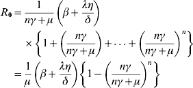
The characteristic equation for the next-generation matrix FV−1 is given by
![\eqalign{\tab \left[ {{1 \over {n\gamma \plus \mu }}\left( {\beta \plus {{\lambda \eta } \over \delta }} \right)\left\{ {1 \plus \left( {{{n\gamma } \over {n\gamma \plus \mu }}} \right)} \right.} \right. \cr \tab\quad \left. {\left. { \plus {\vskip-1.5\ldots} \plus \left( {{{n\gamma } \over {n\gamma \plus \mu }}} \right)^{n} } \right\}} \right]\rmLambda ^{n} \equals 0. \cr}\hfill](https://cdn.ncbi.nlm.nih.gov/pmc/blobs/8553/2870801/b1b8d473666f/S0950268807008400_eqnU5.jpg) |
Solving for the dominant eigenvalue, we get
 |
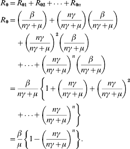
The R0 for the model with n-infectious stages and no indirect transmission may be given by the sum of the contributions from each individual stage
 |
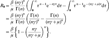
Alternatively, the same expression may be derived from the integral method. Following Lloyd [26], R0 is given by
For gamma-distributed infectious periods, we replace the value of f(τ) from equation (2)
 |
For the single infectious compartment without indirect transmission, the usual expression for R0 is retained
DECLARATION OF INTEREST
None.
REFERENCES
- 1.Warnick LD et al. Risk factors for clinical salmonellosis in Virginia, USA cattle herds. Preventive Veterinary Medicine. 2001;49:259–275. doi: 10.1016/s0167-5877(01)00172-6. [DOI] [PubMed] [Google Scholar]
- 2.Wells SJ et al. Fecal shedding of Salmonella spp. by dairy cows on farm and at cull cow markets. Journal of Food Protection. 2001;64:3–11. doi: 10.4315/0362-028x-64.1.3. [DOI] [PubMed] [Google Scholar]
- 3.Saitanu K et al. Detection of salmonellae in hen eggs in Thailand. Southeast Asian Journal of Tropical Medicine and Public Health. 1994;25:324–327. [PubMed] [Google Scholar]
- 4.Saitanu K, Jerngklinchan J, Koowatananukul C. Incidence of salmonellae in duck eggs in Thailand. Southeast Asian Journal of Tropical Medicine and Public Health. 1994;25:328. [PubMed] [Google Scholar]
- 5.Manolis SC et al. Salmonella in captive crocodiles (Crocodylus johnstoni and C. porosus. Australian Veterinary Journal. 1990;68:102–105. doi: 10.1111/j.1751-0813.1991.tb00764.x. [DOI] [PubMed] [Google Scholar]
- 6.Sunaga Y, Sato S. Detection of salmonella infection in herds by examination of slurry. National Institute of Animal Health Quarterly. 1982;22:39–44. [PubMed] [Google Scholar]
- 7.Riemann H et al. A survey for salmonella by drag swabbing manure piles in California egg ranches. Avian Diseases. 1998;42:67–71. [PubMed] [Google Scholar]
- 8.Dargatz DA et al. Survey of salmonella serotypes shed in feces of beef cows and their antimicrobial susceptibility patterns. Journal of Food Protection. 2000;63:1648–1653. doi: 10.4315/0362-028x-63.12.1648. [DOI] [PubMed] [Google Scholar]
- 9.Beach JC, Murano EA, Acuff GR. Serotyping and antibiotic resistance profiling of salmonella in feedlot and nonfeedlot beef cattle. Journal of Food Protection. 2002;65:1694–1699. doi: 10.4315/0362-028x-65.11.1694. [DOI] [PubMed] [Google Scholar]
- 10.Van Kessel JS et al. Prevalence of salmonellae, listeria monocytogenes, and fecal coliforms in bulk tank milk on US dairies. Journal of Dairy Science. 2004;87:2822–2830. doi: 10.3168/jds.S0022-0302(04)73410-4. [DOI] [PubMed] [Google Scholar]
- 11.Devi S, Murray CJ. Salmonella carriage rate amongst school children – a three year study. Southeast Asian Journal of Tropical Medicine and Public Health. 1991;22:357–361. [PubMed] [Google Scholar]
- 12.Bhore AV, Phadke SA, Joshi BN. Salmonella Cerro causing pyaemia in man – report of a case. Indian Journal of Pathology & Microbiology. 1980;23:309–311. [PubMed] [Google Scholar]
- 13.Le CT. Salmonella vertebral osteomyelitis: a case report with literature review. American Journal of Diseases of Children. 1982;136:722–724. [PubMed] [Google Scholar]
- 14.Fule RP, Kaundinya DV. S. Cerro (18:z4,z23-), a rare serotype isolation from infants with diarrhoea in Ambajogai. Indian Journal of Pathology & Microbiology. 1986;29:205–207. [PubMed] [Google Scholar]
- 15.Mammina C et al. Endemic presence of Salmonella enterica serotype Cerro in southern Italy. Eurosurveillance: European Communicable Disease Bulletin. 2000;5:84–86. doi: 10.2807/esm.05.07.00028-en. [DOI] [PubMed] [Google Scholar]
- 16.Peek SE et al. Isolation of Salmonella spp from the environment of dairies without any history of clinical salmonellosis. Journal of the American Veterinary Medical Association. 2004;225:574–577. doi: 10.2460/javma.2004.225.574. [DOI] [PubMed] [Google Scholar]
- 17.Lam TJ et al. Mathematical modeling to estimate efficacy of postmilking teat disinfection in split-udder trials of dairy cows. Journal of Dairy Science. 1996;79:62–70. doi: 10.3168/jds.S0022-0302(96)76334-8. [DOI] [PubMed] [Google Scholar]
- 18.Hage JJ et al. Transmission of bovine herpesvirus 1 within and between herds on an island with a BHV1 control programme. Epidemiology and Infection. 2003;130:541–552. [PMC free article] [PubMed] [Google Scholar]
- 19.Xiao Y et al. Understanding the dynamics of salmonella infections in dairy herds: a modeling approach. Journal of Theoretical Biology. 2005;233:159–175. doi: 10.1016/j.jtbi.2004.09.015. [DOI] [PubMed] [Google Scholar]
- 20.Anderson RM, May RM. Infectious Diseases of Humans – Dynamics and Control. Oxford: Oxford University Press; 1992. [Google Scholar]
- 21.Weigel RM et al. Comparison of pulsed field gel electrophoresis and repetitive sequence polymerase chain reaction as genotyping methods for detection of genetic diversity and inferring transmission of salmonella. Veterinary Microbiology. 2004;100:205–217. doi: 10.1016/j.vetmic.2004.02.009. [DOI] [PubMed] [Google Scholar]
- 22.Rahn KS et al. Amplification of an invA gene sequence of Salmonella Typhimurium by polymerase chain reaction as a specific method of detection of salmonella. Molecular and Cellular Probes. 1992;6:271–279. doi: 10.1016/0890-8508(92)90002-f. [DOI] [PubMed] [Google Scholar]
- 23.Malorny B et al. Multicenter validation of the analytical accuracy of salmonella PCR: towards an international standard. Applied and Environmental Microbiology. 2003;69:290–296. doi: 10.1128/AEM.69.1.290-296.2003. [DOI] [PMC free article] [PubMed] [Google Scholar]
- 24.Ivanek R et al. A mathematical model for the transmission of Salmonella Typhimurium within a grower-finisher pig herd in Great Britain. Journal of Food Protection. 2004;67:2403–2409. doi: 10.4315/0362-028x-67.11.2403. [DOI] [PubMed] [Google Scholar]
- 25.Mittler JE et al. Influence of delayed viral production on viral dynamics in HIV-1 infected patients. Mathematical Biosciences. 1998;152:143–163. doi: 10.1016/s0025-5564(98)10027-5. [DOI] [PubMed] [Google Scholar]
- 26.Lloyd AL. Destabilization of epidemic models with the inclusion of realistic distributions of infectious periods. Proceedings of the Royal Society of London, Series B: Biological Sciences. 2001;268:985–993. doi: 10.1098/rspb.2001.1599. [DOI] [PMC free article] [PubMed] [Google Scholar]
- 27.Lloyd AL. Realistic distributions of infectious periods in epidemic models: changing patterns of persistence and dynamics. Theoretical Population Biology. 2001;60:59–71. doi: 10.1006/tpbi.2001.1525. [DOI] [PubMed] [Google Scholar]
- 28.Wearing HJ, Rohani P, Keeling MJ. Appropriate models for the management of infectious diseases. PLoS Medicine. 2005;2:0621–0627. doi: 10.1371/journal.pmed.0020174. [DOI] [PMC free article] [PubMed] [Google Scholar]
- 29.Hethcote HW. The mathematics of infectious diseases. SIAM Review. 2000;42:599–653. [Google Scholar]
- 30.Hethcote HW, van den Driessche P. Two SIS epidemiologic models with delays. Journal of Mathematical Biology. 2000;40:3–26. doi: 10.1007/s002850050003. [DOI] [PubMed] [Google Scholar]
- 31.Wray C et al. A three-year study of Salmonella Dublin infection in a closed dairy herd. The Veterinary record. 1989;124:532–537. doi: 10.1136/vr.124.20.532. [DOI] [PubMed] [Google Scholar]
- 32.Trueman KF et al. Salmonella Dublin infection in Queensland dairy cattle. Australian Veterinary Journal. 1996;74:367–369. doi: 10.1111/j.1751-0813.1996.tb15447.x. [DOI] [PubMed] [Google Scholar]
- 33.Wedderkopp A, Stroger U, Lind P. Salmonella Dublin in Danish dairy herds: frequency of change to positive serological status in bulk tank milk ELISA in relation to serostatus of neighbouring farms. Acta Veterinaria Scandinavica. 2001;42:295–301. doi: 10.1186/1751-0147-42-295. [DOI] [PMC free article] [PubMed] [Google Scholar]
- 34.Wells SJ et al. Fecal shedding of Salmonella spp. by dairy cows on farm and at cull cow markets. Journal of Food Protection. 2001;64:3–11. doi: 10.4315/0362-028x-64.1.3. [DOI] [PubMed] [Google Scholar]


