Computational methods for optical molecular imaging

Summary

A new computational technique, the matched interface and boundary (MIB) method, is presented to model the photon propagation in biological tissue for the optical molecular imaging. Optical properties have significant differences in different organs of small animals, resulting in discontinuous coefficients in the diffusion equation model. Complex organ shape of small animal induces singularities of the geometric model as well. The MIB method is designed as a dimension splitting approach to decompose a multidimensional interface problem into one-dimensional ones. The methodology simplifies the topological relation near an interface and is able to handle discontinuous coefficients and complex interfaces with geometric singularities. In the present MIB method, both the interface jump condition and the photon flux jump conditions are rigorously enforced at the interface location by using only the lowest-order jump conditions. This solution near the interface is smoothly extended across the interface so that central finite difference schemes can be employed without the loss of accuracy. A wide range of numerical experiments are carried out to validate the proposed MIB method. The second-order convergence is maintained in all benchmark problems. The fourth-order convergence is also demonstrated for some three-dimensional problems. The robustness of the proposed method over the variable strength of the linear term of the diffusion equation is also examined. The performance of the present approach is compared with that of the standard finite element method. The numerical study indicates that the proposed method is a potentially efficient and robust approach for the optical molecular imaging.

1. Introduction

Being able to study biological features and processes in vivo at the cellular and genetic levels, molecular imaging has embraced as an essential tool for molecular-based drug research and development. It can non-invasively differentiate and quantify normal and diseased conditions and identify variations in disease expression and therapeutic responsiveness for better clinical decision-making. The imaging of gene transcription, signal transduction, and biological pathways allows early diagnosis and individualized therapies, leading to the development of the molecular medicine [1–3]. Molecular imaging has for years fueled innovations and discoveries in biology and medicine. Today, researchers are applying its strengths and wrestling with its challenges in an effort to shed light on molecular secrets deep within living tissues and cells. Among molecular imaging modalities, optical imaging, fluorescent and bioluminescent imaging techniques, in particular, have attracted a remarkable attention for their unique advantages, especially performance and cost-effectiveness. Driving progresses in optical molecular imaging are the development of biocompatible fluorescent and bioluminescent markers, advances in imaging technology, such as temperature-modulated bioluminescent tomography [4], and refinements in the mathematical models. These advances are helping researchers secure the future of optical molecular imaging: improvement of light penetration and detection, image reconstruction and resolution, and disease localization and quantification.

Among various optical molecular imaging techniques [3, 5–8], bioluminescence tomography (BLT) invented by Wang and coworkers in 2002 is an emerging and promising bioluminescent imaging approach [9–12]. The introduction of BLT relative to planar bioluminescent imaging can be, in a substantial sense, compared with the development of X-ray CT based on radiography. Without BLT, bioluminescent imaging is primarily qualitative. However, with BLT, quantitative and localized analysis on a bioluminescent source distribution becomes feasible in a mouse model. BLT is of paramount importance because of the availability of genetically homogeneous inbred strains of mice and the creation of various transgenic strains such as those carrying activated and inducible forms of oncogenes or knockouts of tumor suppressive genes. It is, therefore, part of our endeavor to develop efficient computational algorithms for the reconstruction of BLT. Theoretically, BLT is an inverse source problem involving light propagation through heterogeneous media. Because optical properties are significantly different in different organs of small animal, the physical process is often modeled by a diffusion equation with discontinuous coefficients and singular sources.

The numerical solution of the diffusion equation with discontinuous coefficients and singular sources is a challenging topic in applied mathematics and scientific computing that has attracted much attention in the past decade [13–36]. The discontinuous coefficients induced by heterogeneous media and the possible singular sources lead to the reduction of regularity in the solution. Consequently, ordinary numerical algorithms, such as finite difference methods, finite element methods, and spectral methods, cannot maintain the designed order of convergence and even diverge in the worst scenario. Mathematical treatments of discontinuous coefficients usually involve local modifications of numerical schemes. Therefore, global spectral methods are usually not convenient except for special cases. This class of interface problems have a wide variety of applications to fluid dynamics [37–41], electrodynamics [42–44], material science [20, 45], bioengineering [46], and biomolecular systems [47–49]. Pioneer work in this field was due to Peskin in 1977 [50], who proposed immersed boundary method (IBM) [50–54]. Apart from Peskin's IBM [50–54], a number of other elegant methods have been developed in the literature. Among them, the ghost fluid method proposed by Osher and coworkers [55, 56] is a relatively simple and easy to use sharp interface approach and is often coupled with the level set method. Finite element formulations [46, 57–59] are more suitable for weak solutions. Cai and Deng proposed an upwinding embedded boundary method [60] for dielectric media. Oevermann and Klein proposed a second-order finite-volume-based interface method [61], which uses bilinear ansatz functions on Cartesian grids and compact stencils. A relevant, while quite distinct, approach is the integral equation method for embedding complex geometry [62–64]. A major advance in the field was made by LeVeque and Li [65], who introduced a remarkable second-order sharp interface scheme, the immersed interface method (IIM). Their method has been improved over the past decade [32, 66–69] and widely applied to practical problems.

Owing to the low regularity in the solution and complex geometry, it is very difficult to construct high-order numerical schemes that are particularly desirable for problems involving both heterogeneous media and short waves where conventional local adaptive refinement approaches do not work well. Typical examples are turbulence, combustion, acoustic fluctuation, and high-frequency wave propagation in inhomogeneous media. Cartesian grids are often preferred in these situations because of the bypass of the mesh generation, better temporal stability, and the availability of fast algebraic solvers. Technically, it is possible to construct high-order numerical schemes by properly enforcing interface continuity conditions in the solution and its derivatives [18, 63, 70–72]. In particular, a systematic higher-order method, the matched interface and boundary (MIB) method, was proposed for treating electromagnetic wave propagation and scattering in dielectric media [70]. One unique feature of this approach is that it does not use high-order jump conditions, which require large stencils and are numerically unstable in higher-order schemes. Another feature of the MIB method is that it is a dimension splitting approach, i.e. it splits a multidimensional problem into one-dimensional (1D) ones. It was found that by repeatedly using only the lowest-order jump conditions, an arbitrarily higher-order interface scheme can be constructed in principle [70]. This approach was tested in the fourth-order beam equation with free boundary conditions [73]. Recently, the earlier MIB method has been generalized for solving two-dimensional (2D) elliptic equations with curved interfaces [71, 72]. Simple Cartesian grids, standard finite difference schemes, and lowest-order physical jump conditions are utilized in the MIB method. An important feature of the MIB method is that the physical jump conditions are enforced at each intersecting point of the interface and the mesh lines. In this sense, the MIB method is a sub-grid scheme that is able to overcome the staircase phenomena of the finite difference approximation for complex geometry and delivers arbitrarily higher-order accuracy. Three-dimensional (3D) second-order [49] and 3D high-order MIB schemes [74] have been constructed for complex interfaces.

For practical applications, it is important to deal with elliptic equations with non-smooth interfaces, which are ubiquitous in scientific and engineering, such as wave-guide analysis [75], electromagnetic wave scattering and propagation [76–78], friction modeling [79], plasma-surface interaction [80], and turbulent-flow [81]. In solving differential equations, non-smooth interfaces are referred to as geometric singularities. For a simple two-domain problem, geometric singularities are due to sharp-edged, sharp-wedged, and sharp-tipped interfaces. However, for complex multidomain geometries, the close contact of two smooth domains leads to geometric singularities, which are referred to as contact geometric singularities. This typically happens in mouse models where different organs contact each other. Technically, it is very challenging to construct efficient numerical methods for this class of problems due to the lack of regularity not only in the solution but also in the interface. Commonly used interface methods might not maintain the designed accuracy for this class of problems. Local adaptive approaches [75, 78] exhibit reduced convergence rates and require dramatic mesh refinements in the vicinity of geometric singularities [82]. These approaches fail to work if the solution is highly oscillatory in case of pollution effect [83]. A remarkable result, due to Hou and Liu [19], was only of 0.8th-order convergence obtained with a 2D finite element method formulation for elliptic interface problems with geometric singularities. Recently, we have developed a second-order MIB treatment of sharp-edged and sharp-tipped interfaces in 2D [84] and 3D [74] geometries. The proposed MIB algorithm, particularly with its treatment of singularities, provides the crucial technical foundation to a new generation of Poisson-Boltzmann equation solvers for the electrostatic analysis of biomolecules [48].

The objective of the present work is to explore the utility and usefulness of the MIB method for the diffusion approximation model in optical molecular imaging. In such a technique, the anatomical structures of a small animal and the associated optical properties are normally obtained using a CT/MRI scanner or some alternative methods. Segmentation techniques are used to separate the anatomy of the animal into its major components, such as heart, lungs, liver, stomach, bones, etc. Optical parameters (absorption, reduced scattering), i.e. coefficients of the underpinning optical diffusion equation, are determined by using diffuse reflectance measurements from the biological tissues for various components of the animal. These coefficients may vary continuously over an organ and discontinuously across organs. Although the geometric boundary of each organ is typically smooth, the contact geometric singularities, i.e. singularities caused by the contact of two or more smooth domains, commonly occur. A main task of the present work is to examine the performance of the proposed MIB method for this problem. Another problem of the optical diffusion equation is caused by the amplitude of linear term, which may result in an unstable inversion matrix. This issue is also studied.

The remainder of this paper is organized as follows. In the following section, the theoretical formulation and computational algorithms are given to the optical imaging and the MIB method. Section 3 is devoted to numerical experiments. The proposed MIB method is used to solve the optical diffusion equation, an elliptic equation with various discontinuous coefficients in 2D and 3D settings. Numerical results are compared with those of the finite element analysis, which is a main working horse for our BLT reconstructed at present. This paper ends with a conclusion to summarize the main points.

2. Theoretical Models and Computational Algorithms

2.1. Model of photon propagation

Photon propagation in biological tissue is commonly described by the radiative transfer equation [85, 86]:

$$\theta \cdot \nabla U+{\mu }_{\text{t}}U={\mu }_{\text{s}}{\int }_{S^2}\eta (\theta \theta \text{'})U(x,\theta \text{'})\text{d}\theta +q$$ (1)

where S² is the unit sphere in ℝ³, q is a light source function, U (x, θ) is the radiance in θ∈ S² at x, μ_t = μ_a + μ_s with μ_a and μ_s being absorption and scattering coefficients, respectively, and the scattering kernel η satisfies the normalization condition ∫_S² η(θθ′) dθ′ = 1. Because the radiative transfer equation is a five-dimensional problem, it involves huge computationally cost. With the dominance of scattering over absorption in the optical molecular imaging, the diffusion approximation model is an alternative and provides a quite accurate description of photon propagation [87, 88]:

$$\begin{array}{cc}-\nabla \cdot (\beta \nabla u)+{\mu }_{\text{a}}u=q,& x\in \Omega \\ u(x)+2\beta \frac{\partial u}{\partial n}=g_{\text{in}},& x\in \partial \Omega \end{array}$$ (2)

We also introduce the region boundary Γ as an interface in the numerical problem Γ ⊂ Ω. Here, u = ∫_S²U (x, θ) dθ is the photon fluency rate, g_in is the incoming flux on the boundary ∂Ω, β = 1/[3(μ_a + μ̄_s)], μ̄_s = (1− η̄)μ_s, η̄ = ∫_S² θθ′ η(θθ′)dθ′, and ∂u/∂n denotes the normal derivative at ∂Ω. The source term q could involve singular functions such as Dirac delta functions; in practice, they could be some point light sources with very small supports compared with the computational domain, which would bring discretization difficulties. Owing to the discontinuity of coefficients and singularity of the interface, the regularity of the solution u : Ω → ℝ. is inevitably reduced, especially near the interface. To make the numerical solution unique, the jump conditions are to be prescribed by different practical problems [89]:

$$\begin{array}{cc}[u]=u^{+}-u^{-}=\phi ,& x\in \Gamma \end{array}$$ (3)

$$\begin{array}{cc}[\beta u_n]={\beta }^{+}{u}_n^{+}-{\beta }^{-}{u}_n^{-}=\mathit{\text{ϕ}},& x\in \Gamma \end{array}$$ (4)

where u^± and β^± represent the restrictions of the solutions and coefficients on the edge of each subdomain Ω^±, and $u_n^{\pm }$ denotes limiting values of the normal derivatives along the interface on each side. ϕ and φ are inherent known functions along the interface Γ with necessary smoothness. Reference [89] has proved the existence and uniqueness of this elliptic interface problem. Different organs can have different optical properties; the coefficients β(x) and μ_a are discontinuous across the organs. Thus, the inner domain of Ω is further divided into n subdomains ${\left\{{\Omega }_i\right\}}_{i=1}^n$ by n − 1 interfaces ${\left\{{\Gamma }_i\right\}}_{i=1}^{n-1}$.

2.2. MIB method

In this section, the MIB method is discussed in general ℝ^d dimensional space. Without loss of generality, assume that the computational domain is a compact rectangle [a₁, b₁] × [a₂, b₂] × ⋯ × [a_d, b_d] and uniformly discretized with grid spacing h for simplicity. Then for j ∈ {1, 2, …, d}, N_j = (b_j − a_j)/h is the number of gird points along the x_j direction. Since the MIB is a dimension splitting method for approximating the differential operator ${\sum }_{j=1}^d\partial /\partial x_j(\beta \partial /\partial x_j)$, only the discretization of a specific direction, say x_j*, is illustrated for simplicity. Discretizations of other directions can be easily derived in a similar manner.

Let e₁ = (1, 0, 0, …, 0) and e_j = (0, …, 0, 1, 0, …, 0) be, respectively, the 1st and jth standard coordinate vectors of ℝ^d space and the d-tuple E = (c₁, c₂, …, c_d) be the index of a specific grid point. We denote a non-boundary grid point as X_E (i.e. c_j ∈ {2, 3, …, N_j − 1}), and its function value as u_E = u(X_E). If X_E is near the interface, its discretization scheme depends whether it is a regular point or an irregular point according to the designed convergence order [72]. At a regular point where the discretization scheme does not involve any grid point across the interface, the approximation for the differential operator is the standard central finite difference scheme:

$$\frac{\partial }{\partial x_{j\ast }}\left(\beta \frac{\partial u}{\partial x_{j\ast }}\right)=\frac{{\beta }_{E-(1/2)e_{j\ast }}^{+}}{h^2}{u}_{E-e_{j\ast }}-\frac{{\beta }_{E-(1/2)e_{j\ast }}^{+}+{\beta }_{E+(1/2)e_{j\ast }}^{+}}{h^2}{u}_E+\frac{{\beta }_{E-(1/2)e_{j\ast }}^{+}}{h^2}{u}_{E+e_{j\ast }}+O(h^2)$$ (5)

The MIB scheme at an irregular point where the discretization scheme involves at least one grid point across the interface is described in the following three subsections.

2.2.1. Dimension splitting

The MIB method takes the dimension splitting approach, which reduces a multidimensional interface problem into 1D ones. Therefore, unlike the IIM, the MIB method does not use multidimensional interpolation or multidimensional Taylor expansion. Consequently, the MIB method simplifies the local topological relation near an interface, which is crucial for 3D problems with complex interface geometries. The MIB method provides special schemes around each intersecting point of the given interface and prescribed meshlines. Therefore, at each intersecting point that is not a grid point, there is one meshline, say x_j*, that is a primary direction. In a second-order MIB scheme, if the interface Γ passes between two grid points X_E and X_E+ej*, then X_E and X_E+ej* are a pair of irregular points. Figure 1 gives a 1D projection of the local computational domain and interface in the primary direction, i.e. x_j* direction. For simplicity, we denote the consecutive grid points X_E+kej* (k ∈ {…, −1, 0, 1, …}) on the x_j* axis as i+k and function values u(X_E+kej*) on these grid points as u_i+k.

Figure 1.

Illustration of fictitious values in 1D: dots in solid lines: regular function values and dots in dash lines: fictitious values.

Figure 1 shows how fictitious values f₁ and f₂ are constructed as smoothly extended function values of u⁺ and u⁻ on both sides of the interface along the x_j* direction. The fictitious value f₁ is the extension of the solution in the left domain to the grid point i + 1, and f₂ is the extension of the solution in the right domain to the grid point i, while the vertical line indicates the interface location. Unlike the original function value u that might be discontinuous, both u⁺ (left) and u⁻ (right) are well behaved across the interface. With the assistance of fictitious values, u^± are matched by the jump conditions at the interface by uniform interpolation.

Assume that X₀ ∈ ℝ^d is the position where the interface intersects the mesh line. We discretize the interface jump conditions as follows:

$$[u]=u^{+}-u^{-}=\phi (X_0)$$ (6)

where

$$\begin{array}{l}{u}^{+}=w_{-1}^{+,0}{u}_{i-1}+w_0^{+,0}{u}_i+w_1^{+,0}{f}_1+O(h^3)\\ u^{-}=w_{-1}^{-,0}{f}_2+w_0^{-,0}{u}_{i+1}+w_1^{+,0}{u}_{i+2}+O(h^3)\end{array}$$ (7)

and

$$\begin{array}{c}[\beta u_n]={\beta }^{+}\nabla u^{+}\cdot \text{n}-{\beta }^{-}\nabla u^{-}\cdot \text{n}\\ =\left(\begin{array}{c}{\beta }^{+}{u}_{x_1}^{+}-{\beta }^{-}{u}_{x_1}^{-}\\ {\beta }^{+}{u}_{x_2}^{+}-{\beta }^{-}{u}_{x_2}^{-}\\ ⋮\\ {\beta }^{+}{u}_{x_{j\ast }}^{+}-{\beta }^{-}{u}_{x_{j\ast }}^{-}\\ ⋮\\ {\beta }^{+}{u}_{x_d}^{+}-{\beta }^{-}{u}_{x_d}^{-}\end{array}\right)\cdot n=\phi \text{(}{X}_0\text{)}\end{array}$$ (8)

Here $w_k^{\pm ,l}$ (l ∈ {0, 1}, k ∈ {−1, 0, 1}) are interpolation weights, which can be easily calculated from Reference [90]. The superscripts ± present the two subdomains, and 0, 1 are for the interpolation and the first-order derivative, respectively, and the set of subscripts −1, 0, 1 is the index of grid points.

In jump condition (8), the first derivatives for all directions and from the two domains are all involved due to the $\nabla u^{\pm }={(u_{x_1}^{\pm },u_{x_2}^{\pm },\dots ,u_{x_d}^{\pm })}^{\text{T}}$. Among them, $u_{x_{j\ast }}^{\pm }$ can be easily obtained by interpolation with function values and fictitious values:

$$\begin{array}{l}{u}_{x_{j\ast }}^{+}=w_{-1}^{+,1}{u}_{i-1}+w_0^{+,1}{u}_i+w_1^{+,1}{f}_1+O(h^2)\\ u_{x_{j\ast }}^{-}=w_{-1}^{-,1}{f}_2+w_0^{-,1}{u}_{i+1}+w_1^{+,1}{u}_{i+2}+O(h^2)\end{array}$$ (9)

The evaluation of $u_{x_j}^{\pm }$ by the interpolation formulation for all j = 1, 2, …, d and j ≠ j* is presented in Section 2.2.3.

Symbolically, we assume that $u_{x_j}^{\pm }$ are solved and the fictitious values f₁ and f₂ can totally determined by Equations (6)–(8). Once fictitious values f₁ and f₂ are determined, modified discretizations for ∂/∂x_j*(β∂u⁺/∂x_j*) at grid points u_i and u_i+1 are given as

$$\frac{\partial }{\partial x_{j\ast }}\left({\beta }^{+}\frac{\partial }{\partial x_{j\ast }}{u}^{+}\right)=\frac{{\beta }_{i-1/2}^{+}}{h^2}{u}_{i-1}-\frac{{\beta }_{i-1/2}^{+}+{\beta }_{i+1/2}^{+}}{h^2}{u}_i+\frac{{\beta }_{i+1/2}^{+}}{h_2}{f}_1+O(h)$$ (10)

and

$$\frac{\partial }{\partial x_{j\ast }}\left({\beta }^{-}\frac{\partial }{\partial x_{j\ast }}{u}^{-}\right)=\frac{{\beta }_{i-1/2}^{-}}{h^2}{f}_2-\frac{{\beta }_{i-1/2}^{-}+{\beta }_{i+1/2}^{-}}{h^2}{u}_{i+1}+\frac{{\beta }_{i+1/2}^{-}}{h^2}{u}_{i+2}+O(h)$$ (11)

Methods for the determination of f₁ and f₂ are described in the following two subsections.

Remarks

1. As presented in Figure 1, grid points i − 1 and i are required to be in the same subdomain and so are i + 1 and i + 2. The assumption can always be satisfied by refining the grid mesh for a smooth interface. For sharp-edged interfaces, the grid refinement might not work. A special MIB scheme has been developed to deal with interface singularities in [84].

2. From the discussion above, the second-order MIB scheme can be generalized to higher-order ones (fourth and sixth order) by extending the solution to more fictitious values near the interface. In the MIB method, this is done by repeatedly using lowest-order jump conditions instead of creating higher-order derivatives.

3. In Reference [72], the fictitious values f₁ and f₂ have been shown to be of O(h³), which guarantees the first-order local truncation error and the global second-order convergence of the MIB scheme.

2.2.2. Derivative elimination

In general, at every intersecting point of the interface and mesh lines, there are two original interface conditions and d − 1 additional first-order interface conditions for an elliptic interface in ℝ^d. These d + 1 interface conditions involve 2d first-order derivatives. In the MIB method, we simultaneously determine as fewer fictitious values around an intersecting point as possible so that we have the maximal flexibility in avoiding the determination of many first-order derivatives, which are often difficult to evaluate due to geometric constraints. Nevertheless, we have to determine at least two fictitious values so that both of the original two interface conditions can be implemented at least indirectly. Consequently, we determine only two fictitious values around an intersecting point and, thus, use d − 1 interface conditions to eliminate d − 1 first-order derivatives. The remaining d + 1 derivatives are to be approximated using appropriate grid function values near the intersecting point.

Specifically, jump conditions (3) and (4) are employed to determine two fictitious values f₁ and f₂. Among them, Equation (3) can be easily discretized as in Equation (6). However, the first-order derivatives along all directions on each subdomain are involved in Equation (8).

Two derivatives along the primary direction x_j* can be approximated by Equation (9). For 2d − 2 derivatives along other directions, i.e. $u_{x_j}^{\pm }$ (j = 1, 2, …, d, j ≠ j*), d − 1 interface conditions, which are obtained by differentiating Equation (3) along tangential directions, are used together with Equation (4) to eliminate d − 1 derivatives. There are flexibilities in the selection of d − 1 derivatives from 2d − 2 derivatives. A general principle is to avoid evaluating those derivatives that are difficult to compute due to local geometric constraint and to optimize the resulting matrix of linear algebraic equations. In most cases, we normally evaluate one of $u_{x_j}^{\pm }$, either $u_{x_j}^{+}$ or $u_{x_j}^{-}$.

A closed interface Γ in ℝ^d can be considered as a ℝ^d−1 manifold embedded in a ℝ^d space. Consider a map Φ from ℝ^d−1 to ℝ^d:

$$\Phi :({\stackrel{\sim }{x}}_1,{\stackrel{\sim }{x}}_2,\dots ,{\stackrel{\sim }{x}}_{d-1})\to ({\stackrel{\sim }{x}}_1,{\stackrel{\sim }{x}}_2,\dots ,{\stackrel{\sim }{x}}_{d-1},I({\stackrel{\sim }{x}}_1,{\stackrel{\sim }{x}}_2,\dots ,{\stackrel{\sim }{x}}_{d-1}))$$ 12

where I is a hyperface function. The tangent space of Φ is given as

$$T_{\text{S}}\Phi =\text{span(}{\Phi }_{{\stackrel{\sim }{x}}_1},{\Phi }_{{\stackrel{\sim }{x}}_2},\dots ,{\Phi }_{{\stackrel{\sim }{x}}_{d-1}}\text{)}=\text{span(}{\text{t}}_1,{\text{t}}_2,\dots ,{\text{t}}_{d-1}$$ (13)

where x̃_k (∀k ∈ {1, 2, …, d − 1}) are manifold parameters, and Φ_x̃k are derivatives of Φ with respect to x̃_k. The tangent vectors t_k are not necessarily orthonormal to each other. However, in 2D and 3D practices, these tangent vectors can be orthonormal with appropriate parametrization of the manifold. From Equation (6), the gradient jump at the interface can be decomposed into d − 1 tangential jump conditions:

$$[\nabla u]\cdot {\text{t}}_j=\underset{h\to 0}{{\displaystyle lim}}\frac{\phi (x+h{\mathbf{\text{t}}}_j)-\phi (x)}{h}={\phi }_{{\mathbf{\text{t}}}_j},j=1,2,\dots ,d-1$$ (14)

With the jump condition (4), a d × 2d system results in

$$(P^{+},-P^{-})\left(\begin{array}{c}\nabla u^{+}\\ \nabla u^{-}\end{array}\right)=\left(\begin{array}{c}{\phi }_{{\text{t}}_1}\\ {\phi }_{{\text{t}}_2}\\ ⋮\\ {\phi }_{{\text{t}}_{d-1}}\\ \phi \end{array}\right)$$ (15)

where

$$P^{+}=\left(\begin{array}{c}{\mathbf{\text{t}}}_1^{\text{T}}\\ {\mathbf{\text{t}}}_2^{\text{T}}\\ ⋮\\ {\mathbf{\text{t}}}_{d-1}^{\text{T}}\\ {\beta }^{+}{\mathbf{\text{n}}}^{\text{T}}\end{array}\right),P^{-}=\left(\begin{array}{c}{\mathbf{\text{t}}}_1^{\text{T}}\\ {\mathbf{\text{t}}}_2^{\text{T}}\\ ⋮\\ {\mathbf{\text{t}}}_{d-1}^{\text{T}}\\ {\beta }^{-}{\mathbf{\text{n}}}^{\text{T}}\end{array}\right)$$ (16)

In Equation (15), only one of each remaining $u_{x_j}^{\pm }$ is to be approximated. Therefore, d − 1 variables need to be eliminated and it is always possible to eliminate d − 1 variables from d-independent equations. Since the tangent vectors and the normal vector are linearly independent, there is a well-defined equation after the elimination. Without loss of generality, assume that $u_{x_j}^{+}$ is to be eliminated from the system and the equation left from the elimination is

$$c_1{u}_{x_{j\ast }}^{+}+c_2{u}_{x_{j\ast }}^{-}+\sum _{j=3,j\ne j\ast }^d{c}_j{u}_{x_j}^{-}=\sum _{j=1}^{d-1}{\stackrel{\sim }{c}}_j{\phi }_{{\mathbf{\text{t}}}_j}+{\stackrel{\sim }{c}}_d\mathit{\text{ϕ}}$$ (17)

where c_j and c̃_j are coefficients after the elimination. Finally, Equations (6) and (17) are used to determine the two fictitious values f₁ and f₂.

2.2.3. Derivative evaluation

After the elimination of d − 1 derivatives, we have to evaluate d − 1 derivatives. This is a difficult task for complex interfaces and is a challenging task for interfaces with geometric singularities. The evaluations are pursued along x_j (j = 1, 2, …, d, j ≠ j^*) direction but in general not along any x_j axis. In 2D, the evaluation must compute in the x_j*− x_j plane. In higher dimensions, the evaluation can be pursued with more flexibilities. In general, we evaluate a derivative in a specific x_j − x_i plane so that the resulting matrix is relatively diagonal and symmetric with respect to the given geometric constraint. Let us assume that x_j* − x_j be such a choice and denote the consecutive grid points X_E+mej*+nej along the x_j* axis and x_j axis as (i+m, j+n), and the function values u(X_E+mej*+nej) as u_i+m,j+n, where m, n∈{…, −2, −1, 0, 1, 2, …}; see Figure 2. Figures 2(a) and (b) illustrate situations where irregular points are off the interface and right on the interface, respectively. The curve is the local geometry of the interface, dots are grid points, and red ones are the pair of irregular points corresponding to the target point (i, j) where the fictitious values locate.

Figure 2.

(a) Off interface irregular point and (b) on interface irregular point.

When the irregular points are off the interface, three auxiliary function values u_o,E, u_o,1, and u_o,2 along the auxiliary line x_j* = x_o are needed to approximate $u_{x_j}^{-}$, where x_o is the j* component of X_o. Hence, $u_{x_j}^{-}$ is approximated by the first-order derivative scheme:

$$u_{x_j}^{-}=p_1{u}_{o,E}+p_2{u}_{o,1}+p_3{u}_{o,2}$$ (18)

where p₁, p₂, and p₃ are derivative weights.

Unfortunately, u_o,E, u_o,1, and u_o,2 are not available since they do not locate on any grid point. Therefore, they are to be obtained from function values on other nearby grid points on the corresponding mesh lines.

The auxiliary value u_o,E locates between the irregular points (i, j) and (i + 1, j), which can be obtained with fictitious values:

$$u_{0,E}=(w_{-1}^{-,0},w_0^{-,0},w_1^{-,0})\cdot {(f_2,u_{i+1,j},u_{i+2,j})}^{\text{T}}$$ (19)

However, the auxiliary values u_o,1 and u_o,2 have to be interpolated by other nearby values:

$$\begin{array}{l}{u}_{o,1}=({\stackrel{\sim }{w}}_{-1}^{-,0},{\stackrel{\sim }{w}}_0^{-,0},{\stackrel{\sim }{w}}_1^{-,0})\cdot {(u_{i+1,j+1},u_{i+2,j+1},u_{i+3,j+1})}^{\text{T}}\\ u_{o,2}=({\overline{w}}_{-1}^{-,0},{\overline{w}}_0^{-,0},{\overline{w}}_1^{-,0})\cdot {(u_{i,j+2},u_{i+1,j+2},u_{i+2,j+2})}^{\text{T}}\end{array}$$ (20)

Note that all the grid points used in interpolating the auxiliary points have to be in the same subdomain. For the example showed in Figure 2(a), by the assumption that after eliminating the $u_{x_j}^{+}$ and approximating $u_{x_j}^{-}$, all the gird points used to interpolate u_o,1 and u_o,2 should be in the Ω⁻ domain (there is no restriction for u_o,E since fictitious values are involved). Therefore, the grid points (i, j + 2), (i + 1, j + 2), and (i + 2, j + 2) are the closest grid points to interpolate u_o,2. However, for u_o,1, the gird point (i, j + 1) is in the Ω⁺ domain, and the closest grid points for u_o,1 are (i + 1, j + 1), (i + 2, j + 1), and (i + 3, j + 1). Therefore, the final expression for $u_{x_j}^{-}$ is

$$\begin{array}{l}{u}_{x_j}^{-}=[p_1,p_2,p_3]\cdot \left[\begin{array}{ccccccccc}{w}_{-1}^{-,0}& w_0^{-,0}& w_1^{-,0}& 0& 0& 0& 0& 0& 0\\ 0& 0& 0& {\stackrel{\sim }{w}}_{-1}^{-,0}& {\stackrel{\sim }{w}}_0^{-,0}& {\stackrel{\sim }{w}}_1^{-,0}& 0& 0& 0\\ 0& 0& 0& 0& 0& 0& {\overline{w}}_{-1}^{-,0}& {\overline{w}}_0^{-,0}& {\overline{w}}_1^{-,0}\end{array}\right]\\ \times [f_2,u_{i+1,j},u_{i+2,j},u_{i+1,j+1},u_{i+2,j+1},u_{i+3,j+1},u_{i,j+2},u_{i+1,j+2},u_{i+2,j+2}]\end{array}$$

From the above equation, we can see that $u_{x_j}^{-}$ is actually a linear combination of some unknown function values on grid points around the irregular point u_i,j. By repeating the same procedure to other coupled x_j*−x_j planes, all similarly structured $u_{x_j}^{-}$ can be determined. Together with jump condition (17), two unknown fictitious values f₁ and f₂ can be determined.

If the target irregular point is right on the interface, as showed in Figure 2(b), the calculation of fictitious values is similar.

At the end of this paper, applications of the MIB scheme are given. The 2D MIB scheme is useful to interface problems in plastic membrane, electromagnetic wave propagation, etc. When d = 2, the following normal vector and tangential vector are usually implemented as

$$\begin{array}{c}\mathbf{\text{n}}=\text{(cos}\theta ,\text{sin}\theta \text{)}\\ \mathbf{\text{t}}=\text{(}-\text{sin}\theta ,\text{cos}\theta \text{)}\\ p^{\pm }=\left(\begin{array}{cc}-sin\theta & cos\theta \\ {\beta }^{\pm }cos\theta & {\beta }^{\pm }sin\theta \end{array}\right)\end{array}$$ (21)

where θ is the angle between the positive direction of the x-axis and the normal vector of the interface. It is easy to show that n and t are orthonormal.

For the MIB scheme used in the implicit solvent model for electrostatics analysis in molecular biology or in biomedical image computation, we consider a 3D MIB scheme. The normal vector and tangential vectors can be chosen as

$$\begin{array}{l}\mathbf{\text{n}}=(sin\psi cos\theta ,sin\psi sin\theta ,cos\psi )\\ {\mathbf{\text{t}}}_1=(-cos\psi cos\theta ,-cos\psi sin\theta ,sin\psi )\\ {\mathbf{\text{t}}}_2=(-sin\theta ,cos\theta ,0)\\ p^{\pm }=\left(\begin{array}{ccc}-cos\psi cos\theta & -cos\psi sin\theta & sin\psi \\ -sin\theta & cos\theta & 0\\ {\beta }^{\pm }sin\psi cos\theta & {\beta }^{\pm }sin\psi sin\theta & {\beta }^{\pm }cos\psi \end{array}\right)\end{array}$$ (22)

where θ and ψ are the azimuth and zenith angles with respect to the normal direction. The explicit expressions of the fictitious values are referred to References [71, 84].

3. Numerical Results and Discussions

In this section, the performance of the MIB scheme for solving the optical diffusion equation (2) is examined in 2D and 3D cases with various interfaces. The results of the finite element method (FEM) are also presented for a comparison in many cases with smooth interfaces. The FEM discretizes the solution u(x) directly and handles complex computational domains very well since the discretization of the computational domain does not have to be uniform. The second-order convergence of the FEM used for elliptic interface problems in 2D cases is proved in [89].

The solutions are prescribed as continuous but non-differentiable along the interfaces in Case 1, Case 2, and Case 6 in order to compare the accuracy and convergence of the FEM and the MIB. In Case 3, Case 4, and Case 5, interfaces are considerably more complex with geometric singularities. For these problems, it is difficult to design analytical solutions that are continuous across the interface. Although the present FEM does not handle problems with discontinuous solutions, the MIB method is robust for problems with discontinuous solutions. Meanwhile, large contrast in diffusion coefficients across the interface is also studied. In Case 6, 3D interfaces are considered to examine the proposed MIB and to compare with the FEM. In Case 7, a mouse model is employed to explore the feasibility of the MIB scheme in BLT analysis. The strength of the linear term is varied to examine the robustness of the proposed MIB method.

3.1. 2D cases

Through this subsection, the computational domains are defined as the square [−1, 1] × [−1, 1] for simplicity. The error between the numerical solution and the analytic solution is measured in the L_∞ norm.

Case 1

The computational domains are defined as the square [−1, 1] × [−1, 1] including a circular $\sqrt{x^2+y^2}\le \frac{1}{2}$ as the interface. The diffusion coefficient is

$$\beta =\{\begin{array}{ll}2,& r=\sqrt{x^2+y^2}\le 0.5\\ 10,& r>0.5\end{array}$$ (23)

the absorption coefficient is

$${\mu }_{\text{a}}=\{\begin{array}{ll}0.01,& r=\sqrt{x^2+y^2}\le 0.5\\ 0,& r>0.5\end{array}$$ (24)

and the source term is

$$q(x,y)=\{\begin{array}{ll}-8.0+0.01r^2,& r=\sqrt{x^2+y^2}\le 0.5\\ -8(x^2+y^2)-4.0,& r>0.5\end{array}$$ (25)

The analytic solution is given by

$$u(x,y)=\{\begin{array}{ll}{r}^2,& r=\sqrt{x^2+y^2}\le 0.5\\ \frac{r^4}{20}+\frac{r^2}{10}+\frac{71}{320},& r>0.5\end{array}$$ (26)

Figure 3 provides the plot of numerical solution (left) and the L_∞ error from the MIB scheme (right). It is seen from the graph that the solution is continuous with moderately sharp jump in the directives.

Figure 3.

Numerical solution (a) and L_∞ error (b) for Case 1.

The jump conditions are [u] = 0 and [βu_n] = 0.75. Table I presents the numerical solutions from the second-order MIB scheme and the FEM. In this case, since the interface is relatively simple, the MIB method achieves its second-order convergence as expected. Owing to the non-uniform mesh, the accuracy of the FEM is similar to that of the MIB under a comparable coarse mesh and gets better at finer meshes. Its convergence is approximately third-order.

Table I.

Errors of numerical solutions from the MIB and the FEM for Case 1.

	Second-order MIB			FEM
nx × ny	L∞ norm	Order	Nxy	L∞ norm	Order
20 × 20	2.144 (−4)		408	1.838 (−4)
40 × 40	5.129 (−5)	2.1	1632	2.445 (−5)	2.9
80 × 80	1.516 (−5)	2.2	6528	3.105 (−6)	2.9
160 × 160	3.603 (−6)	2.1	26112	3.754 (−7)	3

Case 2

In this case, we consider a relatively complicated computational domain described by polar equation $r_0=\frac{1}{2}(1+asin2\theta )$. Here θ is the polar angle. The FEM is robust for a non-rectangular computational domain. For the MIB scheme, we immerse the irregular domain into a larger rectangle, then convert the problem into an interface one. The boundary of original domain is treated as an interface with the prescribed boundary condition.

In the governing equation, the diffusion coefficients are

$$\beta =\{\begin{array}{ll}1,& r\le \frac{1}{2}(1+asin2\theta )\\ 10& \text{otherwise}\end{array}$$ (27)

and absorption coefficients

$${\mu }_{\text{a}}=\{\begin{array}{ll}0.05,& r\le \frac{1}{2}(1+asin2\theta )\\ 0& \text{otherwise}\end{array}$$ (28)

The exact solution is

$$u(x,y)=\{\begin{array}{ll}{(x+y)}^4-4{(x^2+y^2)}^3,& r=\sqrt{x^2+y^2}\le \frac{1}{2}(1+asin2\theta )\\ 0& \text{otherwise}\end{array}$$ (29)

The source term q can be derived accordingly. We set the parameter a = 1, then u is still continuous but not differentiable at the interface. There are two cusps at the origin, see Figure 4(a), which could lead to computational difficulties in a uniform discretization. However, since the solution decays near the cusps, this problem is not challenging. The comparison of numerical solutions from the FEM and the MIB is given in Table II.

Figure 4.

Computational domain (a) and numerical solution (b) for Case 2.

Table II.

Errors of numerical solutions from the MIB and the FEM for Case 2.

	Second-order MIB			FEM
nx × ny	L∞ norm	Order	Nxy	L∞ norm	Order
40 × 40	1.114 (−2)		1444	2.900 (−3)
80 × 80	2.661 (−3)	2.1	4874	6.514 (−4)	2.5
160 × 160	4.475 (−4)	2.5	28576	5.679 (−5)	2.7

Figure 4(b) indicates that the solution has a relatively sharp jump along the normal direction of the interface. From Table II, it can be seen that the MIB scheme maintains its second-order convergence. The FEM shows more flavored accuracy due to its ability of dealing with complex computational domains.

Case 3

The interface is designed as a cardioid whose equation in the polar coordinate is given by r₀ = a (1 − cos θ). Figure 5 presents the geometry. We have set the computational domain very close to the geometric boundary to indicate that the proposed MIB method is not sensitive to the setting.

Figure 5.

Computational domain (a) and numerical solution (b) for Case 3.

The source term is

$$q(x,y)=\{\begin{array}{ll}0.003(x^2+y^2)-16.8,& r=\sqrt{x^2+y^2}\le a(1-cos\theta )\\ 2.2k^{2}sin(k(x+y))& \text{otherwise}\end{array}$$ (30)

with diffusion coefficients

$$\beta =\{\begin{array}{ll}0.42,& r=\le a(1-cos\theta )\\ 1.1& \text{otherwise}\end{array}$$ (31)

and absorption coefficients

$${\mu }_{\text{a}}=\{\begin{array}{ll}0.0003,& r\le a(1-cos\theta )\\ 0& \text{otherwise}\end{array}$$ (32)

The solution is discontinuous at the interface and is given by

$$u(x,y)=\{\begin{array}{ll}10(x^2+y^2),& r=\sqrt{x^2+y^2}\le a(1-cos\theta )\\ sin(k(x+y))& \text{otherwise}\end{array}$$ (33)

It is seen from Figure 5(a) that there is a sharp corner at the origin, which leads to difficulties in the computation. The present FEM does not apply to this problem due to the discontinuity of the solution.

We set parameters a = 0.5 and k = 4. Figure 5(b) indicates that the solution has relatively sharp jumps both in u and βu_n, and the numerical error and convergence order are provided in Table III. The designed second-order convergence is obtained.

Table III.

Errors of numerical solutions for Case 3 and Case 4.

	MIB for Case 3			MIB for Case 4
nx × ny	L∞ norm	Order	nx × ny	L∞ norm	Order
20 × 20	1.623 (−1)
40 × 40	3.285 (−2)	2.3	25 × 25	5.017 (−3)
80 × 80	8.515 (−3)	1.9	50 × 50	1.333 (−4)	1.9
160 × 160	2.051 (−4)	2.0	100 × 100	4.944 (−5)	1.6

Case 4

In this case the interface is designed to be $r_0=\frac{1}{2}cos\theta ({sin}^2\theta -\frac{2}{5})$. The solution is designed as

$$u(x,y)=\{\begin{array}{ll}2+xy,& r=\sqrt{x^2+y^2}\le \frac{1}{2}cos\theta ({sin}^2\theta -0.4)\\ sin(kx)\ast sin(ky)/10& \text{otherwise}\end{array}$$ (34)

The piecewise continuous diffusion coefficients are given as

$$\beta =\{\begin{array}{ll}{x}^2+y^2,& r=\le \frac{1}{2}cos\theta ({sin}^2\theta -0.4)\\ 1& \text{otherwise}\end{array}$$ (35)

The absorption coefficients are set to

$${\mu }_{\text{a}}=\{\begin{array}{ll}0.12,& r=\le \frac{1}{2}cos\theta ({sin}^2\theta -0.4)\\ 0& \text{otherwise}\end{array}$$ (36)

The parameter k is set to k = 4 and the source term q can be derived accordingly.

Figure 6 shows the computational domain and numerical solution. The comparison with the exact solution is provided in Table III. From the performance of the MIB for variable β and large contrasting β, it can be concluded that the MIB scheme is not sensitive to the variations in the diffusion coefficients.

Figure 6.

Computational domain (a) and numerical solution (b) for Case 4.

Case 5

In the last 2D example, an interesting six-petal-flower-like interface is employed. It can be easily described by a polar equation $r_0=\frac{1}{2}(1+\frac{1}{2}sin6\theta )$.

The analytic solution is given by

$$u(x,y)=\{\begin{array}{ll}\frac{1}{4}+sin(x)sin(y),& r=\sqrt{x^2+y^2}\le \frac{1}{2}[1+\frac{1}{2}sin6\theta ]\\ (x^2+y^2)/5& \text{otherwise}\end{array}$$ (37)

with diffusion coefficients

$$\beta =\{\begin{array}{ll}0.17& r\le \frac{1}{2}[1+\frac{1}{2}sin(6\theta )]\\ 0.55& \text{otherwise}\end{array}$$ (38)

and absorption coefficients

$${\mu }_{\text{a}}=\{\begin{array}{ll}0.1,& r\le \frac{1}{2}[1+\frac{1}{2}sin(6\theta )]\\ 0.01& \text{otherwise}\end{array}$$ (39)

The source term q can be easily derived.

Figure 7 indicates sharp jump conditions. The MIB scheme works well when solutions present totally different behaviors in two subdomains. The accuracy and convergence are very similar to those in previous examples and are not listed. The computational domain and numerical solution are presented in Figure 7.

Figure 7.

Computational domain (a) and numerical solution (b) for Case 5.

3.2. 3D cases

For applications in biomedical imaging, it is necessary to examine the proposed MIB scheme in 3D cases for numerical accuracy, rate of convergence, and CPU time. In this section, we provide the results of the MIB scheme and the FEM for 3D cases. First, we use a simple spherical interface and an ellipsoid interface, which is a good representative for smooth surfaces so that higher-order MIB schemes can be applied. Following these tests we employ a mouse model to illustrate applications in biomedical imaging. The kidney and heart embedded in mouse's body are good examples of interface problems. Actually, it is a multi-domain problem since the material coefficients in two organs can be different.

Case 6(a)

Consider a 3D version of Case 1. The 3D optical diffusion equation in the cube domain [−1, 1] × [−1, 1] × [−1, 1] with a spherical interface $r_0=\sqrt{x^2+y^2+z^2}=0.5$. This is a case where one can easily design a continuous solution across the interface so that the FEM can be applied and compared. The source term is

$$q(x,y)=\{\begin{array}{ll}0.01r^2-8.0,\hfill & r=\sqrt{x^2+y^2+z^2}\le 0.5\hfill \\ -10(x^2+y^2+z^2)-6.0,\hfill & r>0.5\hfill \end{array}$$ (40)

The analytic solution is given by

$$u(x,y)=\{\begin{array}{ll}{r}^2,\hfill & r=\sqrt{x^2+y^2+z^2}\le 0.5\hfill \\ \frac{r^4}{20}+\frac{r^2}{10}+\frac{71}{320},\hfill & r>0.5\hfill \end{array}$$ (41)

The coefficients are the same as those in Case 1, while in a 3D form. Under these assumptions, jump conditions are still [u] = 0 and [βu_n] = 0.75.

Table IV presents the numerical results obtained from the MIB scheme. It is seen that the MIB maintains its second-order convergence when the grid points increase and its accuracy holds as well as it does for the 2D problem. Results of high-order MIB schemes are omitted for this problem. Table V presents the results generated from the FEM. For 3D computation, our computer cannot afford too dense mesh grids for the FEM due to limited memory. Therefore, only a few computational results for the FEM under affordable mesh sizes are provided. The FEM for this case shows good accuracy in comparison with the MIB scheme at a very coarse mesh. However, as discussed in [66], the FEM errors usually do not decrease monotonously for interface problems. This phenomenon of the convergence oscillation is reflected in Tables V and VII. In contrast, the MIB scheme demonstrates a consistent pattern of convergence.

Table IV.

Errors of numerical solutions from the MIB for Case 6(a).

nx × ny	L∞ norm	Order	CPU
20 × 20 × 20	3.900 (−4)		0.34
40 × 40 × 40	7.970 (−5)	2.3	6.9
80 × 80 × 80	1.968 (−5)	2.0	113

Table V.

Errors of the FEM results for Case 6(a).

Element number	803	3035	9877	18 723	32 040	33 603
Error	9.90 (−3)	3.50 (−3)	6.70 (−3)	1.00 (−3)	6.80 (−3)	2.00 (−3)
CPU time	0.3	0.8	4.9	15.6	219	235
Order		2.3	−1.6	8.9	−11	77

Table VII.

Errors of the FEM results for Case 6(b).

Element number	3944	7172	15 136	18 534	23 218	36 221
Error	8.297 (−1)	8.370 (−1)	8.535 (−1)	4.220 (−1)	4.584 (−1)	3.861 (−1)
CPU time	1.65	4.48	27.23	36.4	61.26	117.54
Order		−0.01	−0.02	1.2	−1.2	0.22

Case 6(b)

Consider the 3D optical diffusion equation on the computational domain [−5, 5] × [−5, 5] × [−5, 5] and the interface is given as an ellipsoid:

$$\frac{x^2}{9}+\frac{y^2}{4}+\frac{z^2}{4}=1$$ (42)

The solution is designed as

$$u(x,y)=\{\begin{array}{ll}4x^2+9y^2+9z^2-36\hfill & \text{inside}\hfill \\ sin((4x^2+9y^2+9z^2-36)/20)\hfill & \text{otherwise}\hfill \end{array}$$ (43)

with diffusion coefficients

$$\beta =\{\begin{array}{ll}0.1& \text{inside}\\ 8& \text{otherwise}\end{array}$$ (44)

and absorption coefficients

$${\mu }_{\text{a}}=\{\begin{array}{ll}0.15& \text{inside}\\ 0& \text{otherwise}\end{array}$$ (45)

Table VI presents the second- and fourth-order MIB scheme. From the table we can see that the designed convergence orders are realized. This is especially valuable for 3D problems. When the computational domain is large, a high-order scheme offers the required accuracy at a relatively coarse mesh.

Table VI.

Errors of second- and fourth-order MIB for 3D computation in Case 6(b).

	Second-order MIB				Fourth-order MIB
nx × ny × nz	L∞ norm	Order	CPU	nx × ny × nz	L∞ norm	Order	CPU
20 × 20 × 20	7.525 (−1)		0.5	25 × 25 × 25	5.160 (−1)		2.7
40 × 40 × 40	1.493 (−1)	2.3	6.7	50 × 50 × 50	1.102 (−2)	5.5	33.9
80 × 80 × 80	3.596 (−2)	2.0	131	100 × 100 × 100	4.452 (−4)	4.6	452

Owing to limited computer memory, we can only evaluate this model with the FEM at most with 36 221 elements. Table VII lists the numerical error, convergence order and CPU time for the FEM. It is seen that the FEM has a good accuracy at a coarse mesh. However, it fails to show convergence as the mesh is refined. The FEM also costs more CPU time than the MIB does. The performance of the FEM depends heavily on the mesh quality. It is possible to obtain better the FEM results by mesh optimization. However, because the possible presence of interface singularities, such as cusps, sharp-edge wedges and sharp tips, it is difficult for the FEM to demonstrate second-order convergence. To our knowledge, the best FEM results in the literature were of 0.8th-order convergence obtained by Hou and Liu [19], for 2D interface problems with geometric singularities.

Case 7(a)

As the last test we employ a real mouse geometric model to explore the utility of the proposed MIB for the analysis of biomedical imaging, as shown in Figure 8. For convenience, the mouse model is embedded in a rectangle domain with dimensions [−108, 113] × [−35, 53] × [−33, 33]. The mouse model itself has two domains, the muscle parts (denoted as Ω₂ region) and organ parts (heart and kidney, denoted as Ω₃ region), plus the whole computational region (denoted as Ω₁ region) outside the mouse body. Therefore, this is actually a multidomain problem. The parameters and jump conditions are prescribed for each region.

Figure 8.

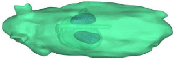
Mouse body with kidney and heart.

The exact solution is designed as

$$u(x,y,z)=\{\begin{array}{ll}10\hfill & \text{in}{\Omega }_1\hfill \\ cos(\omega x)cos(\omega y)cos(\omega z)\hfill & \text{in}{\Omega }_2\hfill \\ x^2+y^2+z^2\hfill & \text{in}{\Omega }_3\hfill \end{array}$$ (46)

with diffusion coefficients

$$\beta =\{\begin{array}{ll}1.0& \text{in}{\Omega }_1\\ 1.5& \text{in}{\Omega }_2\\ 3.0& \text{in}{\Omega }_3\end{array}$$ (47)

The source term is given by

$$q(x,y,z)=\{\begin{array}{ll}0\hfill & \text{in}{\Omega }_1\hfill \\ 4.5{\omega }^{2}cos(\omega x)cos(\omega y)cos(\omega z)\hfill & \text{in}{\Omega }_2\hfill \\ -18\hfill & \text{in }{\Omega }_3\hfill \end{array}$$ (48)

We first consider a case without the linear term, i.e. μ_a = 0. Owing to the large size of the computation domain and numerous irregular points brought by the complicated interface, the computation is carried out in a high-performance computer. The CPU time for each computation is provided. Our results are presented in Table VIII, with w = 0.5. Second-order convergence is obtained in these results. It is also seen that the accuracy, convergence, and CUP time are similar to those in other test problems. Therefore, the proposed MIB method is not sensitive to the complex geometry.

Table VIII.

Errors of MIB solutions for the mouse model in Case 7(a).

	ω = 0.2				ω = 0.1
Mesh size	L∞ norm	Order	CPU	Mesh size	L∞ norm	Order	CPU
4	9.815 (−2)		4	4	1.478 (−2)		3.8
2	1.917 (−2)	2.4	20	2	2.967 (−3)	2.3	20
1	4.700 (−3)	2.0	157	1	5.354 (−4)	2.5	151

Case 7(b)

In the following, we consider this problem with non-vanishing μ_a values. Two sets of μ_a values are employed. Let us denote the first set as large μ_a

$${\mu }_{\text{a}}(x,y,z)=\{\begin{array}{ll}0& \text{in}{\Omega }_1\\ 0.3& \text{in}{\Omega }_2\\ 0.4& \text{in}{\Omega }_3\end{array}$$ (49)

and the second set as small μ_a

$${\mu }_{\text{a}}(x,y,z)=\{\begin{array}{ll}0& \text{in}{\Omega }_1\\ 0.02& \text{in}{\Omega }_2\\ 0.03& \text{in}{\Omega }_3\end{array}$$ (50)

Here, u and beta are the same as the last case, and the source term g can be derived accordingly. We set $\omega =\frac{1}{2}$ in all these computations. Computational results are given in Table IX with different coefficients μ_a. It can be concluded from Table IX that the MIB is robust for the multi-interface elliptic problem. The larger the coefficients μ_a are, the better are the results for both accuracy and CPU time. This is natural because larger coefficients means that the resulting computation matrix is more diagonally dominant. Therefore, the proposed MIB method works well for the mouse model used in the optical molecular imaging.

Table IX.

Errors of the MIB solutions for the mouse model in Case 7(b).

	Large μa				Small μa
Mesh size	L∞ norm	Order	CPU	Mesh size	L∞ norm	Order	CPU
4	4.969 (−2)		1.5	4	8.964 (−2)		2.5
2	1.040 (−3)	2.3	9	2	2.175 (−2)	2.0	15
1	2.620 (−4)	1.9	63	1	4.671 (−3)	2.2	110

4. Conclusion

This paper explores the usefulness and examines the accuracy of the matched interface and boundary (MIB) method for solving diffusion equation for the optical molecular imaging. In the media of high scattering, the governing radiative transfer equation is reduced to the optical diffusion equation. In the context of biomedical imaging, the optical diffusion equation involves complex geometries, discontinuous coefficients, and geometric singularities. This kind of problems have been previous analyzed by the finite element method (FEM), which is typically designed for smooth interfaces. Geometric singularities and coefficients discontinuity give rise to computational challenges. The goal of the present work is to examine the effectiveness of the proposed MIB method, which is designed for elliptic equations with discontinuous coefficients and singular sources. For arbitrarily complex geometries with sharp-edged and sharp-tipped interfaces, we have demonstrated the designed second-order convergence of the MIB method. For smooth interfaces, fourth-order convergence is achieved. The MIB method has also been tested against the variation of the strength of the linear term in the governing optical diffusion equation. It is found that the MIB method converges faster when the strength increases. For a comparison, the results of the FEM are also presented in some 2D and 3D cases with smooth interfaces and continuous solutions. The FEM slightly outperforms the MIB for continuous solutions and interfaces without geometric singularities in 2D. The proposed MIB method exhibits better performance in 3D cases. In general, the present FEM does not work for problems with discontinuous solutions and/or non-smooth interfaces. In contrast, the proposed MIB works well for these problems in both 2D and 3D. A new MIB scheme that works for general multidomain problems is under our consideration. These problems can be very challenging due to the presence of contact singularities. To our best knowledge, currently, no second-order or better convergent scheme has ever been reported for these problems. On the basis of our promising numerical results, we believe that the proposed method has great potential for biomedical optical imaging, including BLT, fluorescence tomography, and other optical imaging applications.

References

- 1.Jaffer FA, Weissleder R. Molecular imaging in the clinical arena. Journal of the American Medical Association. 2005;293(7):855–862. doi: 10.1001/jama.293.7.855. [DOI] [PubMed] [Google Scholar]
- 2.Thakur M, Lentle BC. Report of a summit on molecular imaging. American Journal of Roentgenology. 2006;186(2):297–299. doi: 10.2214/AJR.06.5020. [DOI] [PubMed] [Google Scholar]
- 3.Weissleder R, Ntziachristos V. Shedding light onto live molecular targets. Nature Medicine. 2003;9(1):123–128. doi: 10.1038/nm0103-123. [DOI] [PubMed] [Google Scholar]
- 4.Wang G, Shen H, Cong W, Zhao S, Wei GW. Temperature modulated bioluminescence tomography. Optics Express. 2006;14(17):7852–7871. doi: 10.1364/oe.14.007852. [DOI] [PubMed] [Google Scholar]
- 5.Contag CH, Ross BD. It's not just about anatomy: in vivo bioluminescence imaging as an eyepiece into biology. Journal of Magnetic Resonance Imaging. 2002;16(4):378–387. doi: 10.1002/jmri.10178. [DOI] [PubMed] [Google Scholar]
- 6.Ntziachristos V, Ripoll J, et al. Looking and listening to light: the evolution of whole-body photonic imaging. Nature Biotechnology. 2005;23(3):313–320. doi: 10.1038/nbt1074. [DOI] [PubMed] [Google Scholar]
- 7.So MK, Xu C, et al. Self-illuminating quantum dot conjugates for in vivo imaging. Nature Biotechnology. 2006;24:339–343. doi: 10.1038/nbt1188. [DOI] [PubMed] [Google Scholar]
- 8.Wang G, Hoffman EA, et al. Systems and methods for bioluminescent computed tomographic reconstruction U.S.A. Patent disclosure filed with University of Iowa Research Foundation in July 2002; U.S. provisional patent application filed in March 2003; U.S. patent application filed in March 2004
- 9.Cong A, Wang G. A finite-element-based reconstruction method for 3D fluorescence tomography. Optics Express. 2005;13(24):9847–9857. doi: 10.1364/opex.13.009847. [DOI] [PubMed] [Google Scholar]
- 10.Cong WX, Wang G. Practical reconstruction method for bioluminescence tomography. Optics Express. 2005;13(18):6756–6771. doi: 10.1364/opex.13.006756. [DOI] [PubMed] [Google Scholar]
- 11.Wang G, Hoffman EA, et al. Development of the first bioluminescent CT scanner. Radiology. 2003;299:566. [Google Scholar]
- 12.Wang G, Li Y, et al. Uniqueness theorems in bioluminescence tomography. Medical Physics. 2004;31(8):2289–2299. doi: 10.1118/1.1766420. [DOI] [PubMed] [Google Scholar]
- 13.Ben Ameur H, Burger M, Hackl B. Level set methods for geometric inverse problems in linear elasticity. Inverse Problems. 2004;20:673–696. [Google Scholar]
- 14.Berthelsen PA. A decomposed immersed interface method for variable coefficient elliptic equations with non-smooth and discontinuous solutions. Journal of Computational Physics. 2004;197:364–386. [Google Scholar]
- 15.Biros G, Ying LX, Zorin D. A fast solver for the Stokes equations with distributed forces in complex geometries. Journal of Computational Physics. 2004;193:317–348. [Google Scholar]
- 16.Dumett MA, Keener JP. An immersed interface method for solving anisotropic elliptic boundary value problems in three dimensions. SIAM Journal on Scientific Computing. 2003;25:348–367. [Google Scholar]
- 17.Fogelson AL, Keener JP. Immersed interface methods for Neumann and related problems in two and three dimensions. SIAM Journal on Scientific Computing. 2000;22:1630–1654. [Google Scholar]
- 18.Gibou F, Fedkiw RP. A fourth order accurate discretization for the Laplace and heat equations on arbitrary domains, with applications to the Stefan problem. Journal of Computational Physics. 2005;202:577–601. [Google Scholar]
- 19.Hou S, Liu XD. A numerical method for solving variable coefficient elliptic equation with interfaces. Journal of Computational Physics. 2005;202:411–445. [Google Scholar]
- 20.Hou TY, Li ZL, Osher S, Zhao H. A hybrid method for moving interface problems with application to the Hele–Shaw flow. Journal of Computational Physics. 1997;134:236–252. [Google Scholar]
- 21.Huang H, Li ZL. Convergence analysis of the immersed interface method. IMA Journal of Numerical Analysis. 1999;19:583–608. [Google Scholar]
- 22.Hunter JK, Li ZL, Zhao H. Reactive autophobic spreading of drops. Journal of Computational Physics. 2002;183:335–366. [Google Scholar]
- 23.Jin S, Wang XL. Robust numerical simulation of porosity evolution in chemical vapor infiltration II. Two-dimensional anisotropic fronts. Journal of Computational Physics. 2002;179:557–577. [Google Scholar]
- 24.Johansen H, Colella P. A Cartesian grid embedding boundary method for Poisson's equation on irregular domains. Journal of Computational Physics. 1998;147:60–85. [Google Scholar]
- 25.Kandilarov JD. Immersed interface method for a reaction–diffusion equation with a moving own concentrated source. Lecture Notes in Computer Science. 2003;2542:506–513. [Google Scholar]
- 26.Lee L, LeVeque RJ. An immersed interface method for incompressible Navier–Stokes equations. SIAM Journal on Scientific Computing. 2003;25:832–856. [Google Scholar]
- 27.Li ZL, Lubkin SR. Numerical analysis of interfacial two-dimensional Stokes flow with discontinuous viscosity and variable surface tension. International Journal for Numerical Methods in Fluids. 2001;37:525–540. [Google Scholar]
- 28.Li ZL, Wang WC, Chern IL, Lai MC. New formulations for interface problems in polar coordinates. SIAM Journal on Scientific Computing. 2003;25:224–245. [Google Scholar]
- 29.Linnick MN, Fasel HF. A high-order immersed interface method for simulating unsteady incompressible flows on irregular domains. Journal of Computational Physics. 2005;204:157–192. [Google Scholar]
- 30.Lombard B, Piraux J. How to incorporate the spring-mass conditions in finite-difference schemes. SIAM Journal on Scientific Computing. 2003;24:1379–1407. [Google Scholar]
- 31.Schulz M, Steinebach G. Two-dimensional modelling of the river Rhine. Journal of Computational and Applied Mathematics. 2002;145:11–20. [Google Scholar]
- 32.Sethian JA, Wiegmann A. Structural boundary design via level set and immersed interface methods. Journal of Computational Physics. 2000;163:489–528. [Google Scholar]
- 33.Tornberg AK, Engquist B. Numerical approximations of singular source terms in differential equations. Journal of Computational Physics. 2004;200:462–488. [Google Scholar]
- 34.Voorde JV, Vierendeels J, Dick E. Flow simulations in rotary volumetric pumps and compressors with the fictitious domain method. Journal of Computational and Applied Mathematics. 2004;168:491–499. [Google Scholar]
- 35.Walther JH, Morgenthal G. An immersed interface method for the vortex-in-cell algorithm. Journal of Turbulence. 2002;3 Art. No. 039. [Google Scholar]
- 36.Wiegmann A, Bube KP. The explicit-jump immersed interface method: finite difference methods for PDEs with piecewise smooth solutions. SIAM Journal on Numerical Analysis. 2000;37:827–862. [Google Scholar]
- 37.Fadlun EA, Verzicco R, Orlandi P, Mohd-Yusof J. Combined immersed-boundary finite-difference methods for three-dimensional complex flow simulations. Journal of Computational Physics. 2000;161:30–60. [Google Scholar]
- 38.Francois M, Shyy W. Computations of drop dynamics with the immersed boundary method, part 2: drop impact and heat transfer. Numerical Heat Transfer Part B—Fundamentals. 2003;44:119–143. [Google Scholar]
- 39.Francois M, Uzgoren E, Jackson J, Shyy W. Multigrid computations with the immersed boundary technique for multiphase flows. International Journal of Numerical Methods for Heat and Fluid Flow. 2004;14:98–115. [Google Scholar]
- 40.Iaccarino G, Verzicco R. Immersed boundary technique for turbulent flow simulations. Applied Mechanics Reviews. 2003;56:331–347. [Google Scholar]
- 41.Mittal R, Iaccarino G. Immersed boundary methods. Annual Review of Fluid Mechanics. 2005;37:236–261. [Google Scholar]
- 42.Hadley GR. High-accuracy finite-difference equations for dielectric waveguide analysis I: uniform regions and dielectric interfaces. Journal of Lightwave Technology. 2002;20:1210–1218. [Google Scholar]
- 43.Hesthaven JS. High-order accurate methods in time-domain computational electromagnetics. A review. Advances in Imaging and Electron Physics. 2003;127:59–123. [Google Scholar]
- 44.Kafafy R, Lin T, Lin Y, Wang J. Three-dimensional immersed finite element methods for electric field simulation in composite materials. International Journal for Numerical Methods in Engineering. 2005;64:940–972. [Google Scholar]
- 45.Horikis TP, Kath WL. Modal analysis of circular Bragg fibers with arbitrary index profiles. Optics Letters. 2006;31:3417–3419. doi: 10.1364/ol.31.003417. [DOI] [PubMed] [Google Scholar]
- 46.Liu WK, Liu Y, Farrell D, Zhang L, Wang X, Fukui Y, Patankar N, Zhang Y, Bajaj C, Chen X, Hsu H. Immersed finite element method and its applications to biological systems. Computer Methods in Applied Mechanics and Engineering. 2006;195:1722–1749. doi: 10.1016/j.cma.2005.05.049. [DOI] [PMC free article] [PubMed] [Google Scholar]
- 47.Geng WH, Yu SN, Wei GW. Treatment of charge singularities in implicit solvent models. Journal of Chemical Physics. 2007;127:114106. doi: 10.1063/1.2768064. [DOI] [PubMed] [Google Scholar]
- 48.Yu SN, Geng WH, Wei GW. Treatment of geometric singularities in implicit solvent models. Journal of Chemical Physics. 2007;126:244108. doi: 10.1063/1.2743020. [DOI] [PubMed] [Google Scholar]
- 49.Zhou YC, Feig M, Wei GW. Highly accurate biomolecular electrostatics in continuum dielectric environments. Journal of Computational Chemistry. 2008;29:87–97. doi: 10.1002/jcc.20769. [DOI] [PubMed] [Google Scholar]
- 50.Peskin CS. Numerical analysis of blood flow in heart. Journal of Computational Physics. 1977;25:220–252. [Google Scholar]
- 51.Peskin CS. Lectures on mathematical aspects of physiology. Lectures in Applied Mathematics. 1981;19:69–107. [Google Scholar]
- 52.Peskin CS, Mcqueen DM. A 3-dimensional computational method for blood-flow in the heart. 1. Immersed elastic fibers in a viscous incompressible fluid. Journal of Computational Physics. 1989;81:372–405. [Google Scholar]
- 53.Griffith BE, Peskin CS. On the order of accuracy of the immersed boundary method: higher order convergence rates for sufficiently smooth problems. Journal of Computational Physics. 2005;208:75–105. [Google Scholar]
- 54.Lai MC, Peskin CS. An immersed boundary method with formal second-order accuracy and reduced numerical viscosity. Journal of Computational Physics. 2000;160:705–719. [Google Scholar]
- 55.Fedkiw RP, Aslam T, Merriman B, Osher S. A non-oscillatory Eulerian approach to interfaces in multimaterial flows (the ghost fluid method) Journal of Computational Physics. 1999;152:457–492. [Google Scholar]
- 56.Liu XD, Fedkiw RP, Kang M. A boundary condition capturing method for Poisson's equation on irregular domains. Journal of Computational Physics. 2000;160:151–178. [Google Scholar]
- 57.Babus̆ka I. The finite element method for elliptic equations with discontinuous coefficients. Computing. 1970;5:207–213. [Google Scholar]
- 58.Bramble J, King J. A finite element method for interface problems in domains with smooth boundaries and interfaces. Advances in Computational Mathematics. 1996;6:109–138. [Google Scholar]
- 59.Li ZL, Lin T, Wu XH. New Cartesian grid methods for interface problems using the finite element formulation. Numerische Mathematik. 2003;96:61–98. [Google Scholar]
- 60.Cai W, Deng SZ. An upwinding embedded boundary method for Maxwell's equations in media with material interfaces: 2D case. Journal of Computational Physics. 2003;190:159–183. [Google Scholar]
- 61.Oevermann M, Klein R. A Cartesian grid finite volume method for elliptic equations with variable coefficients and embedded interfaces. Journal of Computational Physics. 2006;219:749–769. [Google Scholar]
- 62.Mayo A. The fast solution of Poisson's and the biharmonic equations on irregular regions. SIAM Journal on Numerical Analysis. 1984;21:285–299. [Google Scholar]
- 63.Mayo A, Greenbaum A. Fourth order accurate evaluation of integrals in potential theory on exterior 3D regions. Journal of Computational Physics. 2007;220:900–914. [Google Scholar]
- 64.Mckenney A, Greengard L, Mayo A. A fast Poisson solver for complex geometries. Journal of Computational Physics. 1995;118:348–355. [Google Scholar]
- 65.LeVeque RJ, Li ZL. The immersed interface method for elliptic equations with discontinuous coefficients and singular sources. SIAM Journal on Numerical Analysis. 1994;31:1019–1044. [Google Scholar]
- 66.Li ZL. A fast iterative algorithm for elliptic interface problems. SIAM Journal on Numerical Analysis. 1998;35:230–254. doi: 10.1137/15M1040244. [DOI] [PMC free article] [PubMed] [Google Scholar]
- 67.Li ZL, Ito K. Maximum principle preserving schemes for interface problems with discontinuous coefficients. SIAM Journal on Scientific Computing. 2001;23:339–361. [Google Scholar]
- 68.Adams L, Li ZL. The immersed interface/multigrid methods for interface problems. SIAM Journal on Scientific Computing. 2002;24:463–479. [Google Scholar]
- 69.Deng SZ, Ito K, Li ZL. Three-dimensional elliptic solvers for interface problems and applications. Journal of Computational Physics. 2003;184:215–243. [Google Scholar]
- 70.Zhao S, Wei GW. High order FDTD methods via derivative matching for Maxwell's equations with material interfaces. Journal of Computational Physics. 2004;200:60–103. [Google Scholar]
- 71.Zhou YC, Zhao S, Feig M, Wei GW. High order matched interface and boundary (MIB) schemes for elliptic equations with discontinuous coefficients and singular sources. Journal of Computational Physics. 2006;213:1–30. [Google Scholar]
- 72.Zhou YC, Wei GW. On the fictitious-domain and interpolation formulations of the matched interface and boundary (MIB) method. Journal of Computational Physics. 2006;219:228–246. [Google Scholar]
- 73.Zhao S, Wei GW, Xiang Y. DSC analysis of free-edged beams by an iteratively matched boundary method. Journal of Sound and Vibration. 2005;284:487–493. [Google Scholar]
- 74.Yu SN, Wei GW. Three dimensional matched interface and boundary (MIB) method for geometric singularities. Journal of Computational Physics. 2007;227:602–632. [Google Scholar]
- 75.Miniowitz R, Webb JP. Covariant-projection quadrilateral elements for the analysis of wave-guides with sharp edges. IEEE Transactions on Microwave Theory and Techniques. 1991;39:501–505. [Google Scholar]
- 76.Caorsi S, Pastorino M, Raffetto M. Electromagnetic scattering by a conducting strip with a multilayer elliptic dielectric coating. IEEE Transactions on Electromagnetic Compatibility. 1999;41:335–343. [Google Scholar]
- 77.Pan G, Tong M, Gilbert B. Multiwavelet based moment method under discrete Sobolev-type norm. Microwave and Optical Technology Letters. 2004;40:47–50. [Google Scholar]
- 78.Pantic-Tanner Z, Savage JZ, Tanner DR, Peterson AF. Two-dimensional singular vector elements for finite-element analysis. IEEE Transactions on Microwave Theory and Techniques. 1998;46:178–184. [Google Scholar]
- 79.van Rens BJE, Brekelmans WAM, Baaijens FPT. Modelling friction near sharp edges using a Eulerian reference frame: application to aluminium extrusion. International Journal for Numerical Methods in Engineering. 2002;54:453–471. [Google Scholar]
- 80.Macak EB, Munz WD, Rodenburg JM. Plasma-surface interaction at sharp edges and corners during ion-assisted physical vapor deposition. Part I: edge-related effects and their influence on coating morphology and composition. Journal of Applied Physics. 2003;94:2829–2836. [Google Scholar]
- 81.Baetke F, Werner H, Wengle H. Numerical-simulation of turbulent-flow over surface-mounted obstacles with sharp edges and corners. Journal of Wind Engineering and Industrial Aerodynamics. 1990;35:129–147. [Google Scholar]
- 82.Cendes ZJ, Shenton DN, Shahnasser H. Magnetic field computation using Delaney triangulation and complementary finite element methods. IEEE Transactions on Magnetics. 1983;19:2251–2554. [Google Scholar]
- 83.Babus̆ka I, Sauter SA. Is the pollution effect of the FEM avoidable for the Helmholtz equation considering high wave number. SIAM Journal on Numerical Analysis. 1997;34:2392–2423. [Google Scholar]
- 84.Yu SN, Zhou YC, Wei GW. Matched interface and boundary (MIB) method for elliptic problems with sharp-edged interfaces. Journal of Computational Physics. 2007;224:729–756. [Google Scholar]
- 85.Arridge AR. Optical tomography in medical imaging. Inverse Problems. 1999;15:R41–R93. [Google Scholar]
- 86.Ishimaru A. Wave Propagation and Scattering in Random Media. Wiley/IEEE Press; New York: 1999. (IEEE Press Series on Electromagnetic Wave Theory). [Google Scholar]
- 87.Klose AD, Hielscher AH. Quasi-Newton methods in optical tomographic image reconstruction. Inverse Problems. 2003;19(12):387–409. [Google Scholar]
- 88.Natterer F, Wubbeling F. Marching schemes for inverse acoustic scattering problems. Numerische Mathematik. 2005;100(4):697–710. [Google Scholar]
- 89.Chen Z, Zou J. Finite element methods and their convergence for elliptic and parabolic interface problems. Numerische Mathematik. 1998;79:175–202. [Google Scholar]
- 90.Fornberg B. Calculation of weights in finite difference formulas. SIAM Review. 1998;40:685–691. [Google Scholar]