An image-driven parameter estimation problem for a reaction-diffusion glioma growth model with mass effects

Abstract

We present a framework for modeling gliomas growth and their mechanical impact on the surrounding brain tissue (the so-called, mass-effect). We employ an Eulerian continuum approach that results in a strongly coupled system of nonlinear Partial Differential Equations (PDEs): a reaction-diffusion model for the tumor growth and a piecewise linearly elastic material for the background tissue. To estimate unknown model parameters and enable patient-specific simulations we formulate and solve a PDE-constrained optimization problem. Our two main goals are the following: (1) to improve the deformable registration from images of brain tumor patients to a common stereotactic space, thereby assisting in the construction of statistical anatomical atlases; and (2) to develop predictive capabilities for glioma growth, after the model parameters are estimated for a given patient. To our knowledge, this is the first attempt in the literature to introduce an adjoint-based, PDE-constrained optimization formulation in the context of image-driven modeling spatio-temporal tumor evolution. In this paper, we present the formulation, and the solution method and we conduct 1D numerical experiments for preliminary evaluation of the overall formulation/methodology.

1 Introduction

Primary brain tumors constitute a significant health challenge, due to their grim prognosis. More than 50% of primary brain tumors are gliomas. Gliomas are seldom treatable with resection and ultimately progress to high-grade, leading to death in only 6-12 months [1]. Despite efforts of the clinical and research communities to improve these statistics, little has been achieved in the past decades in terms of improving treatment of brain tumors, while frequency of brain tumors seems to be increasing.

One of the fundamental difficulties in treating gliomas is their highly diffusive nature and ability to infiltrate healthy tissue well beyond the bulk tumor boundary seen in various imaging modalities. Due to this highly invasive behavior, radical resection of gliomas rarely leads to cure, since cancer cells that have invaded adjacent healthy tissue proliferate at rates that can reach doubling times of 1 week at advanced stages [1], and quickly spread the disease to tissue that can be distant to the original tumor mass, especially if cancer cells find natural pathways of higher diffusivity, such as white matter fiber tracts [2], [3], [4].

Whenever the tumor is not proximal to eloquent areas a margin of normal-appearing tissue surrounding the tumor can be treated together with the cancer itself for preventive reasons. This approach is often over-conservative and highly empirical, partly due to the lack of availability of systematic quantitative approaches to characterizing the spatially heterogeneous patterns of cancer progression, and determining tissue that is likely to be infiltrated and display cancer recurrence. Therefore, there is need for a better understanding of the spatio-temporal progression of brain cancer, and for determining predictive factors for cancer invasion, using phenotypic cancer profiles derived from imaging, histopathology, and potentially other sources, in conjunction with relevant genotypic characteristics. Such predictive factors would allow us to apply more aggressive spatially adaptive treatments.

There has been significant effort to develop mathematical tools that simulate tumor evolution, and to help quantify the impact of various treatments (surgery, chemotherapy, radiotherapy) on the tumor and on the host. Simulation tools based on mathematical modeling have the potential to create a framework for understanding, organizing and applying experimental data acquired during laboratory or clinical studies. Two major approaches are traditionally highlighted in modeling tumor growth: discrete models [5], [6] and continuous hypothesis based models [7]. Recently, hybrid formulations have been investigated [8], [9].

The continuous hypothesis along with macroscopic conservation laws (mass, momentum) translates into a set of partial differential equations. These equations involve a reaction-diffusion framework [10], [11], [12]. Some recent continuous models are multiphase, and account for cellular heterogeneity and mechanical effects [13], [14]. Cellular Automata (CA) models treat the discrete nature of the actual cells realistically, and offer good local adaptability in complex situations. Continuous models, on the other hand, may offer more generality and computational tractability. A mechanical approach has also been attempted to account for the macroscopic growth of tumors and its impact on the surrounding normal parenchyma [15], [16].

Regardless of their particular nature, all tumor growth models involve a number of parameters (the more complex the model, the larger the number of parameters) whose estimation for actual simulation purposes remains a difficult issue. Some attempts have been made [11] to use patient-specific imaging information. One main limitation is the lack of extensive and systematic fitting of these models using large numbers of in vivo patient data, as well as the evaluation of their predictive power on independent datasets.

Imaging plays an important role in diagnosis, treatment, and follow-up of brain cancer. Conventional imaging methods, such as MRI T1-(with and without gadolinium) and T2-weighted sequences, are generally limited to highlighting the bulk of the main tumor mass, and the surrounding mixture of healthy tissue with invading cancer and edema. Less conventional methods, such as perfusion and spectroscopy, are very promising techniques carrying complementary information related to vascularization and tumor biochemistry, respectively. Finally, Diffusion Tensor Imaging (DTI) provides additional information about the structural changes and displacement of major white matter fiber tracts caused by brain tumors.

Contributions

In this article we propose a framework for modeling gliomas growth and the subsequent mechanical impact on the surrounding brain tissue (mass-effect), with estimation of unknown parameters via PDE-constrained optimization. We target a medical imaging context, where such a framework primarily aims at the following goals: (1) improving the deformable registration from the brain tumor patient image to a common stereotactic space (atlas); and (2) developing predictive capabilities for glioma growth. The first is important for integrative statistical analysis of tumors in groups of patients and surgical planning. The second is important for general treatment planning and prognosis. Both are long-term goals.

One of the main interests of this article is the experimental comparison of solution algorithms for the parameter estimation problem associated with the tumor growth and the associated mass-effect. Deformation (compression) of the neighboring tissue induced by tumor growth is commonly referred to as mass-effect. This is a crucial phenomenon, which occurs in the majority of brain-tumor patients and causes distortions (mild to severe) in the various structures (e.g., ventricles, white matter tracts, etc.); it is visible at imaging and well-documented in the medical literature. The importance of modeling and simulating it for the purpose of aiding registration and subsequent surgery/treatment planning has been addressed in detail in a series of publications [16, 17, 18, 19, 20, 21].

In our approach, glioma growth is modeled via a nonlinear reaction-advection-diffusion equation, with a two-way coupling with the underlying tissue elasticity equations. Our formulation is fully Eulerian and naturally allows for updating the tumor diffusion coefficient following structural displacements caused by tumor growth/infiltration. The overall model is governed by a strongly coupled nonlinear system of partial differential equations, which makes the numerical solution procedure quite challenging. In a recent companion piece [22], we employed this model and we solved parameter estimation problems for a handful of tumor parameters using a direct search method. We did not use sophisticated optimization formulations there, but rather we assessed the performance of our model on real brain tumor data from 3D MR images. We illustrate this briefly with an example of such simulations on real brain tumor patient data in section 6.

In the present paper, we are concerned with developing an adjoint-based PDE-constrained formulation and assessing the feasibility of using it to invert for a larger number of tumor parameters (e.g., initial location and profile) in an algorithmically scalable manner. To our knowledge, this is the first attempt in the literature to introduce a PDE-constrained optimization formulation in the context of image-driven modeling of spatio-temporal tumor evolution. The work presented is dedicated to overall formulation/methodology, with emphasis on preliminary analysis and evaluations.

In the inverse estimation phase, we seek find the best set of parameters of a tumor growth model that fits patient-specific data (e.g., images). However, complex models involve a large number of unknown parameters, which makes them difficult to calibrate in a clinical setting give the very sparse data (only one or a few scans per patient.) Here, we choose the simplest model possible with a number of parameters that could be realistically determined and validated from existing data via inverse estimation. We would like to capture the spatio-temporal spread of gliomas and subsequent mass effects (mechanical deformations from tumor growth). ¹

The paper is organized as follows: section 2 introduces the tumor growth model (forward problem), in a fully Eulerian description. Section 3 addresses the associated optimization problem, formulated as a PDE-constrained optimization (inverse problem). The numerical approximation and solution is discussed in section 4. In section 5 we discuss numerical experiments and discuss the feasibility of our framework, while section 6 briefly illustrates some of our simulations on real brain tumor patient data.

2 Modeling growth of gliomas

Continuous model

Our primary focus is on biophysical tumor models that can capture the mass-effect caused by invasion and infiltration. In [17], we have employed a purely biomechanical tumor model to simulate tumor mass-effect in 3D MR images. Here we incorporate more physically-realistic tumor growth models with the assumption that such models may improve predictive capabilities. The modeling framework consists of a reactive-advective-diffusive mass transport for the tumor cells, coupled with elasticity for the brain. ([10], [20], [23]) The mechanical coupling is assumed to be by means of a local pressure field, which is a (parameterized) function of the tumor cell density [15], [20].

Let ω denote the (fixed) spatial domain occupied by the brain and (0, T) a specified time interval. Let U = ω × (0, T). Without regard to tumor cell heterogeneity, let c = c(x, t) denote the local density of tumor cells. The general mass balance for the tumor then reads:

$$\underset{\mathit{rate\; of\; change}}{\underbrace{\frac{\partial c}{\partial t}}}=\underset{\mathit{diffusion}}{\underbrace{\nabla \cdot (D\nabla c)}}-\underset{\mathit{advection}}{\underbrace{\nabla \cdot (c\mathbf{v})}}+\underset{\mathit{reaction}}{\underbrace{r(c)}}\mathrm{in}U,$$ (1)

Here r(c) is a function representing a reactive term that primarily accounts for tumor cell proliferation and death; and D is the diffusion coefficient of tumor cells in brain tissue. Experimental evidence [24] suggests that tumor diffusion may be transversely isotropic in the white matter and isotropic in the grey matter. Here, for simplicity, we shall consider the case of isotropic diffusion in both the white and the grey matter, with diffusion coefficients D_w and D_g, respectively. The tumor cell drift velocity v in equation (1) may well depend on tumor specific mechanisms (chemotaxis, etc. [25]) in reality. In our simplified Eulerian framework, however, it only accounts for the tumor cells being displaced as a consequence of the underlying tissue mechanical deformation (e.g., mass-effect). This velocity field will be defined in what follows.

In an Eulerian frame of reference, regarding the brain as a deformable solid occupying the bounded region ω in space, its motion is described by the following general set of equations:

$$\rho \dot{\mathbf{v}}=\nabla \cdot \mathbf{T}+\mathbf{b}\mathrm{in}U,\mathrm{momentum}$$ (2)

$$\mathbf{T}=\widehat{\mathbf{T}}(\mathbf{F},\dot{\mathbf{F}})\mathrm{in}U,\mathrm{constitutive}$$ (3)

$$\dot{\mathbf{F}}=\nabla \mathbf{vF},\mathbf{v}=\dot{\mathbf{u}}\mathrm{in}U,\mathrm{kinematics}$$ (4)

$$\dot{\mathbf{m}}=0\mathrm{in}U,\mathrm{material\; properties}.$$ (5)

Here v is the (Eulerian) velocity field, u is the displacement field, T is the Cauchy stress tensor and T̂ denotes the constitutive law depending on the deformation tensor F = I + ∇u and its material time derivative Ḟ. b in the momentum conservation equation represents distributed forces. Here m denotes material properties (e.g., Lame’s coefficients in linear elasticity, and the diffusion coefficient D) that are advected with the underlying material motion. The material time derivative operator of a field (scalar, vector, tensor) f is

$$\dot{\mathbf{f}}=\frac{\partial \mathbf{f}}{\partial t}+(\nabla \mathbf{f})\mathbf{v}.$$ (6)

We assume that the forces b are pressure-like, directly proportional to the local gradient of the tumor cell density [15], [20]:

$$\mathbf{b}=-f(c,\mathbf{p})\nabla c,$$ (7)

where f is a strictly positive p-parameterized function introduced to regulate the strength/location of the tumor-induced tissue deformation. Equations (1)-(5) augmented with appropriate initial conditions for c, u, v, F, m and boundary conditions for c, T, u respectively, constitute a coupled, nonlinear system of PDEs.

Additional modeling assumptions

A basic model for the reactive term r(c) in the general diffusion equation (1) can be formulated in terms of growth (cell mitosis) - characterized by a growth rate a and competition for resources - characterized by a competition parameter b: r(c, a, b) = ac − bc². Here, we shall consider an even more particular form. We introduce a threshold value for the tumor cell density - let it be denoted by c_s, a positive constant corresponding to a saturation level. Then the bulk part of the tumor is assumed to be characterized by spatial regions where c ≅ c_s. More refined distinctions within the tumor region are possible through additional corresponding thresholding. Let $\overline{c}=\frac{c}{c_s}$ denote a normalized tumor cell density. For simplicity, in everything that follows we shall continue to employ the notation c instead of c̄, from here on regarded as a normalized tumor cell density. All the terms involving c in (1) and (7) shall be assumed correspondingly scaled. Then let:

$$r(c,\rho )=\rho c(1-c).$$ (8)

Thus, in regions where c ≪ 1 (infiltration), the customary proliferation term ρc corresponding to exponential growth at rate ρ is retrieved [10]. Proliferation is assumed to slow down in regions with c getting closer to 1 (tumor bulk), and it eventually becomes a death term if c becomes larger than 1. For simplicity, we shall employ the linear elasticity theory and approximate the brain tissue as a linear elastic inhomogeneous material:

$$\mathbf{T}=\mathit{\sigma }=(\lambda \nabla \cdot \mathbf{u})+\mu (\nabla \mathbf{u}+\nabla {\mathbf{u}}^T),$$ (9)

where λ and μ are the spatially varying Lame’s coefficients (related to Young’s modulus E and Poisson’s ratio ν). The simplest possible candidate for the function f(c, p) in (7) is a positive (a priori unknown) constant. However, such a choice does not allow for much flexibility in capturing both strong tumor mass-effect (generally caused by the tumor bulk) and milder mass-effects (generally caused by tumor infiltration). While various other possibilities exist, here a smooth expression for f(c, p) is suggested, of the form

$$f(c,\mathbf{p})=p_1{e}^{-\frac{p_2}{c^s}}{e}^{-\frac{p_2}{{(2-c)}^s}},$$ (10)

where p = (p₁, p₂, s) and p₁, p₂, s are positive constants. This function is monotonically increasing for 0 < c ≤ 1 and has a maximum at c = 1, which corresponds to the tumor bulk part. The parameter p₂ regulates both the spatial location and the strength of the mechanical deformation caused by the tumor, while p₁ is simply a scaling factor.

Remark

since the bulk tumor is characterized by c ≅ 1, we assume that the maximum tumor cell density does not deviate significantly from 1.

Let us summarize the coupled system of PDEs governing our deformable model for simulating glioma growth:

$$\frac{\partial c}{\partial t}-\nabla \cdot (D\nabla c)+\nabla \cdot (c\mathbf{v})-\rho c(1-c)=0$$ (11)

$$\nabla \cdot ((\mathrm{\lambda }\nabla \cdot \mathbf{u})+\mu (\nabla \mathbf{u}+\nabla {\mathbf{u}}^T))-f(c,\mathbf{p})\nabla c=0$$ (12)

$$\mathbf{v}=\frac{\partial \mathbf{u}}{\partial t}$$ (13)

$$\frac{\partial \mathbf{m}}{\partial t}+(\nabla \mathbf{m})\mathbf{v}=0$$ (14)

The reduced expression (13) of the Eulerian velocity field v holds in the linear theory, under the assumption of small strains. Also, given the actual tumor growth scale (cell mitosis), the mechanical deformation may be approximated as a quasi-static process, which explains the absence of the inertial term in the momentum conservation equation (12). For concision, we used the collective notation m = (λ, μ, D) in equation (14). Elastic material properties λ and μ are advected due to the assumption of brain tissue elastic inhomogeneity. The advection equation for the diffusion coefficient D has been written with the assumption in mind that diffusivity of tumor cells is different in white and gray matter respectively; therefore, D must also be updated to reflect the displacement of such structures in the brain.

In a shorthand notation, the system of equations (11)-(14) can be re-written in the following compact form:

$$\frac{\partial \varphi }{\partial t}+\mathbf{A}\varphi +\mathbf{F}(\varphi )=0,$$ (15)

where we introduce the collective notations m = (D, λ, μ) for the material properties and ϕ = (c, u, v, m) for the model state variables. A in equation (15) is a linear differential operator, while the nonlinear function F(ϕ) represents the source/force terms. The following boundary and initial conditions are specified to complete the system of equations (11)-(14):

$$\frac{\partial c}{\partial n}=0\mathrm{on}\partial \omega \times (0,T)$$ (16)

$$\mathbf{u}=0\mathrm{on}\partial \omega \times (0,T)$$ (17)

This implies that

$$\mathbf{v}=0\mathrm{on}\partial \omega \times (0,T).$$ (18)

$$c(\mathbf{x},t=0)=c_0(\mathbf{x})\mathrm{prescribed\; on}\omega$$ (19)

$$\mathbf{u}(\mathbf{x},t=0)=0,\mathbf{v}(\mathbf{x},t=0)=0\mathrm{on}\omega$$ (20)

$$(D,\lambda ,\mu )(\mathbf{x},t=0)=\{\begin{array}{l}(D_w,{\lambda }_w,{\mu }_w),\mathbf{x}\mathrm{in}\mathrm{the}\mathrm{white}\mathrm{matter}\\ (D_g,{\lambda }_g,{\mu }_g),\mathbf{x}\mathrm{in}\mathrm{the}\mathrm{grey}\mathrm{matter}\\ (D_v,{\lambda }_v,{\mu }_v),\mathbf{x}\mathrm{in}\mathrm{the}\mathrm{ventricles}\end{array}$$ (21)

The boundary conditions (16) and (17) come from the assumptions of zero tumor cell flux and zero tissue displacement at the skull. The advection equations (14) are regarded as initial value problems, with the initial values (21) piecewise-constant, assigned from the corresponding segmented MR image [17](see figure 1). Equations (11)-(14) with the boundary and initial conditions (16)-(21) represent a mixed parabolic-elliptic-hyperbolic nonlinear system of PDEs. The numerical solution procedure shall be discussed and illustrated in section 4.

Figure 1.

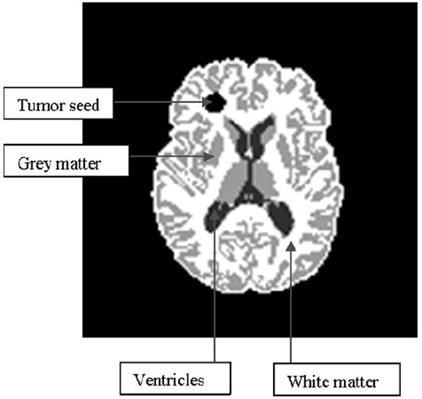
Segmented MR image - axial slice.

3 The inverse problem

Motivation

A few references exist in literature regarding tumor cell diffusivity D_w in white matter and D_g in grey matter, as well as the tumor growth rate ρ [10]. In reality, they are unknown, especially in vivo. Regarding the elastic parameters in equation (12): various values for the elastic material properties E (stiffness) and ν (compressibility) of the brain have been used so far in literature [26]. While for white and grey matter there is a range of values frequently employed in the biomechanics community, there is no established approach for the ventricles or for the tumor. In [17], we modeled the ventricles as a soft material, with reasonable results ². Little is known about material properties of tumors; they should be regarded as unknown parameters as well.

The set of parameters p in (10) introduced to model the mechanical deformation of the brain tissue following tumor growth is also unknown.

Another point of interest is to find the spatial location where the tumor initially originated, based on later MRI scans, which in our model formulation is related to the initial condition (19) on tumor cell density. In medical image analysis, registration of a tumor-bearing patient image with a normal brain template requires estimating an initial tumor seed [27].

Here, we consider the case of available serial scans (3D MR images) for a brain-tumor subject at different moments in time over a time interval of length T. The problem is to find a set of model parameters able to generate images that ‘best match’ the available scans over time (0 < t ≤ T) by applying the model starting from the earliest scan (re-labeled as time t = 0). This translates into a PDE-constrained optimization problem, with the constraints given by the model governing equations (11)-(21). An objective functional that defines a ‘best match’ needs to be constructed.

Note

1. From a practical point of view, serial scans of human subjects with low grade gliomas progressing into higher malignancy are difficult to gather, although some clinical studies have been conducted [28]. These studies are more readily achievable in mouse/rat subjects (e.g. [29]), injected with glioma cells and kept under observation over a time interval (days-weeks), during which successive scans are acquired. Such serial data sets can be employed in conjunction with our proposed framework for a preliminary validation/calibration of the tumor growth model in- vivo.

2. It is likely that in the case of actual human subjects, the earliest scan acquired has a visible tumor seed present. In this case, for completeness, one may consider augmenting the initial condition (21) with (D, λ, μ)(x, t = 0) = (D_tum, λ_tum, μ_tum) for points x in the tumor region. The newly introduced set of model parameters (D_tum, λ_tum, μ_tum) stands for the diffusivity and elastic material coefficients inside the tumor.

The objective functional

One functional can be constructed by matching the spatio-temporal evolution of the (normalized) tumor density c(x, t) predicted by the model with the corresponding tumor probability maps independently estimated by a trained classifier [30] from the available serial scans for one particular subject. Let N ≥ 1 be the number of available scans for the subject under consideration. Given estimates ${\{c_k^{\ast }(\mathbf{x})\}}_{k=1}^N$ of the tumor density at times ${\left\{t_k\right\}}_{k=1}^N$, minimize

$$J=\frac{1}{2}\sum _{k=1}^N{\mathit{\int }}_0^T{\mathit{\int }}_{\omega }\delta (t-t_k){(c(\mathbf{x},t)-c_k^{\ast }(\mathbf{x}))}^{2}d\mathbf{x}dt.$$ (22)

A second candidate for the objective functional is related to landmark registration, a common technique in medical imaging: sets of corresponding landmarks manually tracked in the original scan and in the follow-up target scans by an expert. Let {x_l}_l=1,…,L denote a set of L manually-placed landmarks in the initial scan and ${\{{\mathbf{x}}_l^k\}}_{l=1,\dots ,L;k=1,\dots ,N}$ the corresponding manually-placed landmarks at times ${\left\{t_k\right\}}_{k=1}^N$ in the follow-up target scans. Define

$$J=\frac{1}{2}\sum _{k=1}^N\sum _{l=1}^L{\mathit{\int }}_0^T{\mathit{\int }}_{\omega }\delta (t-t_k)\delta (\mathbf{x}-{\mathbf{x}}_l^k){(\psi (\mathbf{x},t)-{\mathbf{x}}_l)}^{2}d\mathbf{x}dt,$$ (23)

where ψ(x, t) is the solution to the following initial-value problem:

$$\begin{array}{cc}\frac{\partial \psi }{\partial t}+(\nabla \psi )\mathbf{v}& =0\\ \psi (\mathbf{x},t=0)& =\mathbf{x}.\end{array}$$ (24)

The function ψ is introduced in our Eulerian formulation to keep track of the particles of interest (initial given landmarks) over time.

We assume that the initial material properties (elastic material properties and diffusion coefficients) are known. Let the set of inversion variables be g = (ρ, p₁, p₂). The first-order necessary conditions for optimality, or KKT conditions, may be derived by introducing an associated Lagrangian functional

$$L(\varphi ,\mathit{\zeta },\mathit{g})=J+{\mathit{\int }}_U\mathit{\zeta }\cdot (\frac{\partial \varphi }{\partial t}+\mathbf{A}\varphi +\mathbf{F}(\varphi ,\mathit{g}))d\mathbf{x}dt+\frac{a}{2}{\mathit{g}}^T\mathit{g},$$

where ζ represents the adjoint (or dual) variable of the corresponding set of state variables ϕ; g denotes the inversion parameters; and a ≥ 0 denotes a regularization parameter. By requiring stationarity of the Lagrangian functional with respect to the adjoint, state, and inversion variables respectively, we obtain the so-called the KKT optimality conditions [31]:

$$\frac{\delta L}{\delta \mathit{\zeta }}=0\Rightarrow \mathrm{state}\mathrm{equations}$$ (25)

$$\frac{\delta L}{\delta \varphi }=0\Rightarrow \mathrm{adjoint}\mathrm{equations}$$ (26)

$$\frac{\delta L}{\delta \mathit{g}}=0\Rightarrow \mathrm{inversion}\mathrm{equations}$$ (27)

(The notation δL here denotes the first variation of L.) These equations form a set of nonlinear PDEs on the state, adjoint, and inversion parameters respectively. The adjoint equations are given by

$$-\frac{\partial \zeta }{\partial t}+{\mathbf{A}}^{\ast }\mathit{\zeta }+{\mathbf{F}}^{\ast }(\mathit{\zeta },\varphi ,\mathit{g})=0,\zeta (t=T)={\zeta }_0.$$ (28)

Operator A* is the adjoint of the A; F* involves Frechet derivatives of F. The corresponding boundary conditions on the adjoint variable(s) ζ, along with the detailed adjoint and inversion equations can be found in the Appendix. ³:

$$\mathbf{G}(\varphi ,\mathit{\zeta },\mathit{g})=0$$

Let us note that one can include additional constraints on the inversion variables g, for example box constraints. In our implementation we use such box constraints to avoid non-physical values of g. For a discussion on the optimality conditions for the case of inequalities see [32]. In our experiments, the regularization parameter is chosen using a trial-and-error procedure to obtain the minimum discrepancy between the data and the prediction. In general, the choice of the regularization parameter requires quantification of the noise in the data and an iterative procedure, for example, using the Morozov discrepancy-principle approach [33]. This work is a preliminary evaluation of the optimization framework; we have attempted to analyze neither the behavior of the inversion operator nor the effects of noise on the choice of the regularization parameter.

Below we outline the iterative algorithm we use to solve for the optimality conditions (25)-(27).

• Given g, solve the state equations for ϕ:

  $$\frac{\partial \varphi }{\partial t}+\mathbf{A}\varphi +\mathbf{F}(\varphi ,\mathit{g})=0,\varphi (t=0)={\varphi }_0$$
• Given g and ϕ, solve the adjoint equations for ζ:

  $$\frac{\partial \zeta }{\partial t}+{\mathbf{A}}^{\ast }\mathit{\zeta }+{\mathbf{F}}^{\ast }(\mathit{\zeta },\varphi ,\mathit{g})=0,\zeta (t=T)={\zeta }_0$$
• Given ϕ and ζ, solve the inversion equations to update g:

  $$\mathbf{G}(\varphi ,\mathit{\zeta },\mathit{g})=0$$

The adjoint equations (28) (see the detailed equations (A-2) and (A-5), (A-3) in Appendix) are posed backward in time with a terminal condition at t = T, while the state equations are posed forward in time, with an initial condition at t = 0. When one discretizes the coupled optimality system (see Appendix for details), the marching directions in time for the state and the adjoint systems are opposite to each other, therefore the unknowns are coupled at all time levels.

Gradient-based optimization algorithms require the evaluation of the gradient of the functional. There are two customary ways of determining this gradient: sensitivity-based approaches and adjoint-based approaches. Evaluation of the gradient through sensitivities requires solving a number of sensitivity systems equal to the number of inversion variables [31] (per optimization iteration). Evaluating the gradient through adjoints only requires one solve of the adjoint system (per optimization iteration), regardless of the number of inversion variables [31]. Finite differences can be used for gradient approximation, but this is an again an expensive approach: at each optimization iteration it requires a number of the forward problem solves equal to the number of inversion variables.

4 Discretization and Numerical Solution

Our goal is to design efficient and robust schemes for solving both the forward problem (equations (11)-(21)) and the adjoint problem (e.g., equations (A-2)-(A-5) in Appendix). In the present paper we discuss only one dimensional numerical experiments.⁴

The fictitious domain method

Brain has complex geometry. Solving PDE’s in such a domain is challenging. Various techniques exist for solving PDEs in complex domains: unstructured meshes that conform to the irregular domain boundary in finite element methods; immersed interface/ghost-fluid methods in finite volume (FV)/finite difference methods (FD); or integral equation methods. In [17, 34], we successfully employed a fictitious domain. We use a similar approach here. Details on implementing a fictitious domain method in the present context are given in the Appendix.

Numerical approximation: regular grids and fractional time steps

For simplicity, we use an operator-splitting approach for the forward and adjoint problems. The independent operators correspond to the advection, diffusion and reaction processes [35], [36]; and the elasticity operator. Each operator is handled independently. We have implemented the diffusion and elasticity elliptic solvers, and two advection solvers conservative term in the mass transport (the ∇ · (cv) term in (11)) and the other for the non-conservative transport (the (∇ψ)v term in (24)).

Consider the forward problem (11)-(21). Let ϕ = (c, u, v, D, λ, μ) denote the vector of unknowns. Let Δ,A₁,R denote the diffusion, advection and reaction operators in the diffusion equation (11), and A₂ denote the advection operator in equations (14). These operator notations will be preserved in the adjoint problem as well. If ϕⁿ = (cⁿ, uⁿ, vⁿ, Dⁿ,λⁿ, μⁿ) is the solution at time t = t_n, then a simple way to update the solution ϕⁿ⁺¹ at the next time step t_n+1 = t_n + Δt is as follows:

• Solve the advection equations (14) using an explicit upwind scheme over time Δt to obtain (Dⁿ⁺¹, λⁿ⁺¹, μⁿ⁺¹).

• Solve the diffusion equation (11) using a simple fractional step method [35]:

  • Solve $\frac{\partial c}{\partial t}=A_1(c,\mathbf{v})$ over time Δt with data (cⁿ, vⁿ), using an explicit conservative upwind scheme, to obtain c*;
  • Solve $\frac{\partial c}{\partial t}=\mathrm{\Delta }(c,D)$ over time Δt with data (c*, Dⁿ⁺¹), using an implicit scheme, to obtain c**;.
  • Solve $\frac{\partial c}{\partial t}=R(c)$ over time Δt with data c**, using an implicit scheme, to obtain cⁿ⁺¹.

• Solve the elasticity equation (12) with data (cⁿ⁺¹, λⁿ⁺¹, μⁿ⁺¹) to obtain uⁿ⁺¹ and update the velocity vⁿ⁺¹ using backward time-differencing in equation (13).

A similar description of the proposed numerical solution algorithm for the adjoint problem can be found in the Appendix. ⁵

5 Numerical Experiments

In this section, the 1D versions of the forward problem (11)-(21) and adjoint problem (A-2)-(A-5) are employed. In the 1D case, let ω = [x₁, x₂], 0 ≤ x₁ < x₂ < ∞ denote a bounded interval on the real positive axis. ⁶ The 1D version of the elasticity equation (12), with s = 1, reads

$$\frac{\partial }{\partial x}({\mu }_e\frac{\partial u}{\partial x})-p_1{e}^{-\frac{p_2}{c}}{e}^{-\frac{p_2}{(2-c)}}\frac{\partial c}{\partial x}=0\mathrm{in}\omega \times [0,T],$$ (29)

In the inhomogeneous case:

$${\mu }_e(x,t=0)=\{\begin{array}{l}{\mu }_{\mathit{ew}},x\mathrm{in}{S}_1(‘\mathrm{white}\mathrm{matter}’),\\ {\mu }_{\mathit{eg}},x\mathrm{in}{S}_2(‘\mathrm{grey}\mathrm{matter}’),\end{array}$$ (30)

with S₁ and S₂ subsets of the 1D spatial domain ω such that S₁ ∪ S₂ = ω. (The homogeneous case is retrieved by setting μ_e (x, t = 0) = μ_ew in ω.) For convenience here, we choose to further scale μ_e and p₁ in equation (29) by a factor equal to μ_ew. We keep the same notation as in (29), with μ_ew = 1, while the values of μ_eg and p₁ are accordingly scaled. ⁷

Remarks:

• As discussed in [10], the inter-play between the diffusion coefficient D and the tumor growth rate ρ in equation (11) allows the model to simulate multiple tumor grades: high-grade (high ρ and high D), intermediate grade (high ρ and low D or low ρ and high D) and low grade (low ρ and low D). Here, we will also be interested in the corresponding mass-effect exerted by the growing tumor. To have such an effect we use a low D and a (relatively) high ρ combination, which is likely to produce steeper gradients $\frac{\partial c}{\partial x}$ in the force term of the elasticity equation (29).

• In the 1D case, there is no actual need to employ a fictitious domain approach, but we use it here in order to test the proposed approach on model problems.

• The numerical scheme is first-order accurate in space-time (O (Δx, Δt)). This was confirmed in a series of numerical experiments. A set of results can be found in the Appendix. ⁸

Test-cases for the overall optimization framework

In all the test-cases presented here, the following have been commonly used, unless otherwise specified: the physical spatial domain [2, 8] is embedded on the larger fictitious domain (see Appendix) [0, 10]; a uniform spatial discretization with Δx = 10/ 64 and a contrast factor ε = (Δx)² (see below material properties); a time span from [0, T], where T = 360, with a time-step Δt = 0.5; an inhomogeneous material with

$$(D,{\mu }_e)(x,t=0)=\{\begin{array}{cc}\hfill (D_w,{\mu }_{\mathit{ew}}),\hfill & x\in [3.5,6.5]\hfill \\ \hfill (D_g,{\mu }_{\mathit{eg}}),\hfill & x\in [2,3.5)\cup (6.5,8)\hfill \\ \hfill (\epsilon D_g,{\mu }_{\mathit{eg}}/\epsilon ),\hfill & x\in [0,2)\cup (8,10),\hfill \end{array}$$

Here we have set D_w = 0.0001, D_g = 0.00005, μ_ew = 1, μ_eg = 1.2. ⁹. Our implementation is done in MATLAB; we used an in-house optimizer and MATLAB’s Optimization Toolbox. Our goals are to test and evaluate the performance of an adjoint-based optimization method within the proposed framework, in terms of correctness, number of optimization iterations, and scalability with respect to the number of inversion variables.

We have set bounds on the inversion parameters to avoid non-physical values during the course of the optimization iterations. We first optimize using a direct search method, which is a version of the MATLAB simplex-based function ‘fminsearch’, modified to allow bounds. The corresponding run-time for the direct search method is used as benchmark. Our main interest lies in a gradient-based optimization, with the gradient computed via the adjoints. For comparison purposes, we also optimize using a gradient-based method with the gradient computed via finite differences (FD). In both gradient-based optimizations, we use the ‘fmincon’ function in MATLAB, with lower and upper bounds imposed. In our test we only retrieve local minima. The target tumor densities have been chosen either by selecting g and solving for a model-generated density, or by a-priori choosing an “arbitrary” density distribution.

The default value of the regularization parameter for the cases with finite (low)-dimensional optimization parameter was a = 0; however, in the experiments where convergence was observed to be slow or failed to occur after the specified maximum number of iterations, we found a ‘good’ value 0 < a ≤ 0.1 by trial-and-error (bisection-like method), on a case-by-case basis. Here by a ‘good’ value, we understand a value for which the convergence was observed experimentally to improve (in terms of the number of iterations to convergence). For the one infinite-dimensional case we consider (test-case 5 below, where we invert for the initial tumor density regarded as a space-dependent function), the default regularization parameter a needs to be a positive number (also determined by trial-and-error) to result in a well-posed problem [39].

The termination tolerances given in the experiments discussed below correspond to the Matlab built-in options: the termination tolerance on the optimization variable refers to the Matlab option ‘TolX’, while the termination tolerance on the function value to the Matlab option ‘TolFun’. These termination tolerances were varied in all our experiments; however, below the tolerances reported in the text, no significant changes in the optimization results were observed, at the expense of increasing the number of iterations.

• Test-case 1: three parameter (ρ, p₁, p₂) optimization, arbitrary target tumor density. Consider first the case of a Gaussian tumor distribution given by

  $$c^{\ast }(x,t)=\frac{t}{T}{e}^{-{(x-5)}^2},x\in [2,8],t\in [0,T],$$ (31)

  with T = 180. The initial tumor density is prescribed as

  $$c(x,t=0)=\{\begin{array}{cc}0.0001,& x\in [4.75,5.25]\\ 0,& \mathrm{otherwise}.\end{array}$$
  The objective functional in this case is of the form (22):

  $$J_1=\frac{1}{2}{\mathit{\int }}_0^T{\mathit{\int }}_{\omega }{(c(x,t)-c^{\ast }(x,t))}^2\mathit{dxdt}+\frac{a}{2}({\rho }^2+p_1^2+p_2^2).$$

  Here a ≥ 0 is just a regularization parameter; in certain cases, a ‘small’ positive value of a helps convergence—its value is decided by trial-and-error. We want to find the set of model parameters g = (ρ, p₁, p₂) leading to a tumor density c(x, t) that best matches the target tumor density c*(x, t). The results of the optimization procedure are summarized in table 1. The initial guess was set to g₀=(0.001, 0.001, 0.001), and the following lower and upper bounds were imposed: g_min = (0, 0, 0), g_max = (0.5, 1.5, 0.5). The stopping criteria that have been used in all three methods are: termination tolerance on the optimization variable (g) set to 10⁻⁴ and the termination tolerance on the function value set to 10⁻⁴. The regularization parameter here was a = 0. The final value of the objective functional was around 9.51 in all three cases, and the ‘match’ at the final moment of time t = T is shown in figure 2.

• Test-case 2: three parameter (ρ, p₁, p₂) optimization, model-generated target tumor density. Consider now an optimization problem similar to the one in test-case 1, but this time with a target tumor density c*(x, t) generated via the forward problem, for a choice of the three model parameters g = (ρ, p₁, p₂) = (0.05, 1.2, 0.1). The model-generated target tumor density is shown in figure 3, marked with circles. The initial tumor density and objective functional are similar to those in the test-case 1 above. This is a typical test case, where the inverse problem is solved to investigate if/how close the original values of the parameters (ρ, p₁, p₂) can be retrieved. The answer is not obvious, since the solution of the inverse problem might not be unique, on the one hand, and since we are only able to find local minima here, on the other. The results of the optimization procedure for this case are summarized in table 2. The initial guess was g₀=(0.001, 0.001, 0.001), with lower and upper bounds g_min = (0, 0, 0), g_max = (0.5, 1.5, 0.5). The stopping criteria that have been used in all three methods for this case are: termination tolerance on the optimization variable (g) set to 10⁻⁶ and the termination tolerance on the function value set to 10⁻⁶. The regularization parameter here was a = 0 as well. The original parameter values (ρ, p₁, p₂) = (0.05, 1.2, 0.1) were very closely retrieved by all three optimization methods, with final values of the objective functional of the order of 10⁻⁷. As we will see in the test-case 3. following, this is not always the case.

• Test-case 3: three parameter (ρ, p₁, p₂) optimization, model-generated target landmarks. The target landmarks are generated via the forward problem, for a choice of the three model parameters (ρ, p₁, p₂) = (0.05, 1.2, 0.1). For simplicity, we only consider the target landmarks at the final time t = T. We considered a set of eight landmarks. The initial landmark position is given by: {X_l}_l=1,2,…,8 = [3, 4, 4.5, 4.75, 5.25, 5.5, 6, 7] and the corresponding (target) position at t = T, estimated via the forward problem, is {x_l}_j=1,2,…,8 = [2.6955, 3.6963, 4.374, 4.7044, 5.3397, 5.6849, 6.3385, 7.2632]. They are shown in figure 4. The maximum landmark displacement is 0.3386 (cm). The objective functional we consider in this case is of the form (23):

  $$J_2=\frac{1}{2}\sum _{l=1}^8{\mathit{\int }}_{\omega }\delta (x-x_l){(\psi (x,t)-X_l)}^2\mathit{dx}+\frac{a}{2}({\rho }^2+p_1^2+p_2^2).$$

  As in the test-case 2, here we solve the inverse problem to investigate if the original values of the parameters (ρ, p₁, p₂), used in the forward problem to generate the target data, can be retrieved. As discussed in section 3, in this case an additional advection equation (see equation (24)) for the variable ψ must be solved in the forward problem and correspondingly in the adjoint problem (see equation (A-9) in Appendix).

  The results of the optimization are summarized in table 3. The initial guess in this case was g₀=(0.1, 0.1, 0.1), with lower and upper bounds g_min = (0, 0, 0), g_max = (0.5, 1.5, 1.0). The stopping criteria used in all three methods are: 10⁻⁴ for the termination tolerance on the optimization variable and 10⁻⁴ for the termination tolerance on the function value. A good regularization parameter to speed-up convergence here was found (trial-and-error) to be a = 0.001. As it can be seen from table 3, in this case two of the three original parameter values (p₁, p₂) = (1.2, 0.1) were not too closely retrieved by any of the three optimization methods, which did converge with the specified tolerance, yielding final values of the objective functional around 0.03. Strengthening the convergence criteria did not produce significant changes, except increasing the number of iterations. In figure 5, the landmark position at time t = T calculated for the values of the parameters (ρ, p₁, p₂) shown in table 3 is illustrated. The match with the actual target landmarks is very good, with the following maximum (absolute) errors: 0.0157 (cm) for the direct search solution, 0.0194 (cm) for the FD gradient-based solution and 0.0210 (cm) for the adjoint gradient-based solution.

  In this case, the solution of the inverse problem is not unique; in terms of the underlying model physics, the interplay between the elastic force parameters p₁ and p₂ in equation (10) can lead to relatively similar elastic deformations for different sets (p₁, p₂). Unless a global optimizer is employed, one can only guarantee to find local minima. Additional information about the tumor itself, whenever available (e.g., appearance, grade, etc.) should be used to constrain the problem toward sorting out the solution that is most plausible physiologically.

• Test-case 4: six parameter (ρ, p₁, p₂, c₁, c₂, c₃) optimization, model-generated target tumor density. In test-cases 1-3, the initial tumor density was assumed given. Suppose now that in addition to the three parameters (ρ, p₁, p₂) we have optimized for so far, we also want to optimize for the initial tumor seed.

  In practical medical applications such as registration of tumor-bearing brain images, estimation of the initial tumor seed is of importance [27]. In this experiment, the tumor seed is parameterized as

  $$c_0(x)=c(x,t=0)=c_1{e}^{\frac{-{(x-c_2)}^2}{2c_3}},\forall x,$$ (32)

  where (c₁, c₂, c₃) are three a priori unknown parameters, with c₁, c₃ > 0. These three parameters define the initial ‘tumor seed’: c₂ defines the center, c₃ an initial ‘radius’, while c₁ is simply a magnitude scaling factor. This parameterization is a modeling assumption since tumors do have Gaussian distributions in reality.
  As in test-case 2 before, consider again the case of a target tumor density c*(x, t) generated via the forward problem, now for a choice of the six model parameters (ρ, p₁, p₂, c₁, c₂, c₃) = (0.05, 1.2, 0.1, 0.0004, 5, 0.06). The terminal time in this case is T = 300. The objective functional is similar to that in the test-case 2 above, plus an additional regularization term for the three newly introduced parameters:

  $$J_1=\frac{1}{2}{\mathit{\int }}_0^T{\mathit{\int }}_{\omega }{(c(x,t)-c^{\ast }(x,t))}^2\mathit{dxdt}+\frac{a}{2}({\rho }^2+p_1^2+p_2^2+c_1^2+c_2^2+c_3^2).$$
  Accordingly, the inversion equations (A-6) in the Appendix must be augmented with three additional inversion equations, corresponding to the newly introduced parameters (c₁, c₂, c₃):

  $$\begin{array}{c}{\mathit{ac}}_1-{\mathit{\int }}_{\omega }\alpha (x,t=0)\frac{\partial c_0}{\partial c_1}\mathit{dx}=0\\ {\mathit{ac}}_2-{\mathit{\int }}_{\omega }\alpha (x,t=0)\frac{\partial c_0}{\partial c_2}\mathit{dx}=0\\ {\mathit{ac}}_3-{\mathit{\int }}_{\omega }\alpha (x,t=0)\frac{\partial c_0}{\partial c_3}\mathit{dx}=0\end{array}$$

  We solved the inverse problem to investigate if/how close the original values (0.05, 1.2, 0.1, 0.0004, 5, 0.06) of the six parameters (ρ, p₁, p₂, c₁, c₂, c₃) can be retrieved. The results are summarized in table 4. The initial guess was g₀ = (0.001, 0.001, 0.001, 0, 4, 0.001), with lower and upper bounds (0, 0, 0, 0, 4, 0), (0.2, 0.5, 1.5, 0.001, 6, 0.1). The stopping criteria in all three methods were: 10⁻⁶ for the termination tolerance on the optimization variable and 10⁻⁶ for the termination tolerance on the function value. A good value of the regularization parameter for the gradient-based optimization in this case was found (trial-and-error) to be a = 0.005.

  The original parameter values (ρ, p₁, p₂, c₁, c₂, c₃) = (0.05, 1.2, 0.1, 0.0004, 5, 0.06) were closely retrieved by the gradient-based methods, with exit values of the objective functional around 0.06. The direct search method in this case performed poorly.

  For a better assessment of scalability, we repeated the above test, this time keeping the three initial tumor parameters (c₁, c₂, c₃) fixed, with values (0.0004, 5, 0.06), while optimizing for the remaining three: (ρ, p₁, p₂). The initial guess ((0.001, 0.001, 0.001)), the lower/upper bounds ((0, 0, 0) and (0.2, 0.5, 1.5)) and the stopping criteria were kept the same as above. The optimization results are summarized in table 5: Comparing the run times in tables 4 and 5, it is apparent that the adjoint-based method scales best with the number of inversion variables. By “scales”, we mean that the cost of the gradient evaluation is equal to one forward and one adjoint solve, but the cost of the gradient evaluation for the finite-difference requires as many forward solves as the size of the inversion parameters.

• Test-case 5: 18 inversion variables, model-generated target tumor density. We use the same target density as in the test-case 2. In this test, we invert for the initial tumor profile c(x, t = 0) = c₀(x) everywhere in the actual physical domain. The target tumor density is computed using the forward solver in a coarser spatial mesh: Δx = 10/32, corresponding to 33 nodes in the larger embedding domain [0, 10], from which only 18 are actually inside [2, 8]. Δt = 0.5 as before. In this case, we want to invert for the 18 corresponding nodal values of c₀(x).

  The objective functional is:

  $$J_1=\frac{1}{2}{\mathit{\int }}_0^T{\mathit{\int }}_{\omega }{(c(x,t)-c^{\ast }(x,t))}^2\mathit{dxdt}+\frac{a}{2}{\mathit{\int }}_{\omega }{c}_0{(x)}^2\mathit{dx},$$

  (a regularization parameter), with the inversion parameters expressed in terms of the adjoints [31] as:

  $${\mathit{ac}}_0(x)-\alpha (x,t=T)=0,\forall x.$$ (33)

  We started with an initial guess of c₀(x) = 0, ∀x; the lower bounds were set equal to 0 everywhere, while the upper bounds were set to 1 inside the actual physical domain [2, 8] and 0 outside, in the fictitious domain. The regularization parameter here was a = 0.1 and the stopping criteria 10⁻⁸ for the termination tolerance on both the optimization variable and the function value. The inverse problem in this case has been solved using only gradient-based methods, with the gradient estimated via finite-differences and adjoints, respectively. The following run times were recorded: 100s for the adjoint-based method and 1700s for the FD-based method. The corresponding converged solutions are shown in figure 7.

Table 1.

Test-case 1: optimization results summary. Three optimization parameters:(ρ, p₁, p₂). The problem is solved in three different ways. The run time for the direct search method used as benchmark. The corresponding converged solution ρ, p₁,p₂ is shown for each method. The two gradient-based methods exhibit similar performance, about 2.5 times faster than the direct search method. The number of iterations to convergence is 100 for the direct search, 12 for the FD gradient-based and 15 for the adjoint gradient-based run.

	ρ	p1	p2	Relative run time
Direct search	0.0926	0.214	0.00002	1
FD gradient-based	0.093	0.207	0.0	0.36
Adjoint gradient-based	0.093	0.203	0.0	0.43

Figure 2. Test-case 1.

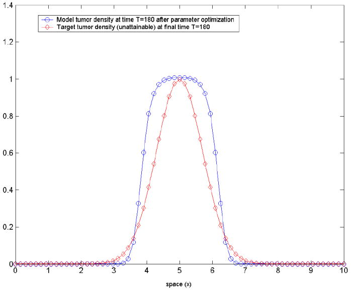
the model-predicted tumor density corresponding to the optimized set of parameters (ρ, p₁, p₂) and the (a priori unattainable) target tumor density c* (x, T) given by equation (31) at the final moment of time t = T. This is the closest the tumor density generated by model can get to the prescribed Gaussian profile.

Figure 3. Test-case 2.

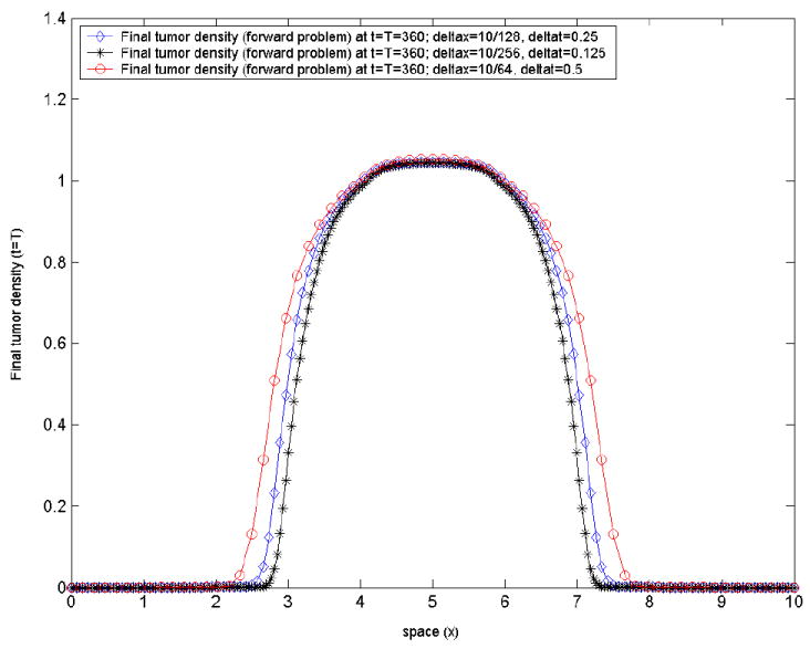
the model-generated tumor density at final time t = T, corresponding to the prescribed model parameters(ρ, p₁, p₂) = (0.05, 1.2, 0.1), by varying the mesh size and the time-step. We illustrate the stable behavior of the forward problem numerical solution with mesh/time-step refinement.

Table 2.

Test-case 2: optimization results summary. Three optimization parameters: (ρ, p₁, p₂). The optimization problem is solved in three different ways, with the corresponding converged solution shown. The original parameter values (ρ, p₁, p₂) = (0.05, 1.2, 0.1) very closely retrieved. As in test-case 1 before, the two gradient-based methods here show similar performance, about 2.5 times faster than a direct search.

	ρ	p1	p2	Relative run time
Direct search	0.0500	1.1999	0.0999	1
FD gradient-based	0.0499	1.1980	0.0994	0.41
Adjoint gradient-based	0.0500	1.2018	0.1004	0.43

Figure 4. Test-case 3.

the initial landmark position (top) and the corresponding model-generated target landmarks (bottom) at final time t = T for (ρ, p₁, p₂) = (0.05, 1.2, 0.1). Initial landmarks picked to sample different spatial areas of interest: close to the initial tumor boundary, close to the ‘brain’ boundary, and in-between.

Table 3.

Optimization results for test-case 3, with the objective functional based on landmarks. Three optimization parameters: (ρ, p₁, p₂). Optimization problem solved in three different ways, with the corresponding converged solution shown. The original parameter value ρ = 0.05 very closely retrieved, while the other two parameters (p₁, p₂) not so closely matched. In this particular case, for the adjoint gradient-based method, a trust-region search performed better than a line-search in terms of recovering the target landmarks within the specified tolerance, but slower.

	ρ	p1	p2	Relative run time
Direct search	0.0481	0.938	0.0191	1
FD gradient-based	0.0480	0.8913	0.0106	0.2
Adjoint gradient-based	0.0478	0.9133	0.0232	0.5

Figure 5. Test-case 3.

Top: landmark position; the initial and target landmark position marked with circles. Landmarks displacement illustrates the nonlinear coupling between tumor growth and subsequent mechanical deformations (mass-effect) in our model. Bottom: the final (time t = T) tumor density profile.

Table 4.

Optimization results for test-case 4. Six optimization parameters: (ρ, p₁, p₂, c₁, c₂, c₃). Optimization problem solved in three different ways, with the corresponding converged solution shown. The original parameter values (ρ, p₁, p₂, c₁, c₂, c₃) = (0.05, 1.2, 0.1, 0.0004, 5, 0.06) closely retrieved by the gradient-based methods, not so well by the direct search. The adjoint-based method exhibits best scalability with respect to the number of inversion variables (see also table 5). Number of iterations: 486 for the direct search, 67 for the FD gradient-based and 57 for the adjoint gradient-based.

	ρ	p1	p2	c1	c2	c3	Relative run time
Direct search	0.0535	0.9819	0.006	0.00053	4.9994	0.0132	1
FD gradient-based	0.0500	1.1700	0.0920	0.000398	4.9997	0.0596	0.52
Adjoint gradient-based	0.0498	1.1689	0.0903	0.000412	4.9998	0.0593	0.21

Table 5.

Optimization results for test-case 4, with only three optimization parameters: (ρ, p₁, p₂); (c₁, c₂, c₃) = (0.0004, 5, 0.06) kept fixed. Optimization problem solved in three different ways, with the corresponding converged solution shown. The original parameter values (ρ, p₁, p₂) = (0.05, 1.2, 0.1) reasonably retrieved by all three methods.

	ρ	p1	p2	Relative run time
Direct search	0.0499	1.1670	0.0916	1
FD gradient-based	0.0499	1.1441	0.0854	0.37
Adjoint gradient-based	0.0499	1.1015	0.0744	0.25

Figure 7.

Optimization results for test-case 5. Initial target density closely recaptured.

6 Illustration of simulations on real brain tumor patient MR images

We include this last section here for the purpose of highlighting the potential of the proposed model to capture well real brain patient data. Applying the overall methodology proposed in this paper to real brain tumor patient MR images is on-going work [22].

The simulations illustrated here are for a human brain tumor patient, with low-grade glioma progressing into higher malignancy. Two T1 MRI scans with approximately 2.5 years in-between were available. 21 pairs of corresponding landmark points were manually identified by an expert human rater in the starting (original scan, when patient first diagnosed with low-grade glioma) and target (correspondingly aligned scan 2.5 years later) 3D MR images. Segmentation of the images in this case included only white matter and ventricles, for which we assumed fixed elastic properties (stiffness and compressibility, respectively) E_white = 2.1KPa, E_ventricles = 500Pa, ν_white = 0.45, ν_ventricles = 0.1 [17, 22].

Given model-generated landmarks and manually-tracked landmarks, we seek to find a deformation that minimizes the mismatch between the predicted and the actual deformation (see Figure 8).

Figure 8. Illustration of Landmark Registration.

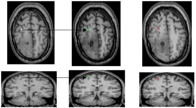
Illustration of the landmark placement/registration in two serial scans of a human subject with progressive low grade glioma that are approximately 2.5 years apart. From left to right: the first column displays two landmarks manually placed by an expert in the early scan; the second column shows the two landmarks manually tracked by the same expert in the later scan. Finally, the third column shows the corresponding model-generated landmarks, for a given choice of the model parameters.

We estimated an approximate initial tumor location (center and size) from the early scan and inverted for four parameters only: initial tumor density magnitude, tumor cell diffusivity in white matter, tumor growth rate and tumor mass-effect strength (parameter p₁ in equation 10). The results, illustrating the behavior of our model with optimized parameters, are depicted in figure 9. Guided by the deformation of only 21 pairs of landmarks, the model appears able to capture reasonably the tumor behavior in the actual patient. This is particularly visible in the axial slice (figure 9 - top), in the ventricle compression - relatively similar in the actual patient image and the model-generated image. In the sagittal view (figure 9 - bottom), the deformation of the corpus calosum produced by the growing tumor in the actual patient image is visibly similar to the model-generated one.

Figure 9. Real brain tumor images, human subject.

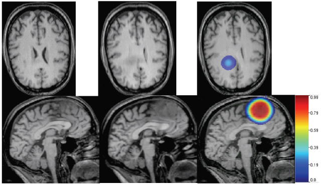
Left to right: starting scan, T1 MR; target scan, T1 MR; simulated tumor growth and mass effect via our model: tumor color maps overlaid on the model-deformed image, with corresponding color bar attached. Reasonable visual agreement observed between the actual patient target image (second column) and the simulated one (third column, right), guided by only 21 pairs of corresponding landmarks manually placed by a human rater in the early scan and the late (target) scan, respectively. Note that in this case, the brain was segmented into white matter and ventricles only, which explains the quasi-uniform tumor growth pattern.

For such preliminary assessment of the model behavior on real brain tumor patient data, we have used APPSPACK, an optimization library from the Sandia National Laboratories [40, 41, 42]. The forward problem in this case was numerically solved using a spatial discretization with 65³ nodes and five equal time steps.

The optimization variables should lie within a physiological range. Their precise range, however, is unknown. For example, the reaction term in our tumor model is a crude approximation of tumor growth. Second, even if the model were correct, there would be significant inter-individual variability. We used guiding values from existing literature for the tumor cell diffusivity in white and grey matter [10], but we had to use numerical experiments to determine reasonable ranges for ρ and p₁.

The results of our optimization experiments support an optimization method with the gradient of the objective functional estimated in terms of the adjoint variables, which is efficient and scales well with the number of inversion variables (design parameters), unlike a direct search method. Regarding an optimization method with the approximation of the gradient via finite differences (FD), it is generally comparable with an adjoint-based method for a relatively small number of design parameters (e.g., one to three/four parameters to be estimated)¹⁰ However, when the number of design variables is increased (e.g., to six or more), an adjoint-based optimization method remains most efficient. Within our proposed framework, it is of fundamental importance to design an optimization procedure that allows flexibility in introducing additional unknown parameters to be estimated (e.g., material properties, more complex tumor growth models).

7 Discussion and conclusions

A variety of mathematical models for the spatio-temporal evolution of solid tumors have been developed over the past three decades [7]. These models involve a number of unknown parameters that are typically very difficult to estimate in-vivo via existing experimental and imaging set-ups. One way around this problem is inverse estimation, i.e., based on data from a patient, find the best set of parameters of a tumor growth model that fits the patient’s data (e.g. images). Complex models, however, involve a large number of unknown parameters. This makes complex models difficult to calibrate in clinical setting due to limited number of images that capture the tumor time evolution. ¹¹

In this article we focused on models with a number of parameters that could be realistically determined and validated from existing data, via inverse estimation. The key aspects that we are interested in capturing are: spatio-temporal spread of gliomas and mechanical deformations from tumor growth.

We proposed an Eulerian framework for modeling gliomas growth and the subsequent mechanical impact on the surrounding brain tissue (mass-effect), with estimation of unknown parameters via PDE-constrained optimization. To our knowledge, this is the first attempt to introduce an adjoint-based, PDE-constrained optimization formulation in the context of modeling spatio-temporal tumor evolution. We introduced numerical schemes for the solution of the systems of nonlinear PDEs governing the forward, adjoint, and inverse problems. The numerical solution procedure is being successfully applied on 3D images of brain tumor subjects. The criteria in designing the numerical schemes, were computational cost and robustness.

Through a series of 1D experiments, which are better suited for analysis, comparison and proof-of-concept, we showed the advantage of estimating the gradient of the objective functional in terms of the adjoints for solving the optimization problems. Evaluating the gradient through adjoints requires one solve of the adjoint system (per optimization iteration) regardless of the number of inversion variables. This provides excellent scalability with respect to the number of control variables.

Effects of treatment (chemotherapy, radiotherapy) and recurrence of gliomas after resection [23], can be incorporated in the current framework. Tumor model parameter estimation via PDE-constrained optimization, is general and not necessarily restricted to medical imaging data. Imaging data contains readily available patient-specific information that has not been exploited so far for calibrating and validating mathematical models of tumor growth. The present paper was dedicated to formulation and methods. Numerical experiments have been presented, for a preliminary evaluation of the overall formulation/methodology. The benefits of the adjoint-based optimization methods in terms of scalability with the number of control variables have been highlighted through a series of test-cases. We are currently working on the full 3D MRI-based simulations [22].

Figure 6. Test-case 4.

Top: the initial tumor ‘seed’, assumed of the form (32); in this optimization experiment, c₁, c₂, c₃ (location and size of the seed) are part of the inversion parameter set. Bottom: corresponding spatial tumor evolution at later times. Close match is retrieved via the adjoint-based optimization.

APPENDIX

A. The Karush-Kuhn-Tucker Optimality conditions

The first-order necessary optimality conditions for optimality, or KKT conditions, may be derived by introducing an associated Lagrangian functional:

$$L_1({\varphi }_1,{\mathit{\zeta }}_1,{\mathit{g}}_1)=J_1+\frac{a}{2}({\rho }^2+p_1^2+p_2^2)+{\mathit{\int }}_U\alpha (\frac{\partial c}{\partial t}-\nabla \cdot (D\nabla c)+\nabla \cdot (c\mathbf{v})-\rho c(1-c))d\mathbf{x}dt+{\mathit{\int }}_U\mathit{\beta }\cdot (\nabla \cdot ((\lambda \nabla \cdot \mathbf{u})+\mu (\nabla \mathbf{u}+\nabla {\mathbf{u}}^T))-p_1{e}^{-\frac{p_2}{c^s}}{e}^{-\frac{p_2}{{(2-c)}^s}}\nabla c)d\mathbf{x}dt+{\mathit{\int }}_U\mathit{\xi }\cdot (\mathbf{v}-\frac{\partial \mathbf{u}}{\partial t})d\mathbf{x}dt+{\mathit{\int }}_{\mathrm{U}}{\gamma }_D(\frac{\partial D}{\partial t}+\nabla D\cdot \mathbf{v})d\mathbf{x}dt+{\mathit{\int }}_U{\gamma }_{\lambda }(\frac{\partial \lambda }{\partial t}+\nabla \lambda \cdot \mathbf{v})d\mathbf{x}dt+{\mathit{\int }}_U{\gamma }_{\mu }(\frac{\partial \mu }{\partial t}+\nabla \mu \cdot \mathbf{v})d\mathbf{x}dt,$$ (A-1)

where the variables ζ₁ = (α, β, ξ, γ_D, γ_λ, γ_μ) represent the adjoint (dual) variables of the corresponding state variables ϕ₁ = (c, u, v, D, λ, μ) and g₁ = (ρ, p₁, p₂) are the inversion variables.

By requiring stationarity of the Lagrangian functional with respect to the adjoint variables, to the states, and to the inversion parameters respectively, the KKT optimality conditions in this case are obtained, consisting of the forward problem defined by equations (11)-(21). The adjoint equations

$$\begin{array}{r}-\frac{\partial \alpha }{\partial t}-\nabla \cdot (D\nabla \alpha )-\mathbf{v}\cdot \nabla \alpha -\alpha \rho (1-2c)+f(c,p_1,p_2)\nabla \cdot \mathit{\beta }+\\ \sum _{k=1}^N\delta (t-t_k)(c-c_k^{\ast })=0\mathrm{in}U\\ \alpha (\mathbf{x},t=T)=0\mathrm{in}\omega \\ \frac{\partial \alpha }{\partial n}=0\mathrm{on}\partial \omega \times (0,T).\end{array}$$ (A-2)

$$\begin{array}{r}\nabla \cdot ((\lambda \nabla \cdot \mathit{\beta })+\mu (\nabla \mathit{\beta }+\nabla {\mathit{\beta }}^T))+\frac{\partial \mathit{\xi }}{\partial t}=0\mathrm{in}U\\ \beta =0\mathrm{on}\partial \omega \times (0,T)\\ \mathit{\xi }(\mathbf{x},t=T)=0\mathrm{in}\omega \\ \beta (\mathbf{x},t=T)=0\mathrm{in}\omega .\end{array}$$ (A-3)

$$-c\nabla \alpha +{\gamma }_D\nabla D+{\gamma }_{\lambda }\nabla \lambda +{\gamma }_{\mu }\nabla \mu +\mathit{\xi }=0\mathrm{in}U.$$ (A-4)

$$\begin{array}{r}-\frac{\partial {\gamma }_D}{\partial t}-\nabla \cdot ({\gamma }_D\mathbf{v})+\nabla c\cdot \nabla \alpha =0\mathrm{in}U\\ -\frac{\partial {\gamma }_{\lambda }}{\partial t}-\nabla \cdot ({\gamma }_{\lambda }\mathbf{v})-(\nabla \cdot \mathbf{u})\mathbf{I}\cdot \nabla \mathit{\beta }=0\mathrm{in}U\\ -\frac{\partial {\gamma }_{\mu }}{\partial t}-\nabla \cdot ({\gamma }_{\mu }\mathbf{v})-(\nabla \mathbf{u}+\nabla {\mathbf{u}}^T)\cdot \nabla \mathit{\beta }=0\mathrm{in}U\\ {\gamma }_D(\mathbf{x},t=T)=0\mathrm{in}\omega \\ {\gamma }_{\lambda }(\mathbf{x},t=T)=0\mathrm{in}\omega \\ {\gamma }_{\mu }(\mathbf{x},t=T)=0\mathrm{in}\omega .\end{array}$$ (A-5)

And the inversion equations:

$$\begin{array}{r}a\rho -{\mathit{\int }}_U\alpha c(1-c)d\mathbf{x}dt=0\\ a{p}_1+{\mathit{\int }}_U\mathit{\beta }\cdot (\frac{\partial f}{\partial p_1})\nabla cd\mathbf{x}dt=0\\ a{p}_2+{\mathit{\int }}_U\mathit{\beta }\cdot (\frac{\partial f}{\partial p_2})\nabla cd\mathbf{x}dt=0.\end{array}$$ (A-6)

In the case of a landmark-based functional we only have a few changes: The forward problem consists of (11)-(21) plus equation (24); The adjoint equations consist of (A-4), (A-5), and the following reduced version of (A-2)

$$\begin{array}{r}-\frac{\partial \alpha }{\partial t}-\nabla \cdot (D\nabla \alpha )-\mathbf{v}\cdot \nabla \alpha -\alpha \rho (1-2c)+f(c,p_1,p_2)\nabla \cdot \mathit{\beta }=0\mathrm{in}U\\ \alpha (\mathbf{x},t=T)=0\mathrm{in}\omega \\ \frac{\partial \alpha }{\partial n}=0\mathrm{on}\partial \omega \times (0,T),\end{array}$$ (A-7)

an augmented version of (A-4) given by

$$-c\nabla \alpha +{\gamma }_D\nabla D+{\gamma }_{\lambda }\nabla \lambda +{\gamma }_{\mu }\nabla \mu +{\gamma }_{\psi }\nabla \psi +\mathit{\xi }=0\mathrm{in}U,$$ (A-8)

plus an additional equation for the newly introduced adjoint variable γ_ψ

$$\begin{array}{r}-\frac{\partial {\gamma }_{\psi }}{\partial t}-\nabla \cdot ({\gamma }_{\psi }\mathbf{v})+\sum _{k=1}^N\sum _{l=1}^L\delta (t-t_k)\delta (\mathbf{x}-{\mathbf{x}}_l^k)(\psi (\mathbf{x},t)-{\mathbf{x}}_l)=0\mathrm{in}U\\ {\gamma }_{\psi }(\mathbf{x},t=T)=0\mathrm{in}\omega ;\end{array}$$ (A-9)

the inversion equations remain the same.

B. The fictitious domain method

In the fictitious domain method, the target domain ω is embedded on a larger computational rectangular domain (box) - let it be denoted by Ω from here on. The PDEs originally defined on ω must be appropriately extended to Ω, such that the true boundary conditions prescribed on ∂ω are approximated [17]. In our case, both in the forward problem (equations (11)-(21)) and the adjoint one (e.g. equations (A-2)-(A-5)), we only have to deal with homogeneous Neumann/Dirichlet boundary conditions on ∂ω, which makes extension to Ω straight-forward. Thus, let us introduce the following definitions:

$$D_{\mathit{\epsilon }}=\{\begin{array}{ll}D,& \mathrm{in}\omega \\ \mathit{\epsilon }D,& \mathrm{in}\mathrm{\Omega }\backslash \overline{\omega }\end{array}$$ (B-1)

$${(\lambda ,\mu )}_{\mathit{\epsilon }}=\{\begin{array}{cc}(\lambda ,\mu ),& \mathrm{in}\omega \hfill \\ \frac{1}{\mathit{\epsilon }}(\lambda ,\mu ),& \mathrm{in}\mathrm{\Omega }\backslash \overline{\omega }\hfill \end{array}$$ (B-2)

where ε > 0 is a ‘small’ positive number, regarded as a penalty parameter. Then the forward diffusion equation (11) on ω is being replaced by its extension to Ω, with D replaced by D_ε and v = 0, ρ = 0 in Ω\ ω̄. The zero flux boundary condition (16) is now imposed on ∂Ω. The forward elasticity equation (12) on ω is being replaced by its extension to Ω, with (λ, μ) replaced by (λ, μ)_ε and f ≡ 0 in Ω\ ω̄. The zero displacement boundary condition (17) is re-imposed on ∂Ω. Similar extensions can be employed for the adjoint equations (e.g. equations (A-2)-(A-5) in Appendix). In the end, both the forward problem and the adjoint problem can be equivalently replaced by their extensions on the regular domain Ω (where the actual numerical discretization in space shall be performed). It is expected [43] that a weak solution exists to each problem, which is smooth on ω and Ω\ ω̄ respectively, and satisfies the actual boundary conditions on ∂ω in the limit ε → 0. The expected order of convergence is at least $O(\sqrt{\mathit{\epsilon }})$ (in H¹) [44].

C. Numerical solution procedure for the adjoint equations

The adjoint problem is given by (A-2)-(A-5) with ζ = (c, u, v, D, λ, μ) known. Let ζ_adj = (α, β, ξ, γ_D, γ_λ, γ_μ) denote the vector of adjoint variables. By change of variables $\tau =T-t,\frac{\partial }{\partial t}=-\frac{\partial }{\partial \tau },0\le \tau \le T$ and the terminal conditions at t = T become initial conditions. If ${\mathit{\zeta }}_{\mathit{adj}}^n=(\alpha ,\mathit{\beta },\mathit{\xi },{\gamma }_D,{\gamma }_{\lambda },{\gamma }_{\mu })$ is the solution at time τ = τ_n, then a simple way to update the solution ${\mathit{\zeta }}_{\mathit{adj}}^{n+1}$ at the next time step τ_n+1 = τ_n + Δt is as follows:

1. Solve the adjoint diffusion equation (A-2) using a fractional step method:

   1. Solve $\frac{\partial \alpha }{\partial t}=A_2(\alpha ,\mathbf{v})$ over time Δt with data (αⁿ, vⁿ), using an explicit upwind scheme, to obtain α*;
   2. Solve $\frac{\partial \alpha }{\partial t}=\mathrm{\Delta }(\alpha ,D)$ over time Δt with data (α*, Dⁿ⁺¹), using an implicit scheme, to obtain α**;
   3. Solve $\frac{\partial \alpha }{\partial t}=R_1(\alpha )+R_2(\beta ,c)$ over time Δt with data α** to obtain αⁿ⁺¹. The reaction term R₁(α) = αρ(1 − 2c) is treated implicitly in time, while the term containing β is treated explicitly.

2. Solve the adjoint material advection equations (A-5) using an explicit conservative upwind scheme over time Δt to obtain $({\gamma }_D^{n+1},{\gamma }_{\lambda }^{n+1},{\gamma }_{\mu }^{n+1})$.

3. Solve the velocity adjoint equation (A-4) - algebraic equation in the adjoint unknown ξ - to update ξⁿ⁺¹.

4. Solve the adjoint elasticity equation (A-3) with data (ξⁿ⁺¹, λⁿ⁺¹, μⁿ⁺¹) to obtain βⁿ⁺¹.

D. A convergence study against synthetic closed-form solutions

Consider the simplified case of a homogeneous material: D_w = D_g = D and m_w = m_g = m. For the 1D forward problem, let us introduce the following expressions:

$$c_{\mathit{an}}(x,t)=\frac{t}{T}+e^{-A^2\mathit{Dt}}{c}_0(\mathit{cos}(\mathit{Ax}+B)+1),x\in \left[x_1,x_2\right],t\in \left[0,T\right]$$ (D-1)

$$u_{\mathit{an}}(x,t)=\frac{1}{L}{(\frac{t}{T})}^2(x-x_1)(x-x_2)\mathit{sin}(\mathit{Ax}+B),x\in \left[x_1,x_2\right],t\in \left[0,T\right]$$ (D-2)

$$v_{\mathit{an}}(x,t)=2\frac{1}{L}\frac{t}{T^2}(x-x_1)(x-x_2)\mathit{sin}(Ax+B),x\in \left[x_1,x_2\right],t\in \left[0,T\right],$$ (D-3)

where $A=\frac{\pi }{x_2-x_1}$ and $B=-\frac{\pi x_1}{x_2-x_1}$ are constants such that c_an, u_an and v_an satisfy the prescribed initial and boundary conditions (16)-(20). L is a length scaling factor, e.g., the length of the space interval and c₀ is a positive constant. We refer to these as ‘synthetic closed-form solutions’ for the 1D forward problem. If we plug these expressions into the 1D version of equation (11) and equation (29), we obtain the corresponding PDEs for c_an and u_an, similar to the original equations with properly modified source/force terms.

Similarly, for the 1D adjoint problem, we introduce

$${\alpha }_{\mathit{an}}(x,t)=(\frac{e^{-A^2\mathit{Dt}}-e^{-A^2\mathit{DT}}}{1-e^{-A^2\mathit{DT}}}){\alpha }_0\mathit{cos}(Ax+B),x\in \left[x_1,x_2\right],t\in \left[0,T\right]$$ (D-4)

$${\beta }_{\mathit{an}}(x,t)={(\frac{t-T}{T})}^2{\beta }_0{\mathit{sin}}^2(\mathit{Ax}+B),x\in \left[x_1,x_2\right],t\in \left[0,T\right],$$ (D-5)

$${\xi }_{\mathit{an}}=c_{\mathit{an}}(x,t)\frac{\partial {\alpha }_{\mathit{an}}}{\partial x},x\in \left[x_1,x_2\right],t\in \left[0,T\right],$$ (D-6)

where α₀ and β₀ are corresponding scaling factors. Note that the above expressions for α_an and β_an do satisfy both the boundary and terminal conditions at t = T prescribed in the adjoint problem for the adjoint variables α and β. Also ξ_an satisfies the prescribed terminal condition at t = T for the adjoint variable ξ. As before, these are referred to as ‘synthetic closed-form solutions’ for the 1D adjoint problem. If we plug these expressions into the 1D versions of equations (A-2) and (A-3), we obtain the corresponding PDEs for α_an and β_an.

We applied the proposed numerical solution procedure for both the forward and the adjoint problems and compared the errors of the numerical solutions against the synthetic closed-form solutions during mesh refinement. Results are summarized in tables 6 and 7: no fictitious domain and a fictitious domain approach, respectively. In both cases, the results shown here correspond to the following choice of parameter values: x₁ = 2, x₂ = 8, T = 1; D = 0.0001, ρ = 0.01, m = 1, p₁ = 1, p₂ = 0.1; c₀ = 0.05, L = 6, α₀ = 1, β₀ = 1. In the first case, with no fictitious domain, the physical spatial domain [2, 8] is discretized using an uniform mesh, of size Δx. The time interval [0, T] is also discretized uniformly, with time-step Δt. The corresponding relative ∥∥_∞ errors $({\Vert {\mathit{sol}}_{\mathit{an}}\Vert }_{\mathrm{\infty }}^{\mathit{rel}}=\frac{{\Vert {\mathit{sol}}_{\mathit{an}}^{\mathit{numeric}}-{\mathit{sol}}_{\mathit{an}}\Vert }_{\mathrm{\infty }}}{{\Vert {\mathit{sol}}_{\mathit{an}}\Vert }_{\mathrm{\infty }}})$ with respect to the synthetic closed-form solutions at time $t=\frac{T}{2}$ are shown in table 6. The results verify the first-order convergence rate. In the second case, we test a fictitious domain approach, where the physical spatial domain [2, 8] is embedded on a larger (fictitious) domain - here chosen [0, 10]. This whole larger domain is now discretized using an uniform mesh, of size Δx. A contrast factor ε = (Δx)² is used between the material properties inside the real domain [2, 8] and outside, in the fictitious domain [0, 2) ∪ (8, 10]. The time interval [0, T] is discretized uniformly, as before, with time-step Δt. The corresponding relative ∥∥_∞ errors with respect to the synthetic closed-form solutions at time $t=\frac{T}{2}$ are shown in table 7. Our fictitious domain implementation in this case retains the overall first-order accuracy, with errors comparable to the implementation without fictitious domain.

Table 6.

Convergence study, no fictitious domain. The relative ∥∥_∞ error of the numerical solution with respect to the synthetic closed-form solution at time $t=\frac{T}{2}$ shown.

	${\Vert c_{\mathit{an}}\Vert }_{\mathrm{\infty }}^{\mathit{rel}}$	${\Vert u_{\mathit{an}}\Vert }_{\mathrm{\infty }}^{\mathit{rel}}$	${\Vert {\alpha }_{\mathit{an}}\Vert }_{\mathrm{\infty }}^{\mathit{rel}}$	${\Vert {\beta }_{\mathit{an}}\Vert }_{\mathrm{\infty }}^{\mathit{rel}}$
Δx = 8/64, Δt = 0.01	0.001148	0.003600	0.005842	0.030570
Δx = 8/128, Δt = 0.005	0.000556	0.001543	0.002995	0.015267
Δx = 8/256, Δt = 0.0025	0.000275	0.000706	0.001516	0.007629
Δx = 8/512, Δt = 0.000625	0.000137	0.000336	0.000763	0.003813

Table 7.

Convergence study for a fictitious domain approach. The relative ∥∥_∞ error of the numerical solution with respect to the synthetic closed-form solution at time $t=\frac{T}{2}$ shown.

	${\Vert c_{\mathit{an}}\Vert }_{\mathrm{\infty }}^{\mathit{rel}}$	${\Vert u_{\mathit{an}}\Vert }_{\mathrm{\infty }}^{\mathit{rel}}$	${\Vert {\alpha }_{\mathit{an}}\Vert }_{\mathrm{\infty }}^{\mathit{rel}}$	${\Vert {\beta }_{\mathit{an}}\Vert }_{\mathrm{\infty }}^{\mathit{rel}}$
Δx = 10/64, Δt = 0.01	0.003651	0.003651	0.007040	0.018795
Δx = 10/128, Δt = 0.005	0.000708	0.001818	0.003540	0.009070
Δx = 10/256, Δt = 0.0025	0.000344	0.000951	0.001771	0.005512
Δx = 10/512, Δt = 0.000625	0.000168	0.000407	0.000899	0.002404

References

- 1.Alvord JE, Shaw C. Neoplasms affecting the nervous system of the elderly. In: Duckett S, editor. The Pathology of the Aging Human Nervous System. 2002. [Google Scholar]
- 2.Bernstein J, Goldberg W, Laws EJ. Human malignant astrocytoma xenografts migrate in rat brains: a model for central nervous system cancer research. Journal of Neuroscience Research. 1989;22:134–143. doi: 10.1002/jnr.490220205. [DOI] [PubMed] [Google Scholar]
- 3.Chicoine MR, Silbergeld DL. Assessment of brain tumor cell motility in vivo and in vitro. Journal of Neurosurgery. 1995;82:615–622. doi: 10.3171/jns.1995.82.4.0615. [DOI] [PubMed] [Google Scholar]
- 4.Geer CP, Grossman SA. Interstitial fluid flow along white matter tracts: A potentially important mechanism for the dissemination of primary brain tumors. Journal of Neuro-oncology. 1997;32:193–201. doi: 10.1023/a:1005761031077. [DOI] [PubMed] [Google Scholar]
- 5.Kansal AR, Torquato S, et al. Simulated brain tumor growth dynamics using a three-dimensional cellular automaton. Journal of theoretical biology. 2000;203:367–382. doi: 10.1006/jtbi.2000.2000. [DOI] [PubMed] [Google Scholar]
- 6.Mansury Y, Deisboeck TS. Simulating ‘structure-function’ patterns of malignant brain tumors. Physica A: Statistical Mechanics and its Applications. 2004;331:219–232. [Google Scholar]
- 7.Araujo RP, McElwain DLS. A history of the study of tumor growth: The contribution of mathematical modeling. Bulletin of Mathematical Biology. 2004;66:1039–1091. doi: 10.1016/j.bulm.2003.11.002. [DOI] [PubMed] [Google Scholar]
- 8.Alarcon T, Byrne HM, Maini P. A multiple scale model for tumor growth. Multiscale Modeling and Simulation. 2005;3:440–475. [Google Scholar]
- 9.Chaplain MAJ, Anderson ARA. Mathematical modelling of tissue invasion. In: Preziosi L, editor. Cancer modeling and simulation. 2003. [Google Scholar]
- 10.Swanson KR, Alvord EC, Murray JD. A quantitative model for differential motility of gliomas in grey and white matter. Cell Proliferation. 2000;33:317–329. doi: 10.1046/j.1365-2184.2000.00177.x. [DOI] [PMC free article] [PubMed] [Google Scholar]
- 11.Tracqui P, Mendjeli M. Modelling three-dimensional growth of brain tumors from time series of scans. Mathematical Models and Methods in Applied Sciences. 1999;9:581–598. [Google Scholar]
- 12.Habib S, Molina-Paris C, Deisboeck T. Complex dynamics of tumors: modling an emerging brain tumor system with coupled reaction-diffusion equations. Physica A: Statistical Mechanics and its Applications. 2003;327:501–524. [Google Scholar]
- 13.Byrne HM, King JR, McElwain DLS, Preziosi L. A two-phase model of solid tumor growth. Applied Mathematics Letters. 2002;16:567–573. [Google Scholar]
- 14.Araujo RP, McElwain DLS. A mixture theory for the genesis of residual stresses in growing tissues i: A general formulation. Journal on Applied Mathematics. 2005;65:1261–1284. [Google Scholar]
- 15.Wasserman RM, Acharya RS, Sibata C, Shin KH. Patient-specific tumor prognosis prediction via multimodality imaging. Proc SPIE Int Soc Opt Eng. 1996;2709 [Google Scholar]
- 16.Kyriacou S, Davatzikos C, et al. Nonlinear elastic registration of brain images with tumor pathology using a biomechanical model. IEEE Transactions on Medical Imaging. 1999;18:580–592. doi: 10.1109/42.790458. [DOI] [PubMed] [Google Scholar]
- 17.Hogea C, Abraham F, Biros G, Davatzikos C. Fast solvers for soft tissue simulation with application to construction of brain tumor atlases. IEEE Transactions on Medical Imaging. 2006 [Google Scholar]
- 18.Kyriacou S, Davatzikos C. A biomechanical model of soft tissue deformation, with applications to non-rigid registration of brain images with tumor pathology. LNCS. 1998;1496:531–5538. [Google Scholar]
- 19.Mohamed A, Davatzikos C. Proceedings of Medical Image Computing and Computer-Assisted Intervention. Palm Springs: 2005. Finite element modeling of brain tumor mass-effect from 3d medical images. [DOI] [PubMed] [Google Scholar]
- 20.Clatz O, Sermesant M, Bondiau PY, Delingette H, Warfield SK, Malandain G, Ayache N. Realistic simulation of the 3d growth of brain tumors in mr images coupling diffusion with mass effect. IEEE Trans on Med Imaging. 2005;24:1334–1346. doi: 10.1109/TMI.2005.857217. [DOI] [PMC free article] [PubMed] [Google Scholar]
- 21.Zacharaki E, Hogea C, Biros G, Davatzikos C. Biomechanical simulations in deformable registration of brain tumor images. IEEE Transactions on Biomedical Engineering to appear. 2007 doi: 10.1109/TBME.2007.905484. [DOI] [PMC free article] [PubMed] [Google Scholar]
- 22.Hogea C, Biros G, Davatzikos C. Proceedings of MICCAI. Brisbane, Australia: 2007. Glioma growth and mass effect in 3d images. [DOI] [PubMed] [Google Scholar]
- 23.Swanson KR, Bridge C, Murray JD, Alvord EC. Virtual and real brain tumors: using mathematical modeling to quantify glioma growth and invasion. Journal of the Neurological Sciences. 2003;216:1–10. doi: 10.1016/j.jns.2003.06.001. [DOI] [PubMed] [Google Scholar]
- 24.Giese A, Westphal M. Glioma invasion in the central nervous system. Neurosurgery. 1996;39:235–250. doi: 10.1097/00006123-199608000-00001. [DOI] [PubMed] [Google Scholar]
- 25.Hogea C. PhD thesis. Binghamton University; 2005. Modeling Tumor Growth: a Computational Approach in a Continuum Framework. [Google Scholar]
- 26.Hagemann A, Rohr K, et al. Biomechanical modeling of the human head for physically based, nonrigid image registration. IEEE Transactions on Medical Imaging. 1999;18:875–884. doi: 10.1109/42.811267. [DOI] [PubMed] [Google Scholar]
- 27.Zacharaki E, Shen D, Mohamed A, Davatzikos C. Registration of brain images with tumors: Towards the construction of statistical atlases for therapy planning. Biomedical Imaging: Macro to Nano, 2006. 3rd IEEE International Symposium on; 2006. pp. 197–200. [Google Scholar]
- 28.Mandonnet E, Delattre J, et al. Continuous growth of mean tumor diameter in a subset of grade ii gliomas. ANNALS OF NEUROLOGY. 2003;53:524–528. doi: 10.1002/ana.10528. [DOI] [PubMed] [Google Scholar]
- 29.Poptani H, Puumalainen A, et al. Monitoring thymidine kinase and ganciclovir-induced changes in rat malignant glioma in vivo by nuclear magnetic resonance imaging. CANCER GENE THERAPY. 1998;5:101–109. [PubMed] [Google Scholar]
- 30.Verma R, Ou Y, Lee S, Melhem E, Davatzikos C. Integration of multiple magnetic resonance images via pattern recognition. Radiology. 2005 Submitted. [Google Scholar]
- 31.Gunzburger M. Perspectives in Flow Control and Optimization. SIAM; 2002. [Google Scholar]
- 32.Nocedal J, Wright SJ. Numerical Optimization. Springer; 1999. [Google Scholar]
- 33.Kress R. Applied Mathematical Sciences. Springer; 1999. Linear Integral Equations. [Google Scholar]
- 34.Hogea C, Abraham F, Biros G, Davatzikos C. Medical Image Computing and Computer-Assisted Intervention Workshop on Biomechanics. Copenhagen: 2006. A framework for soft tissue simulations with applications to modeling brain tumor mass-effect in 3d images. [Google Scholar]
- 35.Tyson R, Stern L, LeVeque R. Fractional step methods applied to a chemotaxis model. J Math Biol. 2000;41:455–475. doi: 10.1007/s002850000038. [DOI] [PubMed] [Google Scholar]
- 36.Verwer J, Hundsdorfer W, Blom J. Report MAS-R9825. CWI; Amsterdam: 1991. Numerical time integration for air pollution models. [Google Scholar]
- 37.Osher S, Fedkiw R. Level Set Methods and Dynamic Implicit Surfaces. Springer; 2003. [Google Scholar]
- 38.LeVeque R. Numerical Methods for Conservation Laws. Birkhauser; 1992. [Google Scholar]
- 39.Akcelik V, Biros G, Draganescu A, Ghattas O, Hill J, Bloemen BV. Dynamic data-driven inversion for terascale simulations: real-time identification of airborne contaminants. ACM/IEEE SCXY conference series. 2005 [Google Scholar]
- 40.Kolda T, et al. APPSPACK home page. 2005 http://software.sandia.gov/appspack/version5.0.
- 41.Gray GA, Kolda TG. Algorithm 8xx: APPSPACK 4.0: Asynchronous parallel pattern search for derivative-free optimization. ACM Transactions on Mathematical Software. 2005 To appear (Accepted Nov. 2005) [Google Scholar]
- 42.Kolda TG. Revisiting asynchronous parallel pattern search for nonlinear optimization. SIAM Journal on Optimization. 2005;16:563–586. [Google Scholar]
- 43.Zhu S, Yuan G, Sun W. Convergence and stability of explicit/implicit schemes for parabolic equations with discontinuous coefficients. International Journal of Numerical Analysis and Modeling. 2004;1:131–145. [Google Scholar]
- 44.DelPino S, Pironneau O. Numerical Methods for Scientific Computing Variational Problems and Applications. Barcelona: 2003. A fictitious domain based general pde solver. [Google Scholar]