The construction of next-generation matrices for compartmental epidemic models

Abstract

The basic reproduction number ℛ₀ is arguably the most important quantity in infectious disease epidemiology. The next-generation matrix (NGM) is the natural basis for the definition and calculation of ℛ₀ where finitely many different categories of individuals are recognized. We clear up confusion that has been around in the literature concerning the construction of this matrix, specifically for the most frequently used so-called compartmental models. We present a detailed easy recipe for the construction of the NGM from basic ingredients derived directly from the specifications of the model. We show that two related matrices exist which we define to be the NGM with large domain and the NGM with small domain. The three matrices together reflect the range of possibilities encountered in the literature for the characterization of ℛ₀. We show how they are connected and how their construction follows from the basic model ingredients, and establish that they have the same non-zero eigenvalues, the largest of which is the basic reproduction number ℛ₀. Although we present formal recipes based on linear algebra, we encourage the construction of the NGM by way of direct epidemiological reasoning, using the clear interpretation of the elements of the NGM and of the model ingredients. We present a selection of examples as a practical guide to our methods. In the appendix we present an elementary but complete proof that ℛ₀ defined as the dominant eigenvalue of the NGM for compartmental systems and the Malthusian parameter r, the real-time exponential growth rate in the early phase of an outbreak, are connected by the properties that ℛ₀ > 1 if and only if r > 0, and ℛ₀ = 1 if and only if r = 0.

1. Introduction

The basic reproduction number ℛ₀ is arguably the most important quantity in infectious disease epidemiology. It is among the quantities most urgently estimated for emerging infectious diseases in outbreak situations, and its value provides insight when designing control interventions for established infections. From a theoretical point of view ℛ₀ plays a vital role in the analysis of, and consequent insight from, infectious disease models. There is hardly a paper on dynamic epidemiological models in the literature where ℛ₀ does not play a role. ℛ₀ is defined as the average number of new cases of an infection caused by one typical infected individual, in a population consisting of susceptibles only.¹

It has been shown that ℛ₀ is mathematically charactrized by regarding infection transmission as a ‘demographic process’, where producing offspring is not seen as giving birth in the demographic sense, but as causing a new infection through transmission (we will refer to this as an ‘epidemiological birth’). In a natural way this leads to viewing the infection process in terms of consecutive ‘generations of infected individuals’, in complete analogy to demographic generations. Subsequent generations growing in size then indicate a growing population (i.e. an epidemic), and the growth factor per generation indicates the potential for growth. In a natural way this growth factor is then the mathematical characterization of ℛ₀ (Diekmann et al. 1990).

As a rule, several traits of individuals are epidemiologically relevant in an infectious agent/host system: for example age, sex, species. We will only regard the case where these traits divide the population into a finite number of discrete categories. One can then define a matrix that relates the numbers of newly infected individuals in the various categories in consecutive generations. This matrix, usually denoted by K, is called the next-generation matrix (NGM); it was introduced in Diekmann et al. (1990) who proposed to define ℛ₀ as the dominant eigenvalue of K. In this paper, we show how to construct the NGM for any such system. We relate the structure of the NGM to its epidemiological interpretation, and use this interpretation to extract relevant information from the matrix in a systematic manner.

Compartmental models are the most frequently used type of epidemic model. In this class of models, individuals can be in a finite number of discrete states. Some of these states are simply labels that specify the various traits of individuals. Of these, some will be changing with time, such as age class, and others will be fixed, such as sex or species. Other states indicate the progress of an infection: for example, an individual can upon becoming infected, typically first enter a state of latency, then progress to a state of infectiousness, and then lose infected status to progress to a recovered/immune state. With each state one can associate the subpopulation of individuals who are in that particular state at the given time (e.g. a female in a latent state of infection). Often the same symbol is used as a label for a state and to denote the corresponding subpopulation size, either as a fraction or as a number (e.g. I or Y for individuals in an infectious state). The dynamics are generated by a system of nonlinear ordinary differential equations (ODEs) that describes the change with time for all subpopulation sizes. For the computation of ℛ₀ we only regard the states that apply to infected individuals.

To calculate ℛ₀ one begins with those equations of the ODE system that describe the production of new infections and changes in state among infected individuals. We will refer to the set of such equations as the infected subsystem. The first step is to linearize the infected subsystem of nonlinear ODEs about the infection-free steady state that, as a rule, exists. Epidemiologically the linearization reflects that ℛ₀ characterizes the potential for initial spread of an infectious agent when it is introduced into a fully susceptible population, and that we assume that the change in the susceptible population is negligible during the initial spread. This linearized infected subsystem is the starting point of our calculations.

Any linear system of ODEs is described by a matrix, usually called the Jacobian matrix when derived by linearization of the original nonlinear ODE system. Our aim is to relate the structure of this matrix to the epidemiological interpretation. In particular, we explain how one can determine ℛ₀ by first decomposing the matrix as T + Σ, where T is the transmission part, describing the production of new infections, and Σ is the transition part, describing changes in state (including removal by death or the acquisition of immunity). We next compute the dominant eigenvalue, or more precisely the spectral radius ρ, of the matrix −TΣ⁻¹ (note the minus sign in front of T). This decomposition into T and Σ was first described in Diekmann & Heesterbeek (2000, pp. 105–107) and later in Van den Driessche & Watmough (2002), but does not typically lead to the NGM as introduced in Diekmann et al. (1990; and elaborated in Diekmann & Heesterbeek (2000, ch. 5)), which is the basis for the definition of ℛ₀. This is because the decomposition relates to the expected offspring of individuals of any state and not just epidemiological newborns (i.e. new infections). For example, a latency state and a consecutive infectious state are both infected states, but the change from latency to infectiousness does not involve a new infection occurring, but rather an already established infection moving to a different infection stage. This has led to confusion as others have tried to reconcile the appealing linear algebra approach with the original NGM K and its interpretation. To make the distinction clear and remove confusion, we will call the matrix K_L ≔ −TΣ⁻¹ the NGM with Large domain (hence the subscript ‘L’). We will show that ρ(K_L) = ρ(K).

We will show how one can easily find the NGM K from the NGM with large domain K_L. This is important because very often (indeed almost always) K has a dimension which is lower than that of K_L, making the computation of ℛ₀ from K easier and increasing the possibility of obtaining an explicit expression. The reason for this is that there are usually but a few states that can be entered through epidemiological birth among the total number of states in the system. The NGM with large domain typically uses the dynamics of (many) more states than the NGM to describe the evolution of infection generations. Because the epidemiological births represent states that individuals can have immediately following their infection, we will call these states-at-infection.² Only the states-at-infection are involved in the action of K, and hence in the computation of ℛ₀. By regarding the matrix T we show how one can easily determine the states-at-infection; a simple matrix calculation using T and Σ then leads to K.

In some situations a further reduction in dimension is possible. This is the case when det K = 0. Typically this is when the incidences corresponding to two or more different states-at-infection occur in a fixed (i.e. time independent) ratio. We call the lower-dimensional matrix the NGM with Small domain, and denote it by K_S. We will show how to compute the smaller matrix from the basic ingredients in T and Σ, and that the spectral radius of K_S is equal to that of K.

Experienced modellers can often jump directly from the model specification to the NGM, without going through the formalities of the linear algebra involved. Even though the construction of K_L is an easy exercise from the linear algebra perspective, and K may be derived from K_L via a linear transformation, the construction of K is even easier if one is guided by the epidemiological interpretation. This is possible because of the clear biological meaning of the elements of K. The element K_ij is the expected number of new cases with state-at-infection i, generated by one individual who has just been born (epidemiologically speaking) in state-at-infection j. Throughout this paper we will emphasize this intuitive approach for all examples used, in the hope that less experienced modellers are able to gain insight into deriving the NGM in this systematic and rigorous, yet biological, manner.

The reduction process sketched above often leads to an explicit formula for ℛ₀ or, at least, to an eigenvalue problem with lowest possible dimension (given the specified biology of the system). This is one of the reasons why researchers compute ℛ₀ and not the intrinsic rate of natural increase (Malthusian parameter) r, which would otherwise serve equally well to characterize the potential for initial spread. In general, there is no explicit relation between the value of ℛ₀ and the value of r, in the sense that, for example, infections with a high ℛ₀ do not automatically lead to fast exponential increase of incidence.

However, the magnitude of ℛ₀ does reveal the sign of r because the following holds: ℛ₀ > 1 if and only if r > 0, and ℛ₀ = 1 if and only if r = 0 (and hence one also has ℛ₀ < 1 if and only if r < 0). In the appendix we provide an elementary but detailed proof of this correspondence. The proof originally given in Diekmann & Heesterbeek (2000) is incomplete, as pointed out in Thieme (2009; H. R. Thieme 2009, personal communication). It is this sign equivalence that validates the use of the generation-based approach to characterize ℛ₀ and hence the theory of the NGM. This relation with r establishes that ℛ₀ > 1 implies instability of the infection-free steady state of the ODE system, and ℛ₀ < 1 implies stability. This is helpful because, in a model setting, it is often possible to derive a formula for ℛ₀, whereas r is only implicitly defined.

2. Motivating examples

To illustrate the various NGMs that were introduced in §1, we construct two connected examples for pedagogical purposes only. In §3 we present formal recipes to derive the various NGMs in general. In the present motivational section we explain the foundations for the steps in the recipes in the context of the examples. Both examples relate to a compartmental SEI model where there are two categories of individuals in the population. For the first example the only epidemiological difference between the categories is the time that the individuals spend in the latent phase following exposure to infection. The second example is an extension of this model where the two categories respond differently to infection throughout their life (susceptibility, latency, infectivity).

2.1. An SEI model with two latent categories

Consider a system with the following states: S susceptible; E₁ latently infected of category 1; E₂ latently infected of category 2; I infectious; and R recovered/removed/immune. As usual, the letters for the states also indicate the size of the subpopulation in that state, where ‘size’ in our case is the number of individuals in that state. The idea behind this system might be that categories 1 and 2 represent individuals who, once infected, progress to infectiousness at different rates. For this model, we assume that the trait that causes this difference in disease progression does not manifest itself as a difference in susceptibility, so there is only one S state. We assume that there is a fixed ratio of the two categories in the population, p : 1 − p, hence susceptibles enter the E₁ and E₂ states in that fixed ratio following exposure to infection. Let β be the transmission rate, μ the per capita birth and death rates, ν₁ and ν₂ the rates of leaving the respective latency states, and γ the rate of leaving the infectious state. The equations are

2.1

2.2

2.3

2.4

2.5

with N = S + E₁ + E₂ + I + R. This system has three infected states, E₁, E₂, and I; and two uninfected states, S and R. Although there are five states in the model, it is four-dimensional as the total population size is constant. At the infection-free steady state E₁ = E₂ = I = R = 0, hence S = N. The only occurrence of the variable S in equations (2.2)–(2.5), either directly or implicitly via N, is through the term βSI/N in equations (2.2) and (2.3) which becomes βI when we set S = N. Hence the linearization of equations (2.2)–(2.4) is closed, in that it does not involve the deviation of S from its steady-state value. Also, R does not appear in equations (2.2)–(2.4), and for small (E₁, E₂, I) we have the linear system

2.6

2.7

2.8

We will refer to the ODEs (2.6)–(2.8) as the linearized infection subsystem, as it only describes the production of new infecteds and changes in the states of already existing infecteds.

If we set x = (E₁, E₂, I)′, where the prime denotes transpose, we now want to write the linearized infection subsystem in the form

2.9

The matrix T corresponds to transmissions and the matrix Σ to transitions. In this paper, we include death in the transition matrix to keep the notation simple (contrast with Diekmann & Heesterbeek 2000). Hence, all epidemiological events that lead to new infections are incorporated in the model via T, and all other events via Σ. Progress to either death or immunity guarantees that Σ is invertible.

Our example, described by the subsystem (2.6)–(2.8), is three-dimensional and hence the transmission and transition matrices in the corresponding description (2.9) are also three-dimensional. They are obtained from system (2.6)–(2.8) by separating the transmission events from other events. If we refer to the infected states with indices i and j, with i,j ∈ 1, 2, 3, then the entry T_ij is the rate at which individuals in infected state j give rise to individuals in infected state i, in the linearized system. So T_ij = 0 when no new cases produced by an individual in infected state j can be in infected state i immediately after infection. Regarding the linearized subsystem (2.6)–(2.8) we obtain

and

Hence the NGM with large domain K_L is three-dimensional and given by (note the essential minus sign)

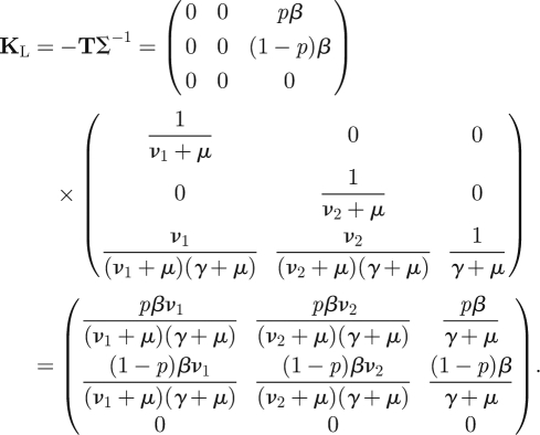As we will show formally in §3, the dominant eigenvalue of this matrix is equal to ℛ₀, where

2.10

Interlude: From a computational point of view, it is easy to use a mathematical software package to compute K_L from T and Σ. We remark, however, that the only cumbersome step, i.e. computing the inverse of Σ, can be easily performed using the biological interpretation of −Σ⁻¹. In, for example, Diekmann & Heesterbeek (2000, p. 35) it is shown that the element (−Σ⁻¹)_ij is the expected time that an individual who presently has state j will spend in state i during its entire future ‘life’ (in the epidemiological sense). In the above example this works out as follows. Individuals who are presently in state E_i will spend, on average, an amount of time 1/(ν_i + μ) in that state. The same individuals will spend on average an amount of time (ν_i/(ν_i + μ)) × (1/(γ + μ)) in state I, where the first factor is the probability that an individual actually changes its state from E_i to I, instead of leaving state E_i by dying, and the second factor is the average amount of time an individual who enters state I spends in state I.³ The individuals in state E_i will spend no time at all in state E_j, with j ≠ i, leading to zeros for the appropriate elements. Finally, individuals who are presently in state I will spend no time at all in states E₁ and E₂, and will, on average, spend an amount of time 1/(γ + μ) in state I. This leads to a full specification of −Σ⁻¹.

We now proceed with our exposition. The first thing to note is that T has a special structure: the third row of T consists of zeros only. Individuals can therefore not be in the third state (in this case state I) immediately after infection. Hence the system has only two states-at-infection: all individuals start their infected life (i.e. are epidemiologically born) in either E₁ or E₂. The NGM is therefore a two-dimensional matrix.

The formal approach to obtaining K from K_L is as follows. We pre- and post-multiply K_L by an auxiliary matrix E that singles out the rows and columns relevant for the reduced set of states. Specify E as consisting of unit column vectors e_i, for all i such that the ith row of T is not identically zero.⁴ In other words, create a matrix E whose columns consist of unit vectors relating to non-zero rows of T only. In the above case this leads to

To find the NGM we then perform the matrix multiplication

2.11

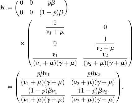
For the example above, we get for the product of E′T and −Σ⁻¹E

Remember that for a 2 × 2 matrix the dominant eigenvalue, and hence ℛ₀, can be obtained from the trace and the determinant of the matrix as

2.12

Note that, in our example, det K = 0, i.e. K is a singular matrix. Because K is a 2 × 2 matrix we can conclude right away that ℛ₀ = trace K. The resulting expression is as in equation (2.10) above.

Apart from resulting in a simplified expression for ℛ₀ in the two-dimensional case, an NGM with the property that det K = 0 has the added feature that we can achieve further reduction in dimension of the matrix. We return to this below. First we show that, by epidemiological reasoning directly from the specification of the system, we can obtain the elements of K from their interpretation without going through the linear algebra. For initial training in this kind of argument it helps to draw a diagram of the system one is studying. For our example above the argument goes as follows. For the element K₁₁, we start with one individual with state-at-infection 1 (i.e. an individual who has just entered state E₁), and determine, by following that individual for the remainder of its infectious life, how many new cases of state-at-infection 1 it is expected to produce. Before the individual can infect, it has to survive the E₁ state and move to the I state. This happens with probability ν₁/(ν₁ + μ). While in the I state, the individual is expected to produce new cases at a rate β, for an expected time 1/(γ + μ). A fraction p of these will be new cases with state-at-infection 1. Multiplying these factors gives

Analogous reasoning gives the expressions for K₁₂, K₂₁ and K₂₂.

In this example we saw that det K = 0. The special feature of the model that causes this is that the states-at-infection are necessarily produced in a fixed proportion.⁵ One can then reduce the dimension of the system even further than the reduction from the three-dimensional K_L to the two-dimensional K. In this example, we need only one state to fully determine ℛ₀, because there is only one state in which individuals can produce new cases, i.e. state I. We will call a state where individuals can produce new cases state-of-infectiousness. This argument can be formalized by defining an NGM with small domain K_S for such situations. To see whether the dimension of K_S is smaller than the dimension of K we can simply check whether det K = 0.

To determine K_S from K, when a reduction is possible, we again examine the transmission matrix T, but instead of only examining the rows we now also examine the columns. For the example above we see that T has two columns containing only zeros, and only one column that is a non-zero vector. All three columns are therefore multiples of the same vector C ≔ (p, 1 − p, 0)′, the first two columns being zero times this vector, the third column being β times this vector. Similarly, the rows of T are all multiples of one row vector R ≔ (0, 0, β), the first row is p times this vector, the second row is (1 − p) times this vector, and the third row is zero times this vector. Actually, R and C constitute a (multiplicative) decomposition of the transmission matrix T, in the sense that T = CR, i.e. T_ij = C_iR_j. We define the NGM with small domain by

2.13

For this example

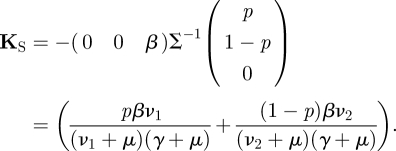The dominant eigenvalue of this ‘matrix’ equals ℛ₀, as given in equation (2.10).

2.2. An SEI model with two host categories

To illustrate the power of our approach, we now briefly consider a similar system but allow the difference between categories 1 and 2 in the population to manifest itself in all states. We then distinguish eight states S₁, S₂, E₁, E₂, I₁, I₂, R₁ and R₂, making the system originally six-dimensional. (The sizes of the subpopulations of those that belong to categories 1 and 2 are constant at pN and (1 − p) N, respectively.) The equations for this system are

Reasoning as in §2.1, we see that there are four infected states in this system, and we restrict ourselves to a four-dimensional infected subsystem. The transmission and transition matrices of the corresponding linearized subsystem are four-dimensional, with

and

The NGM with large domain K_L = −TΣ⁻¹ is four-dimensional:

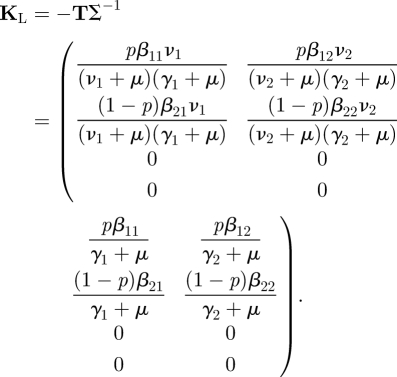Of the four infected states, there are only two that are states-at-infection. We know this from the model, but we can also see this immediately by looking at T and noting that two rows consist entirely of zeros. The NGM K is therefore two-dimensional. The NGM can be found by epidemiological reasoning from the interpretation of its elements in exactly the same way as in §2.1, but replacing the β by the appropriate β_ij in K_ij. If we use the formal linear algebra approach, we again start by examining the transmission matrix T. The two zero rows are rows 3 and 4. Therefore, the auxiliary matrix E will have as its columns the first two unit vectors (1, 0, 0, 0)′ and (0, 1, 0, 0)′:

and

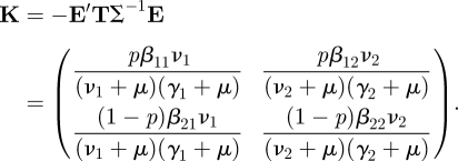We now investigate whether this example allows a further reduction in dimension as in §2.1. We calculate det K and establish that it is, in general, not equal to zero. Therefore no further reduction in dimension is possible, unless β₁₁β₂₂ = β₁₂β₂₁. Due to the fact that we have allowed β_ij to be different for all combinations, we no longer have that the two states-at-infection occur in a fixed ratio.

For ‘completeness’ we note that we can regain such a fixed ratio, and the consequent reduction in dimension, in the special case that β_ij = a_ib_j. Here a_i relates to the susceptibility and b_j to the infectivity (so the idea is that the properties of the two individuals involved in a contact that can lead to transmission have an independent influence). This assumption is called separable mixing in Diekmann & Heesterbeek (2000). It leads to det K = 0, and hence to R₀ = trace K because K is two-dimensional. To proceed formally with this special case via the NGM with small domain, we would write

To find the NGM with small domain, K_S, we observe that the rows of matrix T are multiples of the vector R = (0, 0, b₁, b₂), and the columns are multiples of C = (pa₁, (1 − p)a₂, 0, 0)′. Note that T = CR. We then write

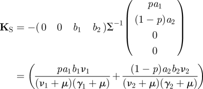and we find

3. Recipes for NGMs

We have now introduced the main concepts of the next-generation approach: the NGM with large domain, the NGM and the NGM with small domain. All three can be derived by simple linear algebra from the basic ingredients T and Σ, or by using the epidemiological interpretation of the NGM. In this section we provide recipes for the construction of these matrices by formalizing the steps we have taken in the examples of the previous section. We show in general that K, K_L and K_S have the same dominant eigenvalue.

3.1. The NGM with large domain

The NGM with large domain, K_L, is always the matrix with highest dimension. Our starting point is the ODE system that describes the production of new cases and the changes in infected states. We assume that this set of ODEs, the infection subsystem, has been written in linearized form. The recipe is as follows.

1. Decompose⁶ the Jacobian matrix of the infection subsystem as T + Σ, where T is the transmission matrix, and Σ the transition matrix:

   • — T contains the entries corresponding to transmission events, where an epidemiological birth occurs, and
   • — Σ contains the entries corresponding to all other changes of state (including death).

2. Compute the NGM with large domain as K_L =−TΣ⁻¹.

The ijth entry of −Σ⁻¹ can be interpreted as the expected time that an individual who presently has infected state j will spend in infected state i (see the interlude in §2.1). Because the ijth entry of T is the rate at which an individual in infected state j produces individuals with infected state i, the ijth entry of K_L = −TΣ⁻¹ is the expected number of infected offspring with state i at infection produced throughout its entire future infected life by an individual presently in infected state j. If there are infected states which are not states-at-infection, the matrix K_L has one or more zero rows. This implies that some of the information contained in K_L is redundant if we are only interested in the growth or decline of the infected population as we iterate K_L. The NGM K is the restriction of K_L to the subset of states-at-infection. Thus this redundancy is removed in K. The interpretation of the entry K_ij of K is the expected number of new infections with state-at-infection i produced by one individual with state-at-infection j.

3.2. The NGM

The NGM, K, has the advantage that it has both a rigorous biological interpretation and excludes irrelevant information. It is usually of lower dimension than K_L. Out of all infected states used for K we select only those that an infected individual can be in immediately after becoming infected. We call these the states-at-infection, and K reflects the restriction of the analysis to the states-at-infection. Essentially, as we showed in the examples in §2 (and will also show for the examples in §4) the interpretation allows one to ‘compute’ K in a rigorous, but biological, manner. Below, however, we present two linear algebra recipes that allow programming. The second recipe uses the computation of the entire matrix −Σ⁻¹ and is the easiest when one uses mathematical software to automate the process. The first recipe uses the epidemiological interpretation and demonstrates that one does not need all elements of −Σ⁻¹ to compute K, some elements will be multiplied by elements of T that are zero and therefore do not contribute. In fact, the second recipe is a programmable version of the first.

The first recipe is as follows.

1. Identify, see §3.1, the transmission matrix T, and the transition matrix Σ.

2. Identify the states-at-infection. State j is a state-at-infection if and only if there is at least one non-zero element in the jth row of matrix T.

3. Identify the states-of-infectiousness. State ℓ is a state-of-infectiousness if and only if there is at least one non-zero element in the ℓth column of T.

4. Compute an auxiliary matrix A which has elements A_ℓj : =− (Σ⁻¹)_ℓj for all ℓj combinations where j is a state-at-infection and ℓ is a state-of-infectiousness, and for which all other elements are zero.

5. Define K_ij = (TA)_ij for all combinations with i and j both states-at-infection.

The second recipe is as follows.

1. Determine if the number of states-at-infection is less than the dimension of the infection subsystem.

   • — If T has no rows consisting entirely of zeros, then K = K_L and proceed with step (ii) in §3.1.
   • — If T has one or more rows consisting entirely of zeros, then K ≠ K_L and proceed as below.
2. Identify the auxiliary matrix E as follows:

   • — The matrix E has the same number of rows as T.
   • — There is one column of E for each non-zero row of T, and hence for each state-at-infection. That column of E has a one in the row that corresponds to the non-zero row of T (state-at-infection), and zeros elsewhere.

3. Compute the NGM, K = −E′ TΣ⁻¹ E.

By definition the basic reproduction number is the largest eigenvalue of the NGM, R₀ = ρ(K). We now show that the NGM and the NGM with large domain have the same non-zero eigenvalues. Let v be an eigenvector of K with corresponding eigenvalue λ. Then Kv = −E′TΣ⁻¹Ev = λv. Multiply this identity by E to get −EE′TΣ⁻¹Ev = λEv. But EE′T = T, so Ev is an eigenvector of K_L with corresponding eigenvalue λ, and the non-zero eigenvalues of K and K_L are the same. (Note that it is impossible that Ev = 0 because this would imply that λv = Kv = 0, hence v = 0 as λ ≠ 0.)

3.3. The NGM with small domain

The NGM with small domain, K_S, has the lowest dimension of the three types of NGM discussed. In many cases, however, it will be equal to K. If det K = 0, the NGM with small domain is different from K. This will certainly be the case if there are fewer states-of-infectiousness than states-at-infection, as in the example in §2.1 above (and in the example in §4.2). Indeed, in that case it makes perfect sense to define a matrix K_S with elements K_Sij = −(TΣ⁻¹)_ij, with both i and j restricted to states-of-infectiousness. It simply means that we focus our bookkeeping on individuals who have just entered a state-of-infectiousness, and compute how many of their epidemiological offspring will enter, on average, the various states-of-infectiousness. In other words, we base our bookkeeping not on being born, but on the later phase in the ‘epidemiological life’ where the individual starts to reproduce.⁷

As the example presented in §2.2 shows, there may be other reasons why det K = 0. We now give a general recipe to derive K_S from K (in a manner that works whatever the reason is that det K = 0). The recipe is as follows.

1. Follow the recipe in §3.2 to determine K.

2. Determine whether det K = 0.⁸

   • — If det K ≠ 0 then no further reduction is possible and K_S = K.
   • — If det K = 0 proceed as below.

3. Define a matrix R, whose rows are linearly independent vectors spanning the rows of T, and a matrix C, whose columns are linearly independent vectors spanning the columns of T. Scale the matrices so that T = CR.

4. Compute the NGM with small domain, K_S = −RΣ⁻¹ C.

As a side remark we now explain that one can derive K_S from K in more or less the same way as we derived K from K_L. When deriving K, we consider ‘pure’ states-at-infection and represent these in the columns of E. A more general point of view considers ‘mixed’ states-at-infection, by which we mean a probability distribution for state-at-infection represented by a column with non-negative elements that sum to one (and with zero elements, of course, at positions that do not correspond to states-at-infection). By replacing E by a matrix consisting of such probability vectors, one may derive K_S directly from −TΣ⁻¹, following the recipe in §3.2.

We now show that the NGM with small domain and the NGM with large domain have the same non-zero eigenvalues. Let v be an eigenvector of K_S with corresponding eigenvalue λ. Then K_S v =−RΣ⁻¹ Cv = λv. Multiply this identity by C to get −CRΣ⁻¹ × Cv = λCv. But CR = T, so Cv is an eigenvector of K_L with corresponding eigenvalue λ. As the matrices K, K_L and K_S have the same rank, we have established that they have the same non-zero spectrum and hence the same dominant eigenvalue.

4. Examples

To illustrate our method further, we present three more examples, each highlighting special difficulties one might encounter. For the first example we analyse a sexually transmitted infection of SEI type, which we then extend by adding vertical transmission of infection. The final example is taken from the literature and based on a model for the transmission of bovine viral diarrhoea. For each example we start with the infection subsystem.

4.1. A sexual transmission SEI model

Consider a purely heterosexually transmitted infectious disease. If the numbers of exposed and infectious females are E₁ and I₁, and the numbers of exposed and infectious males are E₂ and I₂ respectively, then we assume that

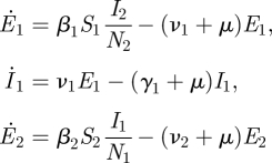where N₁ and N₂ are the sizes of the subpopulations of females and males, respectively. To construct the NGM K, observe that a newly infected male (in the E₂ state or with state-at-infection E₂) has a probability ν₂/(ν₂ + μ) of entering the I₂ state, and would then infect females at a rate β₁N₁/N₂ over a period of 1/(γ₂ + μ) time units. Hence the entry in row one column two. A similar argument specifies the entry in row two column one. We have deduced that

4.1

Hence we obtain the expression for ℛ₀ directly from the formula (2.12) with trace K = 0:

4.2

This example illustrates how easy it is to write down the NGM directly from epidemiological reasoning. As the NGM is two-dimensional it is then straightforward to compute ℛ₀.

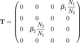
For the more laborious way of using the recipe one proceeds as follows. Specify, from the infection subsystem, the transmission matrix as

and the transition matrix as

Then calculate

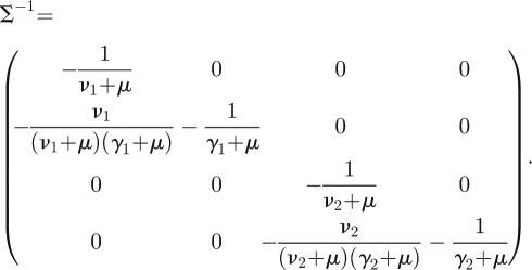The NGM with large domain is given by K_L = −TΣ⁻¹ and is four-dimensional. Using the second recipe in §3.2, we observe that the matrix T has only two non-zero rows, the first and third, so the auxiliary matrix E is given by

and the formula K = −E′TΣ⁻¹E then leads to equation (4.1) above. Note that det K ≠ 0, so no further reduction of dimension (K to K_S) is possible.

4.2. A model for a sexually transmitted infection with vertical transmission

Now consider an SI model for a heterosexually transmitted infectious disease that may also be transmitted vertically. As new-born individuals are not immediately sexually active, we take J₁ and J₂ to be the numbers of infected juvenile females and males, and I₁ and I₂ to be the numbers of infected adult females and males, respectively. We assume that both the length of the pre-sexual period and the length of the infectious period are large compared to the latency period, so we neglect the latter. We also assume that the sex ratio of offspring is one-to-one (a logical consequence is that N₁ = N₂ if the per capita death rates are equal, but we shall keep the quasi-generality of allowing these numbers to be different). We are thus led to consider the following infected subsystem:

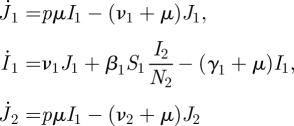where p denotes the probability that a vertical transmission takes place when offspring is produced.

There are four states-at-infection: vertically infected females J₁; horizontally infected females (included in I₁); vertically infected males J₂; and horizontally infected males (included in I₂). A horizontally infected female is initially in the I₁ state. She produces vertically infected females and males at rate pμ and horizontally infects males at rate β₂N₂/N₁, all for a period of, on average, 1/(γ₁ + μ) time units. Hence the second column of K, specified in equation (4.3). A vertically infected female enters the I₁ state with probability ν₁/(ν₁ + μ), hence the first column of K is just a multiple of the second. A horizontally infected male is initially in the I₂ state, and horizontally infects females at the rate β₁N₁/N₂ for a period of 1/(γ₂ + μ) time units, hence the K₂₄ entry. This is the only way that a male transmits the infection, so the other entries in the fourth column of K are zero. Finally, a vertically infected male enters the I₂ state with probability ν₂/(ν₂ + μ), and the third column of K is a multiple of the fourth. Note that all of these expressions concern a fully susceptible population. The NGM for this model is

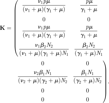4.3

The NGM is four-dimensional, but of rank two and hence has two zero eigenvalues.

We have shown how the NGM is easily constructed by epidemiological reasoning. Alternatively, we may proceed using the linear algebra recipe. We observe that the transmission and transition matrices are, respectively,

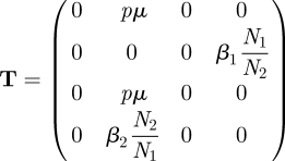and

As T has entries in all four rows, each infected state is, in this example, a state-at-infection. Because there are no zero rows the matrix E consists of all four unit vectors and therefore equals the identity matrix. Hence for this example K = K_L = −TΣ⁻¹.

Note that, from T, it is easily seen that among the four states-at-infection, there are only two that are also states-of-infectiousness: only the second and fourth columns of T contain at least one non-zero element. The columns correspond to state I₁ and I₂, which can, of course, also be gleaned from the biological interpretation of the four states.

So det K = 0, and reduction to an NMG with small domain is possible. The matrix K_S has eigenvalues equal to the two non-zero eigenvalues of K. To formally construct the matrix K_S we observe that the rows of matrix T are spanned by the vectors (0, 1, 0, 0) and (0, 0, 0, 1); and the columns are spanned by (pμ, 0, pμ, β₂N₂/N₁)′ and (0, β₁N₁/N₂, 0, 0)′. We then define matrices

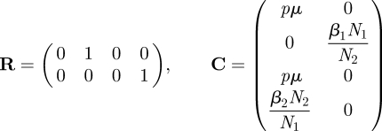and write

The basic reproduction number can be obtained easily from the formula for 2 × 2 matrices (equation (2.12)) applied to K_S:

4.3. A model for bovine viral diarrhoea

A modified SEIR model for bovine viral diarrhoea was described by Cherry et al. (1998). The system has both horizontal and vertical transmissions. Horizontally infected animals can be in E, I and R states. Animals that have been pregnant for less than 150 days when becoming infected may, following recovery into one particular immune state Z of several possible immune states, give birth to an infected calf. These offspring are classified as persistently infected (P state): they transmit infection, give birth at a lower rate and die at a higher rate than cattle that were infected by the horizontal route. Let the constant p₁ be the probability that an infected animal enters the immune state Z upon recovery, let p₂ be the probability that an infected foetus survives to enter the herd, 1/α be the average time spent carrying an infected foetus, and a and b be the reduction in birth rate and increase in death rate of persistently infected animals, respectively.

With a change in notation from Cherry et al. the model is described by

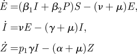where, as before, we restrict ourselves to the infected subsystem. Note, however, that there is a difference with the previous examples that included a recovered state. In the previous examples the R state did not occur in the equations for the infected states and could therefore be ignored for the construction of the NGM and the calculation of ℛ₀. Individuals in an R state do not give rise to new infections, so R is considered to be a non-infected state. In this particular example this is still true as far as horizontal transmission is concerned and for all immune states in the model (not shown here) other than state Z. It is, however, not true that recovered individuals cannot produce new infections in this model, because vertical transmission occurs from immune state Z. Calves are born after the mother has recovered from the infection, and therefore recovered mothers in state Z can give rise to new infections through birth. There are therefore four infected states. The transmission and transition matrices are

and

We omit the computation of the four-dimensional K_L. Note that T has non-zero elements in two rows only, hence K is two-dimensional. The two states-at-infection are the horizontally infected E state and the vertically (and persistently) infected P state. Define

Then the NGM is given by

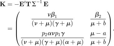The basic reproduction number is then calculated easily from K using equation (2.12).

The NGM K can, of course, also be constructed directly from epidemiological considerations as follows. A proportion ν/(ν + μ) of those horizontally infected become infectious, and infect others at the rate β₁ for, on average, 1/(γ + μ) time units. A proportion p₁γ/(α + μ) of these enter the Z state, and give birth to persistently infected calves at rate p₂α for, on average, 1/(μ + b) time units. Hence the first column of K is obtained. To construct the second column, observe that those in the persistently infected state infect others horizontally at rate β₂, and give birth to persistently infected calves at rate μ − a for 1/(μ + b) time units. So we see, once again, that a simple epidemiological argument may be used to directly construct the NGM K.

5. Conclusion

In epidemic models, individuals can typically be in a number of different states, reflecting both differences in traits and differences in infection status. From the states that apply to infected individuals, we single out those states that individuals can be in immediately after they have been infected. We call these states-at-infection. They play a special role in the definition and calculation of ℛ₀ as the dominant eigenvalue of the NGM associated with the epidemic system. The NGM has an appealing epidemiological interpretation because its components may be regarded as ℛ₀-like quantities. We have provided a recipe for the construction of the NGM for general compartmental epidemic models, exploiting also that there may be only a few states-of-infectiousness in a given system. The recipe may be implemented easily in commonly used mathematical software.

We have in fact given three recipes because we have identified three different NGMs and have clarified the relationships between them. This is useful because some researchers have been confused when trying to reconcile an existing algorithmic linear algebra approach (Diekmann & Heesterbeek 2000, pp. 105–107; Van den Driessche & Watmough 2002) with the original approach using the epidemiological interpretation. We show that the reason is that the approaches lead to two different matrices, which we now call the NGM and the NGM with large domain. Both of these matrices have ℛ₀ as their dominant eigenvalue, the difference lies in the set of individual states that the matrices reflect. We have provided easy algorithms for the construction of the matrices. Both algorithms start by identifying transmission and transition matrices from the linearization of the compartmental model near the infection-free steady state: the transmission matrix describes the production of new infections, and the transition matrix describes changes of infected states (including removal by death or recovery). The NGM with large domain is obtained by a direct construction using these two matrices. By identifying the subset of epidemiological states-at-infection, which is easily done by examining the transmission matrix, we use the second recipe to find the NGM proper. It is often of lower dimension than the NGM with large domain, leading to a simpler calculation of ℛ₀. Sometimes it is possible to construct the NGM with small domain. This matrix may have a less readily understandable interpretation in terms of the epidemiology, but has the advantage of a lower dimension.

Although we present three mathematical recipes, we encourage the construction of the NGM from epidemiological reasoning. This is straightforward and maintains the connection between the mathematics and the biology, and especially gives the user a fuller understanding of the interpretation of the results.

Appendix A. A proof that ℛ₀ governs the stability of the infection-free steady state

Before formulating the key hypotheses concerning T and Σ we introduce some notation. For a square matrix A we denote by s(A) the spectral bound and by ρ(A) the spectral radius:

and

where σ(A) denotes the spectrum of A, that is the set of eigenvalues. All matrices that we consider have real entries. As customary, we call a non-zero matrix A positive if all entries are non-negative; and positive-off-diagonal if all entries are non-negative except possibly those on the diagonal. The following holds if A is a positive-off-diagonal matrix: s(A) < 0 if and only if A is invertible and −A⁻¹ is a positive matrix (for a proof see, for example, lemma 6.12 in Diekmann & Heesterbeek (2000)).

In the following we assume that T is a positive matrix, and that Σ is a positive-off-diagonal matrix with s(Σ) < 0, hence −Σ⁻¹ is a positive matrix. These assumptions reflect the biological meaning of both matrices; the condition s(Σ) < 0 reflects that one cannot remain (potentially) infectious for ever.

For the proof it is convenient to take the NGM with large domain K_L as our starting point; the equivalence of the spectral radius of K_L and K, as shown in §3, then confirms the result for the NGM K. The basic reproduction number ℛ₀ is defined by

The stability of the zero steady state of the linear system

is determined by the sign of the Malthusian parameter r, which is defined as

This criterion extends to the nonlinear system by the principle of linearized stability if, in addition, the demographic dynamics make the infection-free steady state stable in the invariant subspace corresponding to the absence of the infectious agent. The key result of this appendix is the following.

Theorem A.1. —

Let T be a positive matrix and let Σ be a positive off-diagonal matrix with s(Σ) < 0. Let ℛ₀ = ρ(−TΣ⁻¹) and r = s(T + Σ). Then the following equality holds:⁹

We first prove the result under the extra assumptions that T + Σ is irreducible and ℛ₀ > 0, and then employ an approximation and continuity argument to establish the result in general. The proof is based on ideas in Li & Schneider (2002), who addressed a similar problem in population dynamics in a discrete-time setting. In Van den Driessche & Watmough (2002) a proof is presented in terms of M-matrices, and we refer to Thieme (2009) for the analogous result for the infinite dimensional case.

Lemma A.2. —

If ℛ₀ > 0 then s(ℛ₀⁻¹ T + Σ) = 0.

Proof. —

First assume that T + Σ is irreducible. Let v be the non-negative left eigenvector of K_L = −TΣ⁻¹ corresponding to the eigenvalue ℛ₀. Hence vK_L = ℛ₀v which can be rearranged to obtain

A 1

The irreducibility of T + Σ implies that ℛ₀⁻¹ T + Σ is irreducible. By adding a large positive multiple of the identity, kI, to ℛ₀⁻¹ T + Σ, we obtain a positive irreducible matrix, and since v is non-negative it must be the eigenvector corresponding to the spectral radius of that matrix. It follows that all the other eigenvalues have smaller real parts. By subtracting kI again all eigenvalues shift to the left in the complex plane, but the order relation between their real parts remains intact. Hence we conclude from equation (A 1) that s(ℛ₀⁻¹T + Σ) = 0.

Next consider the case that T + Σ is reducible. Regard the irreducible matrix T + ϵ1 + Σ, where 1 is the matrix with all entries equal to one. Denote the spectral radius of the matrix −(T + ϵ1)Σ⁻¹ by ρ_ϵ. For ϵ ↓ 0, we have that ρ_ϵ → ℛ₀ and hence ρ_ϵ> 0 for ϵ small. So, by the above proof for the irreducible case, s((T + ϵ1)/ρ_ϵ + Σ) = 0. Finally, for ϵ ↓ 0 we have, as noted above, that ρϵ → ℛ₀, and hence s(T/ℛ₀ + Σ) = lim_ϵ→0 s((T + ϵ1)/ρ_ϵ + Σ) = 0. ▪

Lemma A.3. —

If T + Σ is irreducible then

is strictly monotone decreasing.

Proof. —

We first add kI to T + Σ for some k large enough to obtain a positive matrix. The spectral radius of an irreducible positive matrix strictly decreases (increases) if any entry of that matrix decreases (increases) (see theorem 2.1 in Li & Schneider (2002) and references therein). Hence the spectral radius of y⁻¹T + Σ + kI is a monotone function of y. For a positive matrix the spectral radius is equal to the spectral bound, and it remains equal to the spectral bound as the spectrum shifts to the left when we subtract kI. ▪

Lemma A.4. —

If T + Σ is irreducible and ℛ₀ > 0 then sign (r) = sign(ℛ₀ − 1).

Proof. —

If ℛ₀ > 1 then (by lemma A.3) s(T + Σ)> s(ℛ₀⁻¹T + Σ), but (by lemma A.2) s(ℛ₀⁻¹T + Σ) = 0, hence r = s(T + Σ) > 0. If ℛ₀ = 1 then (by lemma A.2) r = s(T + Σ) = 0. If ℛ₀ < 1 then (by lemma A.3) s(T + Σ)< s(ℛ₀⁻¹T + Σ), by lemma A.2 s(ℛ₀⁻¹ T + Σ) = 0, hence r = s(T + Σ)< 0.▪

Lemma A.5. —

If s(T + Σ) = 0 then ℛ₀ ≥ 1.

Proof. —

By the shifting argument used above, it follows that s(T + Σ) is an eigenvalue of T + Σ. Let u ≠ 0 be a vector such that (T + Σ)u = 0, and define v = Σu. As Σ is invertible, v ≠ 0. Moreover, (TΣ⁻¹ + I)v = (T + Σ)u = 0, hence K_L = −TΣ⁻¹ has a unit eigenvalue and the spectral radius of K_L must be greater than or equal to one.▪

Lemma A.6. —

If s(T + Σ) = 0 then ℛ₀ = 1.

Proof. —

Below we approximate K_L = −TΣ⁻¹ with a continuous family of matrices, parametrized by ϵ, that have spectral radius less than or equal to one for ϵ > 0, and which converge to K_L as ϵ ↓ 0. It follows that ℛ₀ ≤ 1. Because from lemma A.5 it follows that ℛ₀ ≥ 1, we conclude that ℛ₀ = 1.

Define A(ϵ) = T + Σ + ϵ1, where 1 is the matrix with all entries equal to one. From similar arguments to those used in the proof of lemma A.3, it follows that the function ϵ ↦ s(A(ϵ)) is monotone increasing. So, if we define Ã(ϵ) = A(ϵ) − s(A(2ϵ))I, then s(Ã(ϵ)) = s(A(ϵ)) − s(A(2ϵ)) ≤ 0. The decomposition Ã(ϵ) = (T + ϵ1) + (Σ − s(A(2ϵ))I) motivates us to introduce the matrix

Clearly, M(ϵ) converges to K_L as ϵ ↓ 0, and as the spectral radius of K_L exceeds one (by lemma A.5), the spectral radius of M(ϵ) must be positive for small positive ϵ. Because Ã(ϵ) is clearly irreducible, we use lemma A.4 to deduce that ρ(M(ϵ)) ≤ 1.▪

Proof of theorem A.1. —

Combining lemmas A.6 and A.2 (with ℛ₀ = 1) we conclude that

By lemma A.4 we have that, at least for small ϵ > 0,

and so, by considering the limit ϵ ↓ 0 that s(T + Σ) < 0 ⇒ ℛ₀ ≤ 1 and ℛ₀ < 1 ⇒ s(T + Σ) ≤ 0. Since, as already noted above, s(T + Σ) = 0 ⇔ ℛ₀ = 1, we conclude that s(T + Σ)< 0 ⇔ ℛ₀ < 1. It follows that s(T + Σ)> 0 ⇔ ℛ₀ > 1, and the proof is complete.▪

References

- Cherry B. R., Reeves M. J., Smith G. 1998. Evaluation of bovine viral diarrhea virus control using a mathematical model of infection dynamics. Prev. Vet. Med. 33, 91–108. ( 10.1016/S0167-5877(97)00050-0) [DOI] [PubMed] [Google Scholar]
- Diekmann O., Heesterbeek J. A. P. 2000. Mathematical epidemiology of infectious diseases: model building, analysis and interpretation. Chichester, UK: Wiley. [Google Scholar]
- Diekmann O., Heesterbeek J. A. P., Metz J. A. J. 1990. On the definition and computation of the basic reproduction ratio ℛ0 in models for infectious diseases in heterogeneous populations. J. Math. Biol. 28, 365–382. ( 10.1007/BF00178324) [DOI] [PubMed] [Google Scholar]
- Inaba H., Nishiura H. 2008. The state-reproduction number for a multistate class age structured epidemic system and its application to the asymptomatic transmission model. Math. Biosci. 216, 77–89. ( 10.1016/j.mbs.2008.08.005) [DOI] [PubMed] [Google Scholar]
- Li C.-K., Schneider H. 2002. Applications of Perron–Frobenius theory to population dynamics. J. Math. Biol. 44, 450–462. ( 10.1007/S002850100132) [DOI] [PubMed] [Google Scholar]
- Thieme H. R. 2009. Spectral bound and reproduction number for infinite-dimensional population structure and time heterogeneity. SIAM J. Appl. Math. 70, 188–211. ( 10.1137/080732870) [DOI] [Google Scholar]
- Van den Driessche P., Watmough J. 2002. Reproduction numbers and sub-threshold endemic equilibria for compartmental models of disease transmission. Math. Biosci. 180, 29–48. ( 10.1016/S0025-5564(02)00108-6) [DOI] [PubMed] [Google Scholar]