What role does natural selection play in speciation?

Abstract

If distinct biological species are to coexist in sympatry, they must be reproductively isolated and must exploit different limiting resources. A two-niche Levene model is analysed, in which habitat preference and survival depend on underlying additive traits. The population genetics of preference and viability are equivalent. However, there is a linear trade-off between the chances of settling in either niche, whereas viabilities may be constrained arbitrarily. With a convex trade-off, a sexual population evolves a single generalist genotype, whereas with a concave trade-off, disruptive selection favours maximal variance. A pure habitat preference evolves to global linkage equilibrium if mating occurs in a single pool, but remarkably, evolves to pairwise linkage equilibrium within niches if mating is within those niches—independent of the genetics. With a concave trade-off, the population shifts sharply between a unimodal distribution with high gene flow and a bimodal distribution with strong isolation, as the underlying genetic variance increases. However, these alternative states are only simultaneously stable for a narrow parameter range. A sharp threshold is only seen if survival in the ‘wrong’ niche is low; otherwise, strong isolation is impossible. Gene flow from divergent demes makes speciation much easier in parapatry than in sympatry.

1. Introduction

The role of natural selection in the origin of species has been controversial ever since Darwin published his great work in 1859; as can be seen from the papers in this volume, it remains so. Darwin (at least, in the first edition of The origin of species) relied on selection as the main cause of evolutionary change, but saw that hybrid sterility could not be directly selected; instead, he argued that it arises as a side-effect of divergence. In contrast, Wallace's (1889) enthusiasm for selection led him to argue that not only could it strengthen prezygotic isolation, by what we now call reinforcement, but that group selection could even cause hybrid sterility (Cronin 1991, ch. 16). Then, as now, ecological divergence that allows distinct species to live together in sympatry received less attention than reproductive isolation. However, Darwin (1859, ch. 4) did attach great importance to diversifying selection in driving speciation.

This paper begins by briefly reviewing the various roles that selection plays in speciation, but then focuses on how it leads to sympatry, by selecting for reduced recombination and for the use of different limiting resources. Specifically, it argues that the condensation of a single population into two reproductively isolated clusters, coexisting in different niches, is a process distinct from the traditional view of reinforcement and that this process is much more likely to occur in parapatry than in sympatry.

(a). The role of natural selection in speciation

Selection against hybrids is essential to the definition of biological species. Alleles will be eliminated from a population if they find themselves in unfit heterozygotes or recombinants, and similarly, sexual selection will act against alleles that make males unattractive, or make it harder for females to find a mate. The fundamental opposition of selection to the evolution of reproductive isolation has long been seen as the major obstacle to speciation (Darwin 1859, ch. 8; Huxley 1860; Mayr 1963, ch. 17); in Wright's (1932) metaphor of an ‘adaptive landscape’, reproductive isolation corresponds to a valley of reduced mean fitness that cannot be crossed by selection alone. This view motivated a variety of models in which random drift overcomes selection, to knock populations onto new fitness peaks: various models of founder-effect speciation (Mayr 1963, ch. 17; Carson & Templeton 1984), chromosomal speciation (Wright 1941; White 1978) and Wright's (1932) ‘shifting balance’.

In fact, selection will not oppose the evolution of reproductive isolation if that isolation is not expressed during divergence. Separate populations will diverge, even if they experience identical environments: they will not fix the same alleles from the ancestral population and will not pick up the same set of mutations. So, two populations will come to differ at many sites, some fraction of which will affect fitness. Novel genotypes will be produced from crosses between populations that have been separated by only a few thousand generations. A priori, we expect that genotypes that have never been tested by selection would have lower fitness, on average, and that the average hybrid fitness would decrease with divergence. It is remarkable that, in fact, organisms that offer by thousands of amino acid substitutions often freely hybridize, and that even where they do not, relatively few incompatibilities may be responsible for hybrid unfitness (Orr & Turelli 2001). The slow accumulation of reproductive isolation reflects the robustness of organisms to genetic change.

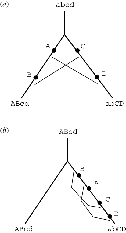
The first explicit models in which reproductive isolation evolves as a side effect of divergence were made by Poulton (1903) and Bateson (1909), and rediscovered by Dobzhansky (1937) and Muller (1942); see Orr (1996). Two alleles arise, one in each lineage, and although each allele is favourable on the ancestral background, they are incompatible with each other. Orr (1995) and Orr & Turelli (2001) generalized these models by supposing that there is some small probability that any pair of alleles will substantially reduce fitness. (Note that there may be incompatibilities between derived alleles in different lineages, or between ancestral and derived alleles in the same lineage; the root could lie anywhere on the path connecting the present-day populations; figure 1.) Orr & Turelli (2001) assume that there is a highly skewed distribution of fitness effects, with a very small fraction of allelic combinations showing large detrimental effects. This is consistent with the results of Drosophila speciation genetics, but remains to be firmly demonstrated more generally, for a wider range of traits and taxa.

Figure 1.

(a) Mutations A and B arise in one lineage, and C and D in another. The descendant populations have genotype ABcd and abCD, and are separated by two Dobzhansky-Muller incompatibilities (DMIs), indicated by thin lines: allele A is incompatible with D, and B with C. Both incompatibilities are between two derived alleles. (b) If the ancestral genotype were ABcd, and four mutations occurred in one lineage (B → b, A → a, c → C, d → D), then the descendant populations would have the same genotypes, but both incompatibilities would be between a derived and an ancestral allele. All that has changed is the position of the root.

It is unfortunate that the term ‘Dobzhansky–Muller incompatibility’ (DMI) is used in a variety of ways: to refer to Dobzhansky and Muller's specific two locus model; to Orr and Turelli's generalization of it; or to the broad idea that reproductive isolation need not be expressed during divergence. It is also not clear whether the term refers to the process of divergence (in which selection does not oppose the evolution of reproductive isolation) or to the outcome (in which a small number of incompatibilities are involved in hybrid breakdown). This paper uses the term ‘broadly’, to refer to an incompatibility that has evolved without ever having been expressed in the ancestral lineages, but avoids making any restrictive assumptions about the distribution of fitness effects.

In these models, although there is no direct selection for or against reproductive isolation, selection may nevertheless drive divergence in a variety of ways. There may be selection for different favourable mutations in a uniform environment, or different environments may fix different alleles. Both the physical and biological environments may differ, the latter including coevolution between host and pathogen, or selfish genetic elements. The isolation that ensues may be related to the process that was selected or may be due to an entirely different pathway (e.g. autoimmunity in plants (Bomblies & Weigel, 2010), nucleoporins in Drosophila, melanomas in fish (Orr & Presgraves 2000)). Divergence might be due to random drift across a neutral adaptive landscape (Gavrilets & Gravner 1997; Gavrilets 2004), or in opposition to weak selection (e.g. compensatory evolution; Innan & Stephan 2001). However, we might expect strongly selected changes to be more likely to cause reproductive isolation as a by-product. It is striking that in all the examples of ‘speciation genes’ discovered to date, there is evidence for positive selection where this has been tested (mainly, by finding excess rates of amino acid substitution). Under the Dobzhansky–Muller model, whether selection drives biological speciation really depends primarily on the extent to which evolution in general is due to selection.

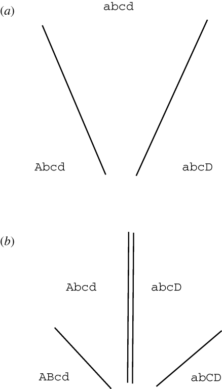
To some extent, it does not matter what causes divergence—the key issue is what fraction of allelic combinations cause incompatibility. However, the cause of divergence is relevant to the geography of speciation. If divergence is due to moderately strong selection, then it can occur despite gene flow. Thus, divergence in parapatry seems just as likely as in allopatry. With discrete demes, selection dominates if it is faster than migration (i.e. s ≫ m), and in a spatially extended population, selection must favour an allele over a spatial scale that is sufficiently large (; Slatkin 1973). As can be seen from the many examples of local adaptation across narrow clines, gene flow does not prevent divergence in a heterogeneous environment. Parapatric divergence is more difficult in a uniform environment, but will still occur if the species covers a broad enough range. Then, favourable alleles will arise at different loci and spread through the range at the same time. If they proved to be incompatible with each other, then they will remain separated by a narrow cline that can be the nucleus for further divergence (figure 2; Kondrashov 2002; Navarro & Barton 2003). The rate of parapatric divergence depends on how long it takes for a favourable allele to sweep through the whole population: the longer it takes, the greater the opportunity for incompatible alleles to meet each other.

Figure 2.

DMIs can accumulate in parapatry as well as in allopatry. (a) Alleles A and D arise at different places, and at different loci, and both begin to spread. (b) If they meet, and are incompatible, then they will remain separated by a stable pair of clines (double lines). New alleles may then arise (B,C); if these are incompatible with each other, or with one of the alleles that are already established, then they will strengthen the isolation, leading to a set of four clines.

Selection plays a much more direct role in the evolution of sympatry—i.e. in determining how divergent populations come to coexist. Yet, this question has been somewhat neglected, relative to the evolution of reproductive isolation. This may be partly because biological species are defined by reproductive isolation, so that on this definition, speciation is identical with the evolution of isolation. It may also be because sympatry requires ecological divergence, so that understanding its evolution depends on combining genetics with ecology and on work in the field rather than the laboratory. Yet, sympatry is essential for the long-term survival of species: otherwise, a species' range will be fragmented into ever smaller areas, until extinction is inevitable. Examples of parapatric distributions, such as chromosomal races in rodents, represent a balance between the accumulation of partial reproductive isolation in parapatry, and the extinction of local races (Patton & Sherwood 1983; Searle 1993).

Alternative combinations of alleles can coexist in sympatry if they use different limiting resources and if they are, to some degree, reproductively isolated, so that recombination is reduced. Neither ecological divergence nor reproductive isolation need be complete, but the net strength of these two factors must exceed some threshold if disruptive selection, favouring the alternative genotypes, is to overcome recombination. (Indeed, in simple models, the sum of these factors is precisely what determines whether coexistence is possible (Udovic 1980; Gavrilets 2004, and see below).)

Recombination can be reduced by assortative mating, by preference for different niches and mating within niches, by selection against intermediate genotypes, or by chromosomal rearrangements. Divergence to use different resources requires some combination of preference and of specialization to better exploit particular resources. So, we need to understand the joint evolution of ecological divergence, postzygotic isolation and prezygotic isolation to give clusters that can ultimately continue their divergence to give full biological species with no gene flow.

This paper refers to ‘habitats’ in a broad sense, to mean the exploitation of a distinct limiting resource; it need not imply a physical location or microhabitat, but could include, e.g. mimicry of different unpalatable model species.

This paper analyses the transition to sympatry by using a generalization of the Levene (1953) model, which assumes soft selection in two habitats; i.e. each habitat produces a fixed proportion of the population, regardless of number that choose to live on each, or the proportion that survive there. Assuming soft selection is a drastic simplification. Ideally, one would allow for separate density-dependent regulation in each habitat, with survival being a decreasing function of numbers. This would allow study of extinction and range limits, but makes the analysis substantially more complicated.

The Levene (1953) model is the basis for a variety of models of sympatric speciation (Maynard Smith 1966; Maynard Smith & Hoekstra 1980; Felsenstein 1981; Diehl & Bush 1989; see Gavrilets 2004, for a review). In particular, Geritz et al. (1998) and Geritz & Kisdi (2000) give an ‘adaptive dynamics’ analysis which is close to that set out here: they assume that viabilities in each niche are a Gaussian function of an underlying trait, and assume a single locus in a diploid sexual population. Recently, Nagylaki (2009) and Bürger (in press) has made a detailed analysis of the multilocus Levene model, but assuming no epistasis.

This paper will lay out the model in a slightly more general way, that allows for multiple loci to interact in order to determine habitat preference and viability in each habitat. This paper will first describe the evolutionarily stable strategy for preference and for viability separately, then show how genes for either may couple together in a single population and finally, extend the analysis to the parapatric case, to ask how initially disjunct populations come to coexist.

2. The Levene model

At the start of each generation, individuals have a probability α_γ of moving into habitat γ. They then have the relative viability v_γ and finally, a fixed fraction c_γ emerge, as breeding adults. Mating may occur randomly within each niche or across the whole population. This paper will focus mainly on the first case, which is more favourable to speciation.

The effects of habitat preference and viability selection on the genotype frequencies within niche γ, g_γ, depend on the product of preference and viability, α_γ(X)v_γ(X):

2.1

and X denotes the genotype. If mixing occurs before mating, we have genotype frequencies g*(X) = ∑_γc_γg_γ(X) in the pool of breeding adults, and the genotype frequency among newborns is ∑_Y,Z R(X, Y, Z)g*(Y)g*(Z); R(X, Y, Z) is the frequency of genotype X among offspring from parental genotype Y,Z. If mating occurs within habitats, we have genotype frequencies among newborns of ∑_γc_γ∑_Y,Z R(X, Y, Z)g_γ(Y)g_γ(Z). After considering the evolutionarily stable strategies (ESS), I will derive explicit results, with R being defined by Mendelian inheritance at multiple loci.

It is crucial to realize that because genotype frequencies change only through the product α_γv_γ, the population genetics of preference and viability are equivalent. Differences arise only to the extent that we assume different constraints: because every individual must go somewhere, it is natural to constrain preferences to sum to 1 (∑_γ α_γ = 1 ∀ X), whereas viabilities in the different habitats could be constrained in a variety of ways. However, if the constraints are the same, then the habitat preference and viability selection change genotype frequencies in the same way.

There is a natural generalization, in which viability is the product of a set of independent components, rather than one; each is determined by a different trait, z_i. If these involve different processes, we can assume that different sets of loci are involved for each. For example, net survival on each habitat might depend on ability to use different nutrients, resistance to different pathogens, development time and so on. Even if alleles of large effect were available for each component, recombination would prevent their coupling together. We do not pursue this idea here, but note that coupling between preference and a single viability trait is similar to coupling among multiple viability traits.

(a). Representing constraints on preference and viability

The habitat preference, α_i, must sum to 1—every individual must go somewhere—and so with two niches, it is convenient to write

2.2

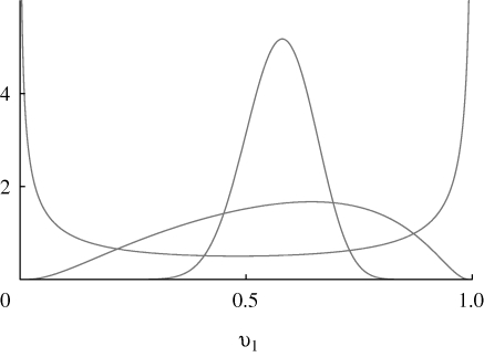
where a is an additive trait (−∞ < a < ∞) that determines the preference. With this choice, the distribution of preference in the population changes from unimodal to bimodal (clustered around 0 and 1) as the variance of a increases (figure 3).

Figure 3.

The distribution of viability, v₁, caused by a normal distribution of the underlying trait, z. This changes from unimodal through to bimodal as the variance in z increases from 0.1 to 1 to 10; mean z = 1, β = 2.

We can write the viability in each niche in a similar way, but now, we must choose the constraint on viabilities in each niche:

2.3

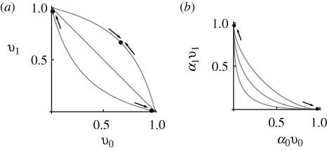
If β > 1, then the trade-off curve (i.e. v₁ considered as a function of v₀) is concave: at z = 0, viability is 1/(1 + β) in both niches, and so is lower than the average viability of an extreme specialist (½ for |z| ≫ 0). Conversely, if β < 1, the trade-off curve is convex, lying above v₀ + v₁ = 1 (figure 4). We will need, below, a more general form, in which the less-well-adapted types always have a minimal viability of at least θ:

2.4

Figure 4.

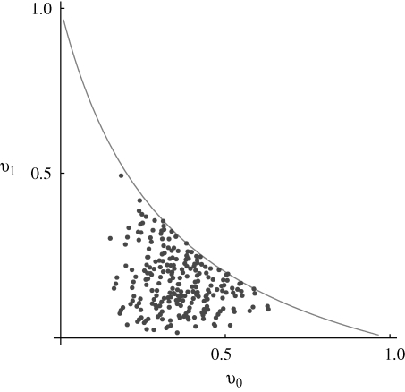
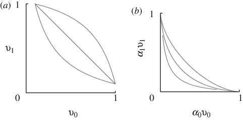
(a) The possible viabilities in each niche are limited by a trade-off curve (equation (2.3)). For β = 1, there is a linear trade-off (v₀ + v₁ ≤ 1; middle line), and any distribution on this line that has mean v̄ = 1 is an ESS. For β = 0.5, the trade-off curve is convex (upper curve), and there is a unique monomorphic ESS for viability (shown at upper right, for c₀ = c₁ = 0.5). Conversely, for β = 2, the trade-off curve is concave, and there is a unique polymorphic ESS, with a mixture of specialist genotypes (dots at upper left, lower right). (b) If both preference and viability vary, and if there is no recombination between them, then what matters is the constraint on the product α_γv_γ. The curves here show the combined trade-off (equation (2.5)) for the viabilities shown in (a), and habitat preference (α₀ + α₁ = 1; equation (2.4)). These are concave, for all β, and so the ESS is always for a polymorphism between two extreme specialists (dots).

It is important to note that this curve represents the outer limit of the set of possible viabilities: genotypes below the curve no doubt exist, but will be less fit than those on the curve. In reality, we can imagine that viability in each niche is controlled by a set of loci with additive effects, with additive trait z_i determining the viability v_i through a logistic relation. Transforming to z_i = log(v_i/(1 − v_i)), the constraint described by equation (2.2) amounts to assuming that z₀ + z₁ ≤ −2 log(β). Thus, we can imagine a set of genotypes whose outer limits lie on the trade-off curve (figure 5). We make the approximation that selection will always take the population onto this curve and neglect deleterious mutations that would take it into the interior. It is thus convenient to assume that alleles lie on the trade-off curve, implying that they have pleiotropic effects. However, this is not a critical assumption: essentially the same results would emerge even if alleles had small effects on viability in only one or other niche (i.e. if there is no pleiotropy). Indeed, it is implausible that alleles would have effects that lie precisely on the trade-off curve.

Figure 5.

The trade-off curve is the outer limit of the set of possible viabilities, {v₀, v₁}: it does not require that mutations have effects that fall on this curve. To illustrate this point, the distribution of genotypic values is shown, for viabilities determined by underlying additive traits {z₀, z₁} (equation (2.2)). These traits are determined as the sum of random effects at 10 loci, with effects on z₀, z₁ at each locus chosen independently from a random uniform distribution, but with the constraint that z₀ + z₁ ≤ 2 log (β); here, β = 2. Selection will take the population close to the trade-off curve.

3. Evolutionarily stable strategies

(a). ESS for habitat preference and viability separately

We begin by finding the ESS for habitat preference and viability separately, by looking for a phenotype that cannot be invaded by any other; this analysis follows Levins' (1968) approach. The ESS preference is when the mean fraction that moves into each niche matches the output of that niche (i.e. ). However, this ESS can be achieved in a variety of ways: there is no selection either for or against variation in preference, because at the ESS, all individuals have the same fitness wherever they go. (For the moment, we are ignoring variation in relative viability between individuals.) Therefore, there may be considerable variation in preference.

Next, consider the ESS for relative viabilities in each niche. If β < 1, giving a convex trade-off curve, then the ESS is for a single generalist phenotype, moderately well adapted to both habitats. Conversely, if β > 1, the ESS is a polymorphism with two specialist genotypes (figure 4). In each case, the ESS maximizes the mean viability, weighted by c_γ; note that because the model assumes a fixed output from each niche, c_γ, the ESS for viability is independent of preference and vice versa: both ESS depend only on the outputs, c_γ.

(b). No recombination: joint ESS for preference and viability

The argument given above is independent of the mode of reproduction, provided that the population is monomorphic. If the population is polymorphic, then the average fitness of an invading allele depends on its association with the existing polymorphism and hence on the rate of recombination. If recombination is so fast, relative to selection, that viability and preference are uncorrelated, then the above arguments for the separate ESS apply. Below, we examine the case where selection and recombination are comparable, so that we must follow the evolution of linkage disequilibrium. First, however, we find the ESS for an asexual population, by finding combinations {α, v} that cannot be displaced.

It is obvious that when any combination of viability and preference can be selected, the ESS will be the coexistence of two perfect specialists: a generalist ESS is only possible when recombination prevents associations between preference and viability from becoming sufficiently strong. However, it is instructive to show this formally, by combining the constraints on preference and trait, to give the joint trade-off curve for their product, α*v, and then asking whether this is concave or convex. Consider α₀v₀ and α₁v₁ as functions of a, z, as given by equations (2.2) and (2.4). Then, by maximizing α₁v₁ for given α₀v₀, we find that the joint trade-off is given by

3.1

Crucially, this is always concave (i.e. α₀v₀ + α₁v₁ < 1 for β > 0 and θ < 1; figures 4 and 6). Thus, even if the trade-off curve for viabilities is convex, so that the ESS for viability is for a single generalist genotype, the joint ESS for preference and trait together is always concave, so that specialists that choose different niches, and are adapted to those niches, will evolve.

Figure 6.

When constraints on preference (α₀ + α₁ = 1) and viability (v₀, v₁) are combined, the trade-off curve for net fitness (α₀v₀, α₁v₁) is always concave. Therefore, in an asexual population, the ESS is always for polymorphism between two extreme specialists, if preference and viability can evolve together. (a) The constraint on viability (equation (2.4)) is convex, straight or concave, depending on whether β = 0.5, 1 or 2 (top right to lower left). (b) The corresponding constraint on net fitness (α_γv_γ) is always concave (θ = 0.1 throughout).

(c). Sexual reproduction

With sexual reproduction, an ESS with polymorphism between extreme specialists is only possible if the genetic system can produce these two extreme types. The simplest case is of a single locus (in diploids, with complete dominance). More elaborate mechanisms include tightly linked ‘supergenes’, or a single locus that switches the effects of other loci between two states. The problem is to understand how such a complex system could evolve: if it cannot, then disruptive selection will maintain a polymorphism that is limited by genetic constraints. Such polymorphism may be maintained at multiple loci, giving an approximately normal distribution of the trait, z; the distribution of viability, v(z), would be roughly normal if the trait variance is small and the trait mean intermediate (figure 3).

We can understand the evolution of a sexual population by assuming that a very large number of loci influence the traits, so that although the extreme phenotypes could be generated, the actual variance is drastically reduced by recombination: reproductive isolation is then strongly favoured, as indeed are any mechanisms that reduce recombination. Assuming that z is tightly clustered around its mean, so that higher-order selection such as ∂² log(v)/∂z² can be neglected, the selection gradient on z can be approximated by E[∂log(v)/∂z], evaluated at the trait mean ; here, the expectation is across niches.

The population will reach an equilibrium for mean z when this gradient is zero; then, the curvature of the fitness landscape determines the outcome. If E[∂²log(v)/∂z²] < 0, then the equilibrium is stable and sexual populations will evolve to that point. At the equilibrium, however, there may nevertheless be disruptive selection, if E[(∂²v/∂z²)/v] > 0. Indeed, for the constraints given in equation (2.3), a sexual population always converges to intermediate z. This is because an extreme specialist has negligible viability in the other niche, so that a variant that has even a very low survival on that niche will gain a huge fitness advantage, being guaranteed the entire output from that niche; nevertheless, if β > 1, the population will be under disruptive selection. Thus, we expect that a sexual population will fix a generalist genotype if β < 1 (or maintain limited genetic variation due to mutation), whereas if β > 1, it will maintain the maximum genetic variance possible, given recombination. This will include a component equal to the maximum at linkage equilibrium, plus an additional component due to linkage disequilibrium, which could be much larger, but which is limited by recombination.

Under equation (2.3), maximum viability in one niche requires zero viability in the other. Then, only a single outcome is possible. In contrast, if the less-well-adapted types have a minimum viability of at least θ > 0 (equation (2.4)), then a sexual population can be selected to specialize on one or the other niche: a variant that does better in the under-used niche must now compete with the predominant type, which has appreciable viability there. Now, there are more possibilities: as well as the evolution of a single generalist phenotype, the ESS may be for specialization on just one niche, or there may be two alternative stable states, with specialization on either one or the other niche.

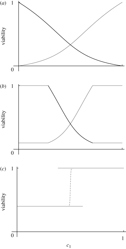
We can understand the various possibilities by thinking of a cline in niche size (c₀, c₁). We ignore dispersal, and so position can be measured by the probability of moving to niche 1, c₁. With θ = 0 (equation (2.3)), a sexual population with low genetic variance will always evolve to an intermediate phenotype that tracks the niche size (figure 7a). If θ > 0, then when niche availability is highly skewed, only specialization on the most abundant niche is stable. When both niches are abundant (c₀ ∼ c₁), there are two possibilities. If β²θ < 1, then for β²θ < c₁/c₀ < 1/β²θ, a single generalist phenotype will evolve, as when θ = 0 (figure 7b). For both these possibilities, intermediate populations will be under disruptive selection if β > 1. If β > β²θ > 1, however, then there is an intermediate region in which there are two alternative stable states: specialization on one or the other niche is stable, but the intermediate generalist equilibrium is unstable. If there is a small amount of migration, then a narrow tension zone will form at the boundary between the alternative states; with uniform density and dispersal, this will move to an equilibrium position at z = 0 (figure 7c).

Figure 7.

(a) The equilibrium viabilities in the two niches, plotted against the size of niche 1, c₁; β = 2, θ = 0. There is a single intermediate equilibrium, which smoothly tracks niche size. (b) With θ = 0.1, populations specialize on the commonest niche when that niche predominates (c₁/c₀ < β²θ, c₁/c₀ > 1/β²θ or c₁ < 0.29, c₁ > 0.71); however, for intermediate c₁, there is an intermediate equilibrium, as in (a). (c) With θ = 0.4, there is an intermediate region with two stable equilibria (0.38 < c₁ < 0.62). If these meet in a cline, a narrow tension zone will form, centred on z = 0 (dashed line). (Only the mean viability in niche 1 is shown here, for clarity.)

Geritz et al. (1998) and Geritz & Kisdi (2000) also find alternative stable states in a model in which viability is a Gaussian function of an underlying trait, rather than a logistic, as used here. The relationship between these models is summarized in appendix A. Note that although we have described the evolution of an additive trait in a sexual population, assuming low genetic variance, the outcome is the same as in an ‘adaptive dynamics’ model, which examines the invasion of new alleles of small effect: in both cases, the outcome depends on the selection gradient near to the current mean.

(d). Selection on modifiers and on linkage disequilibrium

So, we expect there to be variation in habitat preference, because that is not directly selected. For viability, we expect that if there is a concave trade-off between survival on two habitats, and the concavity is strong enough that an intermediate equilibrium exists (i.e. if β² > 1/θ), then disruptive selection will maintain maximum variance in the trait. Selection may then strengthen divergence between habitats in two ways, first distinguished by Felsenstein (1981). First, an allele may be favoured because it reduces the formation of unfit hybrids, by strengthening assortment or by directly reducing recombination, as an adaptive process by which prezygotic isolation evolves in response to postzygotic isolation (Dobzhansky 1940; Servedio & Noor 2003). In the model just outlined, an increased habitat preference would reduce recombination between genotypes emerging from each habitat and so would be favoured. (That is, a modifier that increases the effect of a preference allele and so increases the variance of a would be selected.) Similarly, a modifier that increased the effects of viability alleles, and hence the variance of z, would be favoured. A modifier that reduced recombination would be selected for the same reason (Kirkpatrick & Barton 2006).

In contrast, selection may act to strengthen linkage disequilibrium, rather than to change allele frequencies: different incompatibilities may become coupled together, ultimately leading to distinct clusters. Thus, linkage disequilibrium is expected to develop between habitat preference and viability loci, and between loci within each set. This process, in which different incompatibilities became associated, is fundamentally different from the usual view of reinforcement: it can happen between incompatibilities that act at any stage, including postzygotic as well as prezygotic isolation (Barton & de Cara 2009). Note that selection for both single alleles and for linkage disequilibrium (Felsenstein's (1981) one- and two-allele models) all become more effective as the variance of divergent traits increases. So, we expect a strong feedback, potentially leading to rapid speciation.

We will now analyse the growth of linkage disequilibrium in a single population: first, among preference loci (β = 1) and then among viability loci (β > 1). Finally, we discuss what happens in parapatry, across a cline in niche size.

4. Evolution of linkage disequilibrium

(a). Habitat preference

If there is purely variation in habitat preference (or equivalently, if there is a linear trade-off between viabilities in the two niches), the outcome is remarkably simple. A general analysis is given in appendix A; here, we summarize these results and approximate them using the infinitesimal model.

As explained above, the population evolves to an ESS at which habitat choice matches the output from each niche, so that all genotypes have the same fitness. If mating occurs randomly across the whole population, then the population evolves neutrally, apart from the single constraint that mean preference must match niche size. Thus, the population as a whole evolves to linkage equilibrium, and allele frequencies may drift, as long as the mean preference stays fixed. In general, however, there will be linkage disequilibrium within each niche: unless alleles have multiplicative effects on preference, the set of genotypes that choose to move to one or the other niche will not, in general, be at linkage equilibrium. However, because a separation into different niches, followed by mixing, does not alter genotype frequencies, the population as a whole stays at linkage equilibrium.

If mating occurs within niches, breaking down linkage disequilibria within them, there will nevertheless be strong linkage disequilibrium in the population as a whole, generated by the mixing of divergent populations; this reflects the incipient reproductive isolation caused by mating within separate gene pools. Remarkably, however, pairwise linkage disequilibria tend to zero within niches, regardless of how genotype determines preference and regardless of the pattern of recombination. Thus, the pairwise linkage disequilibrium in the whole population is entirely due to mixing of subpopulations with different allele frequencies. There may, in general, be higher-order linkage disequilibria within niches, which will depend on the genetic map. However, if preference is determined by an additive trait based on at least a modest number of loci, that trait will be normally distributed, with a mean and variance that are independent of linkage disequilibrium; higher-order associations within niches only affect the higher moments of the trait distribution, which are negligible for large numbers of loci.

These results are complementary to those obtained by Nagylaki (2009), who showed that if there is soft selection, mating within demes, and no epistasis, then the population will converge to linkage equilibrium within demes. This result does not require any assumptions about the relationship between selection in different demes (as assumed here, via the trade-off for preference or viability), but does require strict additivity across loci within each deme.

How is it that recombination within habitats, followed by mixing, generates positive linkage disequilibrium in the population as a whole? The preferential movement of different genotypes into different niches does not change genotype frequencies and so does not generate any linkage disequilibrium in the whole population. However, it does generate negative associations within each niche, which are exactly balanced by the positive associations caused by divergence between niches. Thus, if recombination within niches breaks up negative associations, there remains a positive association due to the divergence between subpopulations. (To understand this, think of a simple two-locus example, where the four genotypes are initially equally frequent. With strong preference, all the 00 genotypes and half of the 01 and 10 genotypes will move to one niche, giving genotype frequencies 2∶1∶1∶0. If all linkage disequilibria are eliminated from this subpopulation, then genotype ratios change to 9∶3∶3∶1. After mixing with the other subpopulation (with ratios 1∶3∶3∶9), the overall genotype ratios have changed to 5∶3∶3∶5, showing strong positive linkage disequilibrium.)

When the preference has the particular form of equation (2.3), with β = 1, the ratio between the fitnesses in niche 1 versus niche 0 is e^z, so that the effects of the different loci multiply. In this special case, the equilibrium is in exact linkage equilibrium within niches and is simply described by the allele frequencies within each niche; thus, the ratio of allele frequencies at each locus is just equal to the allelic effect, a, at that locus: (p₁/q₁)/(p₀/q₀) = e^a. The average allele frequency is necessarily p = c₀p₀ + c₁p₁, and so one can solve to find the difference in allele frequency between niches:

4.1

where ã = e^a − 1 measures the allelic effect at that locus. For small effects (a < 1, say), p₁ − p₀ ∼ apq for all c₁; a very large allelic effect (a > 4, say) is required for the allele frequency divergence to approach its maximum value.

If many loci are polymorphic, the trait will follow a Gaussian distribution within each niche and this distribution will not change through random mating and meiosis. The equilibrium then takes a very simple form: the means within each niche are

4.2

where the variance within each niche, V = var(a), is arbitrary and is determined by the underlying allele frequencies. Note that because we assume large numbers of loci here, allele frequencies will only differ slightly between niches, and so we can assume that the variance within each niche is approximately the same. Also, note that although the distribution of the trait within each niche is Gaussian, the distribution of the preference itself is far from Gaussian, since it is bounded between 0 and 1.

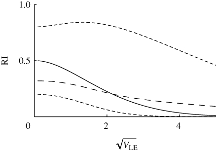
The strength of reproductive isolation can be measured by the probability that a parent that survived to breed in one niche had been born in a different niche. Figure 8 shows how this decreases as the variance in underlying preference increases. The central line is for the symmetric case (c₁ = 0.5). In the asymmetric case (c₁ = 0.2), the chance that a survivor in the commoner niche came from elsewhere is low and decreases rapidly with the variance in preference (lower dashed curve). The chance that a survivor in the rarer niche came from elsewhere is high and surprisingly, gets higher as the variance in preference increases—presumably, because this increases immigration from the commoner niche even more. It does decline for higher variance, but preference has to be exceedingly variable to reduce immigration substantially. Nevertheless, the average chance that a survivor came from elsewhere does decrease with the variance in preference, as expected (central dashed line).

Figure 8.

The probability that a surviving parent in one niche was born in a different niche, plotted against the within-niche variance in underlying preference, var(a). Solid line: symmetric case, c₀ = c₁ = 0.5; dashed lines: asymmetric case, c₀ = 0.2, c₁ = 0.8. The upper dashed line shows the chance that a parent in the smaller niche came from elsewhere, and the lower dashed line, the chance that a parent in the larger niche came from elsewhere. The long dashed line at the centre shows the weighted average of these two. This assumes the infinitesimal model, which has a Gaussian solution (equation (4.2)).

(b). Viability

We now consider a more general trade-off, represented by equation (2.3) with β ≠ 1. If the trade-off curve is convex (β < 1), then selection is stabilizing and a single genotype will fix. We focus on the opposite case (β > 1), where disruptive selection favours maximum variance, subject to the constraint on the mean that is imposed by frequency-dependent selection. Allele frequencies are now no longer neutrally stable and will be kept polymorphic—in the symmetric case, at equal allele frequencies. Selection will also favour positive linkage disequilibria within niches.

We consider the simplest case of unlinked loci with equal allelic effects. Then the frequencies of all genotypes that give the same phenotype can be assumed equal, and we only need to follow the phenotypic distribution. Such symmetric solutions tend to be unstable under disruptive selection, but should be stable to asymmetric fluctuations if selection is disruptive, as we assume here (Barton & Shpak 2000). This simplification makes numerical calculations with up to approximately 50 loci possible.

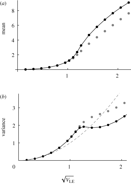
Figure 9 shows an example with n = 40 loci, and β = 2, with equal niche sizes; the mean and variance of z within niche 1 are plotted against the maximum possible standard deviation at linkage equilibrium, = , which increases with the allelic effect, Z. The grey dots show an approximation, based on the assumption that the distribution within each niche is Gaussian. The approximation is calculated by finding how the mean and variance within niches change across one generation and then finding the equilibrium numerically. 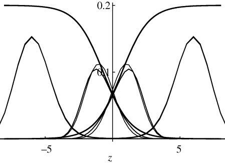This procedure is extremely accurate up until a sharp threshold at , beyond which the Gaussian approximation overestimates the variance and underestimates the mean. Figure 10 shows how the distribution of z in the two niches changes across this transition point. For = 0.95, the distributions overlap and there is substantial gene flow between the niches; the distributions change slightly as a result of reproduction, indicating that there is some linkage disequilibrium, albeit weak. For = 1.6 (outer pair), the distributions do not overlap and each is in linkage equilibrium: reproductive isolation is essentially complete, because the probability of survival in the opposite niche is negligible. It is not obvious why the Gaussian approximation fails as the sub-populations separate: the distribution within niches is still close to Gaussian. The approximation fails because once the distributions have moved so far apart that almost all individuals have high viability in their respective niche, there is then only weak selection on the actual value of z. (To see this, note that the viability (upper curves) is almost constant across the range of each population.) Thus, slight deviations from a Gaussian have large effects on the location of the equilibrium.

Figure 9.

The mean and variance within niches, plotted against the standard deviation at linkage equilibrium, . The dots connected by a solid line show the exact solution, obtained by iterating until convergence. (Starting from linkage equilibrium, and from complete disequilibrium, led to the same values.) Grey dots show the Gaussian approximation. The dashed line in (b) shows the variance at linkage equilibrium, in the population as a whole. There are n = 40 loci, and equal niche sizes; β = 2; values are measured in the newborn population.

Figure 10.

The distributions of the trait, z, within each of the two niches, for standard deviation = 0.95 (inner pair) and 1.6 (outer pair); these correspond to allelic effects Z = 0.3, 0.5, respectively. The upper pair of logistic curves show how the viabilities depend on z. For (outer pair), the distributions before and after reproduction are indistinguishable, implying linkage equilibrium. However, for smaller allelic effects (inner pair), there is appreciable linkage disequilibrium; the solid lines show the distribution within niches immediately before reproduction, and the thin lines, the distribution amongst newborns. Parameters as in figure 9.

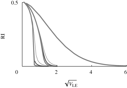
As before, we can measure the strength of reproductive isolation by the chance that a survivor in one niche was born the opposite niche. This is shown in figure 11, which is based on numerical iterations of the symmetrical model, as in figure 9. The rightmost curve is for β = 1, which could represent a pure habitat preference. In this case, calculations for 10, 20 and 40 loci are indistinguishable from each other and from the Gaussian solution to the infinitesimal model (equation (4.2); figure 8); reproductive isolation declines smoothly as the variance in preference increases. The sets of curves to the left are for β = 2 and 4. Now, the number of loci does alter the outcome slightly (compare light with heavy curves in each set), but results do converge with increasing numbers of loci—presumably, to the limiting case of the infinitesimal model.

Figure 11.

The chance that a survivor in one niche was born in a different niche, plotted against the standard deviation at linkage equilibrium , assuming equal allele frequencies. Each set of curves is for β = 1, 2, 4 (right to left); within each set, the three curves are for n = 10, 20, 40 loci (thin to thick lines). Otherwise, parameters as in figure 9.

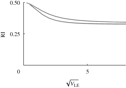
What is most striking is that with strong disruptive selection (β > 1), there is a sharp threshold, beyond which isolation is essentially complete. This can be understood from figure 10: for β ≫ 1, intermediate phenotypes survive poorly in either niche. Therefore, once the distributions within each niche move far enough apart, gene flow almost ceases. This is a consequence of the assumption of a strong trade-off, such that a specialist in one niche has very low fitness in the other. If this assumption is relaxed, by assuming that individuals have a minimal survival of θ = 0.2, however badly adapted they are (equation (2.4)), then strong isolation becomes impossible, and there is no longer a sharp threshold (figure 12). Now, even when the population has very high variance in z (right of graph), a substantial fraction (approx. 0.33 for β = 2) were still born in the other niche. When disruptive selection rises above a threshold , the polymorphic equilibrium becomes unstable, and one or other extreme specialist fixes in the population.

Figure 12.

Reproductive isolation, given that there is a minimum survival θ = 0.2 in the unsuitable niche (equation (2.4)). As in figure 11, this shows the chance that a survivor in one niche was born in a different niche, plotted against . Results for n = 10, 20, 40 loci are indistinguishable. The two curves are for β = 1 (top) and β = 2 (bottom); for = 2.2, the population fixes for one or other specialist.

We began the analysis by showing that an asexual population will evolve to an ESS with coexistence of two specialists, whereas a sexual population with limited phenotypic variance will evolve to an intermediate generalist phenotype that is under disruptive selection if 1< . We might expect that if the genetic variance is free to evolve, and if mating occurs within niches, then both these outcomes could be possible, depending on the starting conditions. A unimodal distribution with low variance could be stable, because the variance would be kept low by recombination, but a bimodal distribution might also be stable under the same conditions, because there would be little gene flow between the two extremes. However, numerical calculations show that such alternative states can only coexist for a narrow parameter range, unless disruptive selection is extremely strong (β ≫ 1), there are very many loci (n ≫ 20, say), and specialists survive poorly on the opposite niche (θ ∼ 0). For example, with β = 4, θ = 0 and 40 loci, a unimodal distribution is reached for , a bimodal distribution for and simultaneous stability is possible only around . With 40 loci, we could not find cases of simultaneous stability for β = 2 and θ = 0, or for β = 4 and θ = 0.1, and nor with n = 20 loci and β = 4, θ = 0. For very strong disruptive selection (β = 8), a coexistence is possible over a somewhat wider range (0.41 < ); this is understandable, because for very large β, intermediates become very unfit, and so the extreme phenotypes are strongly isolated.

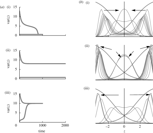
Figure 13 shows the behaviour near the threshold, for β = 4, θ = 0. The middle row shows the dynamics when coexistence is possible: a population that starts in linkage equilibrium maintains a unimodal distribution, whereas one that starts in strong linkage disequilibrium maintains its initial bimodal distribution. (At least, for 2000 generations, it is difficult to precisely determine stability.) For slightly lower genetic variance (top row), the peaks of an initially bimodal distribution gradually move together, as a result of gene flow from the opposite niche. For around 800 generations, the divergence suddenly collapses to give an approximately Gaussian distribution, with little divergence between niches. For slightly higher genetic variance (bottom row), the opposite is seen: an initially narrow unimodal distribution gradually broadens under disruptive selection, until two peaks emerge and diverge rapidly, greatly reducing gene flow.

Figure 13.

Behaviour near the threshold between unimodal and bimodal equilibria. (a) Shows the trait variance, across both niches, against time, starting either from complete linkage disequilibrium (LD, a(i)) or linkage equilibrium (LE, a(iii)). There are n = 40 loci, β = 4, and niches are of equal size. The standard deviation at linkage equilibrium is (a)(i)–(iii). (b) Shows the viabilities in each niche (thick curves; equation (2.3)), together with the trait distribution over successive generations. (i) , t = 100, 200, … , 1000, starting in LD; (ii) , t = 20, 40, … , 200, starting in LD and in LE; (iii) , t = 100, 200, … , 1000, starting in LE.

(c). Divergence in parapatry

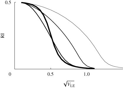
We have seen that sympatric speciation is possible if genetic variance in viability is higher than a threshold value, which decreases with the strength of disruptive selection, β (figure 11). Speciation should be easier if divergent populations, adapted to different niches, meet, since gene flow will increase linkage disequilibrium and facilitate divergence within a mixed habitat. Figure 14 shows that low levels of gene exchange with adjacent demes can greatly reduce the threshold for speciation. In a single population, reproductive isolation is almost complete if , for β = 2. However, if that population exchange a fraction m/2 of migrants from each of the two flanking demes, which contain only one or other niche, then the threshold is reduced, to approximately 1.0 for m = 0.02, and to approximately 0.7 for m = 0.2; a further increase to m = 0.5 has a smaller effect. (Note that even for the highest level of gene flow, the flanking demes remain divergent, and dominated by a single peak.)

Figure 14.

The effect of migration, m, on reproductive isolation. The chance that a survivor in one niche was born in a different niche (RI) is plotted against the standard deviation at linkage equilibrium , as in figure 11. Migration rate is m = 0, 0.02, 0.1, 0.5 (thin to thick lines). The focal deme exchanges a fraction m/2 of individuals with each of two flanking demes; one has only niche 0, and the other, only niche 1. β = 2, n = 40 loci; otherwise, parameters as in figure 9.

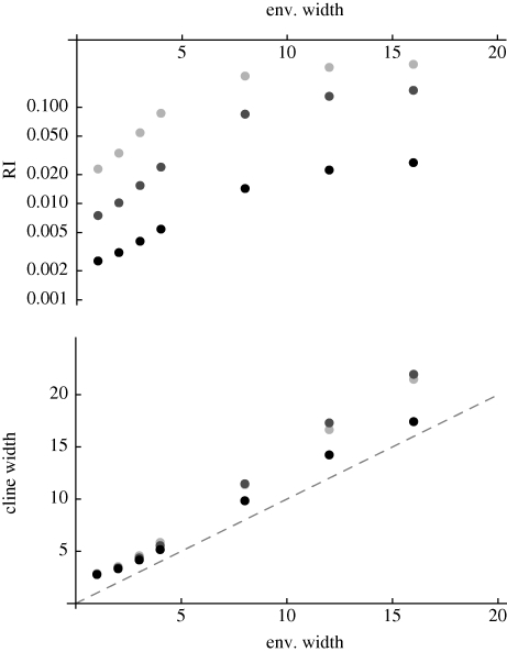
What happens across a broad one-dimensional cline in niche abundance, c_i? If niche size changes over a much longer spatial scale than dispersal, then gene flow will have a negligible effect, and each local population will reach an equilibrium, determined by the local environment (figure 7). If the niche abundance changes more sharply, then gene flow will generate additional genetic variance and is expected to increase the degree of reproductive isolation. Figure 15a illustrates this point, by showing how the strength of reproductive isolation in the central deme increases, as the cline becomes sharper. However, because selection towards the local equilibrium is strong, gene flow does not have an overwhelming effect: the width of the cline in trait mean is always close to the width in niche size (figure 15a).

Figure 15.

Effect of gene flow across a linear cline. Niche size, c₁, changes across a cline of 40 demes, in a logistic curve with width (defines as 1/max. gradient) plotted on the horizontal axis. (a) Shows the chance that an individual niche 1 in the central deme was born in niche 0 (regardless of spatial location). (b) Shows the width of the cline in trait mean; the dashed curve indicates the line where the two widths are equal. β = 2, θ = 0, 20 loci; (black to light grey).

In the narrow parameter regime where alternative stable equilibria coexist, gene flow can increase the genetic variance enough to trigger a transition to broad sympatry. A shallow cline in niche size (or any factor that causes geographic divergence) can increase genetic variance enough that the population at the centre establishes a bimodal distribution; this then spreads out to cover the entire range (figure 16). Here, parameters are such that in a single population, a unimodal distribution would be stable over a wide range of niche abundance. However, a sharp step in niche size at the centre of a linear cline causes an increase in variance and triggers a shift to the alternative bimodal distribution at the centre; this propagates outwards at a steady speed. The trait mean does not change much (figure 16a), since in both states the mean matches the environment. However, the variance increases drastically (figure 16b).

Figure 16.

Speciation can be triggered by gene flow in parapatry. In this example, selection is in the narrow range in which alternative stable states are possible: β = 4, θ = 0, 0, n = 40 loci (figure 13, a(ii), b(ii)). The population is distributed on a linear cline of 60 demes, with migration between nearest neighbours at a rate m = 1/2; niche size varies along the cline, from 0.3 on the left to 0.7 on the right, in a logistic curve with width 1 (black curve at (a)). Initially, the population is at linkage equilibrium with equal allele frequencies. (a) Shows the allele frequency clines at t = 0, 200, … , 2000 generations; (b) shows the clines in trait variance, over the same intervals.

Random fluctuations could cause a similar sudden transition from one species to the other, even in a homogeneous environment. However, as noted above, unless disruptive selection is extremely strong (β ≫ 1, θ ∼ 0, n ≫ 1), alternative equilibria can only coexist for a narrow parameter range. Typically, there is a single globally stable equilibrium, and the outcome is determined primarily by the local environment.

5. Discussion

Selection must necessarily be involved in speciation: reproductive isolation is defined by selection against hybrids; evolution of sympatry requires adaptation to, and choice of, different limiting resources; and selection may be responsible for most of the changes that lead incidentally to isolation. However, the key questions concern the interaction between selection and gene flow. Can selection overcome gene flow, allowing divergence in parapatry or even sympatry? When can selection favour reproductive isolation as an adaptation to reduce gene flow? How can coexistence in sympatry be achieved?

To begin to answer such questions, I analyse the Levene model, in which individuals settle in one of the two niches according to their genotype, and each niche contributes a fixed proportion to the whole population. Although this model has been widely used as the basis for simulations of sympatric speciation, it has hardly yet been analysed in depth (see Gavrilets 2004 for a review). We have concentrated on the case most favourable to speciation, where mating occurs randomly within niches. Thus, habitat preference is a ‘magic trait’ that causes reproductive isolation as well as exploitation of a particular niche.

A pure habitat preference does not alter overall genotype frequencies, but simply moves genotypes to different niches. Therefore, allele frequencies evolve neutrally, apart from the constraint that the proportion settling in a niche should match the contribution of that niche. Remarkably, if mating occurs within niches, then populations evolve to pairwise linkage equilibrium within those niches, regardless of the genetic basis of habitat preference or of the pattern of recombination. With a moderately large number of loci and an additive preference trait, there is a Gaussian trait distribution within each niche. The degree of divergence between niches depends on the underlying genetic variance: if this is high, there can be strong reproductive isolation. However, isolation varies smoothly with the genetic variance and can readily increase or decrease (figure 11, right).

If there is a concave trade-off between viabilities in the two niches, then disruptive selection favours maximum genetic variance, but is opposed by recombination. Now, there is a sharp threshold between unimodal and bimodal distributions, i.e. between one species and two (figure 11, left). Nevertheless, there is typically only a single global equilibrium: if the genetic variance is below some threshold, a bimodal distribution will collapse through introgression, while conversely, if it is above the threshold, an initially well-mixed population will split into two. These alternative states can only be simultaneously stable if there are many loci, and disruptive selection is strong (figure 13).

An unexpected result from this analysis is the key role played by the survival of an extreme specialist in the ‘wrong’ niche, denoted by θ. If this is appreciable, then it is possible for a sexual population to fix for one or the other specialist; otherwise, for θ = 0, a sexual population with low variance always evolves an intermediate generalist phenotype. Moreover, appreciable survival in the ‘wrong’ niche greatly reduces the reproductive isolation that can be achieved, even when an intermediate state is stable (figure 12). Sympatric speciation only seems possible when specialists do very badly in the wrong place.

I have not explicitly modelled the coupling between preference and trait that would be expected to evolve, strengthening reproductive isolation. This coupling was emphasized by Felsenstein (1981) in his ‘two-allele’ model, and analysed more generally by Barton & de Cara (2009). However, the analysis given here does deal with the coupling between preference alleles or between viability alleles, which inflates genetic variance and so can trigger speciation. Moreover, a coupling between preference and viability is implicit in the analysis. All that matters for the population genetics is the product of these two, α_γv_γ. The separate constraints on each can be combined into a joint constraint, which is necessarily concave (equation (3.1)). Thus, if we think of the underlying trait space (a, z), we can imagine two axes—one, along the trade-off curve, and one transverse to it. Since selection pushes the population onto the trade-off curve, we can follow evolution along it as if following a single trait. This argument suggests that the single-trait analysis given here will extend much more generally, at least qualitatively.

Whether speciation occurs in a single population depends primarily on the underlying genetic variance. Thus, gene flow from divergent populations can greatly facilitate speciation, by inflating the variance. Even low levels of migration can have a large effect, suggesting that speciation will be much easier in parapatry, with heterogeneity in niche size from place to place (figure 14).

Mallet et al. (2009) have argued that even when there is appreciable spatial subdivision on a fine scale, the distribution should still be referred to as ‘sympatric’ (or perhaps, as ‘mosaic sympatry’). In response, Fitzpatrick et al. (2009) argue for retaining the strict population genetic definition of sympatry, where the probability of mating must depend solely on genotype and not on birthplace. We agree with this latter view, at least for discussion of the population genetics of speciation. The real issue is whether selection causes changes that lead only incidentally to speciation or whether instead it acts directly to reduce gene exchange. On the one hand, mechanisms for allopatric divergence all extend to parapatry and operate in the presence of some gene flow; yet, they retain their essential character of leading to isolation only as a side effect. Conversely, mechanisms of sympatric speciation, involving selection for modifiers that increase isolation, or for association between alleles that increase it (i.e. one- or two-allele models; Felsenstein 1981), will also operate in parapatry and, usually, more effectively. It seems clearest to analyse first the extreme cases of strict allopatry or sympatry, and then to find how plausible these are in the more realistic care of parapatry—whether modelled as discrete demes or a spatial continuum.

The analysis given here is only preliminary, but does lay out a framework for future work. It should be extended beyond the logistic model (equations (2.3) and (2.4)), to find more generally when there is a sharp threshold for isolation, and when alternative states can coexist, allowing for the possibility of a sudden transition to sympatry (figure 16). The coupling between preference and viability needs to be modelled explicitly, and related to the single-trait analysis. The results here suggest that much can be captured by the infinitesimal model, a promising way to avoid the complexities of detailed genetics. Hopefully, this first effort will encourage future, more detailed, analyses of speciation.

Appendix A. Multilocus analysis

This section gives general expressions for the effects of selection and habitat preference in the two-niche Levene model. With habitat preference alone, this analysis shows that, on average, there is zero pairwise linkage equilibrium within niches.

(a). Multilocus notation

We follow the notation of Kirkpatrick et al. (2002). All loci are assumed to carry two alleles, labelled by X_i = 0 or 1. Overall allele frequencies, p_i, are assumed to stay constant, so that they can be used as a fixed reference point against which to define linkage disequilibria. Thus, the association among the set U of alleles is defined as D_U = E[ζ_U], where ζ_U ≡ . Here, the expectation is over the population of newborn haploid individuals; associations within niche γ are denoted by D_γ;U = E_γ[ζ_U], taking the expectation over genotypes within that niche. By definition, D_i = 0 in the population as a whole, but D_γ;i gives the change in allele frequency within niche γ.

To find changes in allele frequencies and linkage disequilibria, we must write the relative fitness within niche γ as a sum involving selection coefficients a_γ;U on sets of alleles Y:

A1

where the sum is over all subsets of the set of selected loci Ω. If the survivors from each niche mix into a common pool of mates, then all that matters is the selection coefficient, averaged over niches. Immediately after selection, but before random mating, recombination and mixing across niches, selection changes the linkage disequilibria in niche γ to

A2

Assuming that random mating and recombination occur within niches, we find that after recombination, the linkage disequilibria among the set of alleles U are given by a sum over the rates r_S,T at which recombination brings together sets S,T of loci to make up the set ST = U. D_γ;U^* = ∑_ST=U r_S,T D_γ;S D_γ;S. Finally, after mixing across niches:

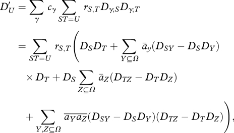A3

where = ∑_γc_γa_γ;Y, = ∑_γ c_γa_γ;Y a_γ;Z.

Note that the last term, involving the covariance of selection coefficients across niches, , will contribute even if there is no net selection, , averaged over niches. However, if mixing occurs before random mating across the whole population, then this last term does not appear.

The net change in allele frequencies is obtained by setting U = i in equation (A 3):

A4

Since we assume equilibrium, this must be zero for all loci, i. This constraint will be satisfied if there is no net selection on any set of loci (ā_y = 0 ∀ Y). However, there may also be equilibria where directional selection (∼ā_iD_ii = ā_ip_iq_i) is balanced by epistatic selection (∼ā_jkD_ijk).

The pairwise disequilibria are obtained by setting U = ij in equation (A 3):

A5

Again, the last term must be dropped if mixing occurs before meiosis. We see that at equilibrium

A6

The first term represents the generation of disequilibria by epistatic selection; when selection is weak, the leading term is ā_ijp_iq_ip_jq_j. The second term is due to mixing between niches, followed by recombination. At equilibrium, its contribution is independent of r_i,j, because recombination both generates and breaks up the association. With weak selection, it approximately equals p_iq_ip_jq_j. This last term must be dropped if mixing occurs before meiosis.

The analogous expression for three loci is the sum of three components, from the three distinct kinds of recombination event. Thus, in contrast to pairwise associations, the disequilibria due to mixing across niches are no longer independent of the recombination rates.

(b). Habitat preference

If there is variation solely in habitat preference (i.e. v_γ = 1 for all genotypes), then we have the strong constraint that every individual must go somewhere: ∑_γ α_γ(X) = 1 ∀ X. Thus, equation (A 1) implies that and . At the ESS for preference, the mean preference matches the output from each niche, and so . Then, the constraint that preferences sum to 1 implies that there is no net selection: . This is obvious, since at the ESS, all genotypes have the same fitness, so that preference is neutral. If mating occurs after mixing, in the population as a whole, then linkage disequilibria tend to zero under recombination alone. However, if mating and meiosis occur within niches, the subsequent mixing will generate linkage disequilibria. From equation (A 6), ∑_Y,Z⊆Ω D_iYD_jZ. With two niches, and the constraint that at ESS, we can simplify by writing a_0;Y = −c₁A_Y, a_1;Y = c₀A_Y, so that = c₀c₁A_YA_Z. Here, Δ_Y is a measure of the component of the difference in preference between niches that is due to the set of loci Y. With this definition, at equilibrium, the linkage disequilibrium is the product of two quantities:

A7

where Δ_U ≡ ∑_Y⊆Ω A_Y(D_UY − D_UD_Y).

Δ_U is the total divergence between niches D_1;U − D_0;U that is caused by selection.

For pairwise associations, the equilibrium is independent of recombination:

A8

This is precisely the pairwise linkage disequilibrium that would be produced by mixing two populations that differ in allele frequency by Δ_i, Δ_j. Therefore, the average pairwise linkage disequilibrium within niches must be zero (c₀D_0,ij + c₁D_1,ij = 0). This is a very general result, which applies with any relation between genotype and preference; it would also apply to viability selection within niches, provided that there is a linear trade-off between viabilities in each niche (i.e. v₀ + v₁ = constant).

We can write the divergence at locus i, Δ_i, as the sum of a component due to selection on i, plus components due to selection on other loci, that is mediated by the corresponding linkage disequilibrium:

A9

Here, we have used the relation D_ii = p_iq_i, which applies with two alleles per locus. With weak preference, Δ_i ∼ p_iq_iA_i, and so D̂_ij ∼ c₀c₁p_iq_ip_jq_jA_iA_j; pairwise disequilibrium is generated mainly by the differences in allele frequency between niches. If selection acts mainly on allele frequencies (i.e. if A_Y is negligible for |Y| > 1), then we have a closed set of equations:

A10

which can be solved numerically, or by expanding in c₀ c₁:

A11

where .

References

- Barton N. H., de Cara M. A. R.2009The evolution of strong reproductive isolation. Evolution 63, 1171–1190 (doi:10.1111/j.1558-5646.2009.00622.x) [DOI] [PubMed] [Google Scholar]
- Barton N. H., Shpak M.2000The stability of symmetrical solutions to polygenic models. Theor. Popul. Biol. 57, 249–264 (doi:10.1006/tpbi.2000.1455) [DOI] [PubMed] [Google Scholar]
- Bateson W.1909Heredity and variation in modern lights. In Darwin and modern science (ed. Seward A. C.), pp. 85–101 Cambridge, UK: Cambridge University Press [Google Scholar]
- Bomblies K., Weigel D.2010Arabidopsis and relatives as models for the study of genetic and genomic incompatibilities. Phil. Trans. R. Soc. B 365, 1815–1823 (doi:10.1098/rstb.2009.0304) [DOI] [PMC free article] [PubMed] [Google Scholar]
- Bürger R.In press Evolution and polymorphism in the multilocus Levene model without epistasis. Theor. Popul. Biol. [DOI] [PMC free article] [PubMed] [Google Scholar]
- Carson H. L., Templeton A. R.1984Genetic revolutions in relation to speciation phenomena: the founding of new populations. Annu. Rev. Ecol. Syst. 15, 97–131 (doi:10.1146/annurev.es.15.110184.000525) [Google Scholar]
- Cronin H.1991The ant and the peacock: altruism and sexual selection from Darwin to today Cambridge, UK: Cambridge University Press [Google Scholar]
- Darwin C.1859On the origin of species by means of natural selection London, UK: John Murray [Google Scholar]
- Diehl S. R., Bush G. L.1989The role of habitat preference in adaptation and speciation. In Speciation and its consequences (eds Otte D., Endler J. A.), pp. 345–365 Sunderland, MA: Sinauer Press [Google Scholar]
- Dobzhansky T.1937Genetics and the origin of species New York, NY: Columbia University Press [Google Scholar]
- Dobzhansky T.1940Speciation as a stage in evolutionary divergence. Am. Nat. 74, 312–321 (doi:10.1086/280899) [Google Scholar]
- Felsenstein J.1981Skepticism towards Santa Rosalia, or why are there so few kinds of animals? Evolution 35, 124–138 (doi:10.2307/2407946) [DOI] [PubMed] [Google Scholar]
- Fitzpatrick B. M., Fordyce J. A., Gavrilets S.2009Pattern, process and geographic modes of speciation. J. Evol. Biol. 22, 2342–2347 (doi:10.1111/j.1420-9101.2009.01833.x) [DOI] [PubMed] [Google Scholar]
- Gavrilets S.2004Fitness landscapes and the origin of species Princeton, NJ: Princeton University Press [Google Scholar]
- Gavrilets S., Gravner J.1997Percolation on the fitness hypercube and the evolution of reproductive isolation. J. Theor. Biol. 184, 51–64 (doi:10.1006/jtbi.1996.0242) [DOI] [PubMed] [Google Scholar]
- Geritz S. A. H., Kisdi E.2000Adaptive dynamics in diploid, sexual populations and the evolution of reproductive isolation. Proc. R. Soc. Lond. B 267, 1671–1678 (doi:10.1098/rspb.2000.1194) [DOI] [PMC free article] [PubMed] [Google Scholar]
- Geritz S. A. H., Kisdi E., Meszena G., Metz J. A. J.1998Evolutionarily singular strategies and the adaptive growth and branching of the evolutionary tree. Evol. Ecol 12, 35–57 (doi:10.1023/A:1006554906681) [Google Scholar]
- Huxley T. H.1860The origin of species. Westminster Rev. 17, 541–560 [Google Scholar]
- Innan H., Stephan W.2001Selection intensity against deleterious mutations in RNA secondary structures and rate of compensatory nucleotide substitutions. Genetics 159, 389–399 [DOI] [PMC free article] [PubMed] [Google Scholar]
- Kirkpatrick M., Barton N. H.2006Chromosome inversions, local adaptation, and speciation. Genetics 173, 419–434 (doi:10.1534/genetics.105.047985) [DOI] [PMC free article] [PubMed] [Google Scholar]
- Kirkpatrick M., Johnson T., Barton N. H.2002General models of multilocus evolution. Genetics 161, 1727–1750 [DOI] [PMC free article] [PubMed] [Google Scholar]
- Kondrashov A. S.2002Accumulation of Dobzhansky-Muller incompatibilities within a spatially structured population. Evolution 57, 151–153 [DOI] [PubMed] [Google Scholar]
- Levene H.1953Genetic equilibrium when more than one niche is available. Am. Nat. 87, 331–333 (doi:10.1086/281792) [Google Scholar]
- Levins R.1968Evolution in changing environments Princeton, NJ: Princeton University Press [Google Scholar]
- Mallet J., Meyer A., Nosil P., Feder J. L.2009Space, sympatry and speciation. J. Evol. Biol. 22, 2332–2341 (doi:10.1111/j.1420-9101.2009.01816.x) [DOI] [PubMed] [Google Scholar]
- Maynard Smith J.1966Sympatric speciation. Am. Nat. 100, 637–650 (doi:10.1086/282457) [Google Scholar]
- Maynard Smith J., Hoekstra R.1980Polymorphism in a varied environment—how robust are the models ? Genet. Res. 35 45–57 (doi:10.1017/S0016672300013926) [DOI] [PubMed] [Google Scholar]
- Mayr E.1963Animal species and evolution. Cambridge, MA: Harvard University Press [Google Scholar]
- Muller H. J.1942Isolating mechanisms, evolution and temperature. Biol. Symp. 6, 71–125 [Google Scholar]
- Nagylaki T.2009Evolution under the multilocus Levene model without epistasis. Theor. Popul. Biol. 76, 197–213 (doi:10.1016/j.tpb.2009.07.003) [DOI] [PubMed] [Google Scholar]
- Navarro A., Barton N. H.2003Accumulating postzygotic isolation genes in parapatry: a new twist on chromosomal speciation. Evolution 57, 447–459 [DOI] [PubMed] [Google Scholar]
- Orr H. A.1995The population genetics of speciation: the evolution of hybrid incompatibilities. Genetics 139, 1805–1813 [DOI] [PMC free article] [PubMed] [Google Scholar]
- Orr H. A.1996Dobzhansky, Bateson and the genetics of speciation. Genetics 144, 1331–1335 [DOI] [PMC free article] [PubMed] [Google Scholar]
- Orr H. A., Presgraves D. C.2000Speciation by postzygotic isolation: forces, genes and molecules. BioEssays 22, 1085–1094 (doi:10.1002/1521-1878(200012)22:12) [DOI] [PubMed] [Google Scholar]
- Orr H. A., Turelli M.2001The evolution of postzygotic isolation: accumulating Dobzhansky–Muller incompatibilities. Evolution 55, 1085–1094 [DOI] [PubMed] [Google Scholar]
- Patton J. L., Sherwood S. W.1983Chromosome evolution and speciation in rodents. Annu. Rev. Syst. Ecol. 14, 139–158 [Google Scholar]
- Poulton E. B.1903What is a species? Proc. Entomol. Soc. Lond. 1903, xxvii–cxvi [Google Scholar]
- Searle J. B.1993Chromosomal hybrid zones in eutherian mammals. In Hybrid zones and the evolutionary process (ed. Harrison R. G.), pp. 309–353 Oxford, UK: Oxford University Press [Google Scholar]
- Servedio M. R., Noor M. A.2003The role of reinforcement in speciation: theory and data. Annu. Rev. Ecol. Syst. 34, 339–364 (doi:10.1146/annurev.ecolsys.34.011802.132412) [Google Scholar]
- Slatkin M.1973Gene flow and selection in a cline. Genetics 75, 733–756 [DOI] [PMC free article] [PubMed] [Google Scholar]
- Udovic D.1980Frequency-dependent selection, disruptive selection, and the evolution of reproductive isolation. Am. Nat. 116, 621–641 (doi:10.1086/283654) [Google Scholar]
- Wallace A. R.1889Darwinism London, UK: Macmillan [Google Scholar]
- White M. J. D.1978Modes of speciation San Francisco, CA: WH Freeman [Google Scholar]
- Wright S.1932The roles of mutation, inbreeding, crossbreeding and selection in evolution. Proc. Sixth Int. Congress in Genetics, Ithaca, NY, 1932, vol. 1, pp. 356–366 Menasha, WI: Brooklyn Botanic Garden [Google Scholar]
- Wright S.1941On the probability of fixation of reciprocal translocations. Am. Nat. 75, 513–522 (doi:10.1086/280996) [Google Scholar]