Model-Based Estimation of Ventricular Deformation in the Cat Brain

Abstract

The estimation of ventricular deformation has important clinical implications related to neuro-structural disorders such as hydrocephalus. In this paper, a poroelastic model was used to represent deformation effects resulting from the ventricular system and was studied in 5 feline experiments. Chronic or acute hydrocephalus was induced by injection of kaolin into the cisterna magna or saline into the ventricles; a catheter was then inserted in the lateral ventricle to drain the fluid out of the brain. The measured displacement data which was extracted from pre-drainage and post-drainage MR images were incorporated into the model through the Adjoint Equations Method. The results indicate that the computational model of the brain and ventricular system captured 33% of the ventricle deformation on average and the model-predicted intraventricular pressure was accurate to 90% of the recorded value during the chronic hydrocephalus experiments.

1 Introduction

The cerebral ventricles in the brain are cavities filled with cerebrospinal fluid (CSF). The deformation of the ventricular system is related to diseases such as hydrocephalus and edema but may also occur as the result of a space occupying lesion. Together with the compression of the white matter adjacent to the ventricles, these diseases can cause serious neurological problems including cognitive impairment and even death.

Different research groups have been studying the mathematical modeling of the ventricular system in the brain. Drake’s approach represents the brain as a lumped-parameter system [1], but given that the brain is a sponge-like material, a more realistic poroelastic model has been investigated to incorporate the fluid distribution in the parenchyma. Nagashima et al. [2] modeled the brain and ventricles based on Biot’s consolidation theory [3]. A 2D finite element model of the parenchyma was created using computed tomography (CT) scans. Pena et al. further studied the poroelastic model to represent the stress concentrations and ventricular anatomy more accurately [4, 5]. Several groups have attempted to improve the boundary conditions and material parameters used in the poroelastic model [6, 7, 8]. Miller et al. proposed a nonlinear viscoelastic representation [9]. Kyriacou et al. compared it with the linearly elastic approach and concluded that the viscoelastic model is more suitable to capturing high stain rates [10]. Considering the fact that ventricular deformation is related to CSF flow and is not representative of high stain rate deformation, we modeled the brain as an elastic porous medium to allow the flow of the interstitial fluid into and out of the extracellular space through the ventricular walls. We represented the ventricular system through mixed boundary conditions and used sparse measurement data to estimate the driving fluid pressure required to deform the brain during the induction and release of pressure-induced ventriculomegaly. The importance of the work is that we show for the first time an algorithm that is able to successfully estimate the unknown pressure parameters in the boundary conditions from displacement data that allows the fluid-filled ventricles to be represented by their surface, rather than directly including them within the discretized computational domain in which case a phase change would need to be incorporated into the mechanical equations describing brain deformation that is far more complicated to implement numerically.

2 Materials and Methods

2.1 Experimental System

A group of five felines was studied with MR imaging for in vivo observation of the progression of ventricle deformation. Chronic or acute hydrocephalus was first induced by injection of kaolin into the cisterna magna or saline into the ventricle as a control. Following that, a catheter was inserted into the lateral ventricle to drain fluid out of the brain, which caused the enlarged ventricles to shrink. The model simulated the ventricular shrinking process.

Five adult female domestic felines were quarantined for three days prior to the beginning of the experiment. On the day of cisternal injection, general anesthesia was induced and a peripheral intravenous catheter was placed. All animals underwent baseline magnetic resonance imaging (MRI) of the brain. Animals then underwent cisternal injection of kaolin or saline. Each animal was placed prone on a heated operating table with the neck partially flexed. A pediatric spinal needle was inserted in the midline, under fluoroscopic guidance, into the occiput-C1 interspace until clear CSF was returned (Figure 1, left). The needle was secured using a mobile clamp affixed to the table (Figure 1, right). The kaolin dose was 10–50 mg mixed in sterile saline. Slow injection of kaolin was completed over 10 minutes.

Fig. 1.

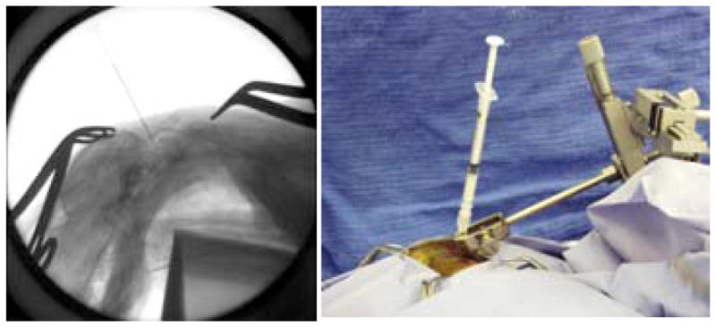
Lateral fluoroscopic view of injection via occiput-C1 interspace (left) and operative photograph of 1 cc syringe affixed to stabilizing clamp (right) [11]

Once ventriculomegaly was confirmed, a ventricular catheter connected to a subcutaneous reservoir was placed in the right frontal region, to enable subsequent measurement of intracranial pressure (ICP). The catheter-reservoir construct was inserted into the right lateral ventricle using a central stylet. [11]

Another MRI session was scheduled between 7 and 17 days after the initial injection. Cats were anesthetized and the animal’s head was fixed on the exam table as shown in Figure 2(a). After the ventricles were enlarged, a series of MR images were taken (Figure 2(b)). These images are referred to as pre-drainage MR. Intraventricular pressures (IVP) were measured after induction of hydrocephalus. One hour later, the fluid was drained out of the ventricle through the catheter. The enlarged ventricle shrunk markedly. Another set of images (Figure 2(c)) were acquired at this point which are called post-drainage MR. IVPs were measured again at this stage.

Fig. 2.

(a) The cat was anesthetized and the head was fixed on the exam table. (b) Pre-drainage MR. (c) Post-drainage MR of the same cat brain.

By comparing the two sets of images, substantial ventricular shrinkage was observed. We attempted to drain the ventricles in stages, for example, by removing fluid in 0.5 cc increments but observed a threshold effect whereby either no observable deformation occurred (if too little fluid was removed) or no additional deformation resulted (if more fluid was removed after an initial amount sufficient to cause an immediate and measurable reduction in ventricular size was taken). The images were acquired with a 3.0 T MRI (Philips) system and had a resolution of 256× 256 × 24 voxels and a voxel size of 0.3125 mm× 0.3125 mm× 1.2 mm.

2.2 Computational Model

The biomechanical model was based on Biot’s consolidation theory, and the brain was modeled as poroelastic material [3, 12]. The mathematical description is [13, 14]:

$$\begin{array}{l}\nabla ·G\nabla \text{u}+\nabla \frac{G}{1-2v}(\nabla ·\text{u})-\alpha \nabla p=\text{f}\\ \alpha \frac{\partial }{\partial t}(\nabla ·\text{u})+\frac{1}{S}\frac{\partial p}{\partial t}-\nabla ·k\nabla p=\mathrm{\Psi }\end{array}$$ (1)

where

• f body force (e.g., gravity) per unit volume (N/m³);

• Ψ pressure source strength (Pa/s);

• G shear modulus (Pa);

• v Poisson’s ratio;

  u displacement vector (m);

• p pore fluid pressure (Pa);

• α ratio of fluid vol. extracted to vol. change of the tissue under compression;

  k hydraulic conductivity (m³s/kg);

• 1/S amount of fluid which can be forced into the tissue under constant vol. (1/Pa).

By using the finite element method (FEM), these equations can be solved with the adjoint equations method (AEM) [15] to incorporate the intraoperative measurements.

2.3 Model Generation

The FEM discretization process begins with segmentation of the region of interest. A semi-automatic method was used to segment the cat brain and ventricles from the pre-drainage MR images. A surface description consisting of triangular patches was generated from the segmented brain and ventricles. Then, a 3-D tetrahedral mesh was created to define the computational domain. The volume mesh contained about 11,000 nodes and 53,000 elements. Given the boundary conditions and material properties, and the input of measured displacement data around the ventricle, the biomechanical model can be solved with FEM. The original mesh was deformed using the displacement results and the pre-drainage MR images were morphed to predict the post-drainage MR status. Figure 3 illustrates the entire procedure.

Fig. 3.

Illustration of the modeling procedure for the ventricular system in the brain

The ventricles were modeled as a cavity since they only include CSF which is treated as a void in the consolidation equations. Approximate boundary conditions were imposed to simulate the physical conditions. The upper brain surface was specified as stress free and allowed free flow of CSF. The ventricle surface was set to be stress free to allow displacements, and pressure was handled by a mixed (type 3) boundary condition, $\frac{\partial p}{\partial n}=k(p-p_v)$ where p is the brain tissue interstitial pressure, n is the normal to the boundary of the ventricle, p_v is the ventricle fluid pressure and k is the conductivity coefficient. This condition specifies the drainage through the ventricle surface as a function of the interstitial pressure and permeability of the ventricular wall. The flow of fluid is determined by the hydraulic conductivity and the pressure difference between the interstitial and ventricular fluid pressures. The lower part of the brain was modeled as brainstem which was assumed to have no displacements and free flow of CSF.

Reliable tissue properties are important to the biomechanical modeling. There are many studies on the mechanical properties of brain tissue. The material properties deployed here were Young’s modulus E = 3240 Pa, Poisson’s ratio v = 0.45 and the hydraulic conductivity, k = 1× 10⁻⁷m³s/kg [14, 16].

3 Results

The first cat was a control animal. Saline was infused into the ventricle before the pre-drainage stage of the experiment. Fluid was drained from the ventricle before the post-drainage MR session. In Figure 4(a), the red arrows around the ventricles show the 31 sparse data points which were incorporated into the model. They were evenly distributed around the ventricles, except in areas where unreliable displacements were measured. In the quantitative validation, the number of validation data points was 1105. The brain configuration and ventricle deformation are presented in Figure 4(b), which shows that the maximum displacement is about 3 mm. In Figure 4(c), the gray color is the pre-drainage ventricle, the brown color is the measured post-drainage ventricular shape (after shrinkage), and the green is the model estimate of the post-drainage ventricle. The 3D view shows that the model results match the measured ones very well. In order to better visualize the model results, four 2D slices were generated to produce an overlay of the ventricle boundary in the 3 experimental states.

Fig. 4.

(a) Sparse data distribution around the ventricle used for data assimilation in cat 1. (b) Displacement results of the cat brain surface. (c) Overlay of the pre-drainage ventricle (gray), post-drainage ventricle (brown) and model estimated post drainage ventricle (green).

In Figure 5 (left), the blue line is the pre-drainage ventricle, background MR shows the post-drainage ventricle, and the red dots represent the model estimate of the post-drainage ventricle. The pre-drainage ventricle (blue) is large as seen from the 2D slices. After the fluid was drained, its size shrunk. The model result (red) matches the measurement (MR) better in the slices compared to the pre-drainage ventricle (blue).

Fig. 5.

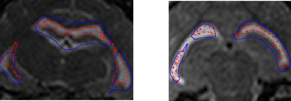
Overlays of the predrainage ventricle (blue), postdrainage ventricle (background MR) and model deformed ventricle (red) for cat 1(left) and cat 2 (right)

The second cat was also a control animal. There were 48 sparse data around the ventricle used in this case and 710 data were deployed for validation. The results are shown in Figure 5 right. The 2D overlay indicates the model made certain improvements for cat 2. For both of the control animals, the model-estimated intraventricular pressure was less than 1000 Pa, which is lower than the measured 3000 Pa pressure. This may have occurred because of the leakage of fluid around the catheter, an effect which was observed during the injection in the experiments. Another possible explanation is that the fluid can flow out the lateral ventricle through the third ventricle, and therefore, reduce the pressure around the lateral ventricles which are modeled in the study.

The remaining three cats underwent hydrocephalus experiments. Hydrocephalus was induced by injection of kaolin into the cisterna magna. The intraventricular pressure was different in the pre-drainage state, but it was the same post-drainage and equaled 500 Pa. The difference in the measured intraventricular pressure between the two stages was 1000 Pa, 700 Pa and 600 Pa for cat 3, cat 4 and cat 5, respectively.

The displacement results for cat 3, cat 4 and cat 5 are reported in Figure 6 left, middle and right, respectively. The number of sparse data was 35, 31 and 41 and number of validation points was 414, 381 and 719 in each case, respectively. Points were evenly distributed around the ventricle. The model estimations achieved different levels of success. Both the displacement and pressure results from the model match the measurements. The model estimations of IVP were 900Pa, 730Pa and 570 Pa, respectively. Compared to the measured pressure differences of 1000 Pa, 700 Pa and 600 Pa, the model estimates were accurate to 90% in all three experiments.

Fig. 6.

Overlays of the pre-drainage ventricle (blue), post-drainage ventricle (background MR) and model deformed ventricle (red) for cat 3 (left), cat 4 (middle) and cat 5 (right)

A quantitative comparison of the displacement results is shown in Table 1. The data indicates that in all five cases, the model captured 33% of the deformation on average. The misfit reported in Table 1 is the average distance between the measured and model estimated ventricles for each cat.

Table 1.

The misfit before and after the model prediction for five cat studies

	Mean Misfit (before) (mm)	Mean Misfit (after) (mm)	Improvements (%)
Cat1	1.27	0.786	38.0
Cat2	0.799	0.555	30.5
Cat3	0.616	0.419	32.0
Cat4	0.515	0.349	32.8
Cat5	0.725	0.364	29.9

4 Discussion

The results showed that the computational method was able to estimate ventricular deformation in the cat brain within 1 mm through type 3 boundary condition representation of the ventricular surface which holds promise for improving modeling accuracy as well as avoiding the need of implementing the more complicated mechanical modeling framework that would be required to represent the fluid phase of the ventricles, if they are discretized directly within the computational domain. The quantitative analysis indicates that the model captured 33% of the ventricular deformation on average in five cat experiments and the model estimated IVP to be accurate within 90% compared to the measured value in the chronic hydrocephalus experiments.

Although the mathematical representation of the ventricles has produced relatively good results, in some respects the average percentage of deformation capture (33%) is disappointing. Here, it is important to recognize that the overall deformation in the cat brain was very small (~ 1mm), placing a premium on the fidelity of the image processing and displacement data extraction procedures that were used in the study. Further investigations are needed to explore the extent to which the modeling errors are, in part, a result of imperfections in the data analysis techniques. For example, in the segmentation and surface and volume meshing processes, error is accumulated and can be reduced. The nonrigid motion of the ventricles was also approximated through Iterative Closest Point to determine displacements. In order to provide better guidance and improve model-data mismatch, more accurate displacement measurements are needed. The brain mechanical properties employed in this study were taken from the literature whereas material properties determined experimentally for each feline brain will likely contribute to improved modeling accuracy.

The methodology can be extended to human clinical studies. Since the CSF pressure in the intraventricular space is measurable during the neurosurgery, data on both displacement and pressure will be available. The measurements can then be used as data for the model computed brain deformation. Incorporating the ventricle structure and the pressure data will help to further develop the model to yield more accurate estimates of the state of the brain during surgery and can help the surgeon to optimize the planned surgical path. Additional clinical studies are needed for future validation at the human scale but the in vivo results presented here in the cat brain appear promising and suggest that the approach will be successful in humans as well.

References

- 1.Drake J, Kestle J, Milner R. Randomized clinical trials of cerebrospinal fluid shunt design in pediatric hydrocephalus. Neurosurgery. 1998;43:294–305. doi: 10.1097/00006123-199808000-00068. [DOI] [PubMed] [Google Scholar]
- 2.Nagashima T, Tamaki N, Matsumoto S, Horwitz B, Seguchi Y. Biomechanics of hydrocephalus: a new theoretical model. Neurosurgery. 1987;21:898–903. doi: 10.1227/00006123-198712000-00019. [DOI] [PubMed] [Google Scholar]
- 3.Biot M. General theory of three-dimensional consolidation. Journal of Applied Physics. 1941;12:155–164. [Google Scholar]
- 4.Pena A, Bolton MD, Whitehouse H, Pickard JD. Effects of brain ventricular shape on periventricular biomechanics: a finite element analysis. Neurosurgery. 1999;45:107–118. doi: 10.1097/00006123-199907000-00026. [DOI] [PubMed] [Google Scholar]
- 5.Pena A, Harris NG, Bolton MD, Czosnyka M, Pickard JD. Communicating hydrocephalus: the biomechanics of progressive ventricular enlargement revisited. Acta Neurochir Suppl. 2002;81:59–63. doi: 10.1007/978-3-7091-6738-0_15. [DOI] [PubMed] [Google Scholar]
- 6.Kaczmarek M, Subramaniam R, Neff S. The hydromechanics of hydrocephalus: steady state solution for cylindrical geometry. Bull Math Biol. 1997;59:295–323. doi: 10.1007/BF02462005. [DOI] [PubMed] [Google Scholar]
- 7.Tenti G, Sivaloganathan S, Drake J. Brain biomechanics: steady-state consolidation theory of hydrocephalus. Can Appl Maths. 1998 [Google Scholar]
- 8.Taylor Z, Miller K. Reassessment of brain elasticity for analysis of biomechanisms of hydrocephalus. J Biomech. 2004;37:1263–1269. doi: 10.1016/j.jbiomech.2003.11.027. [DOI] [PubMed] [Google Scholar]
- 9.Miller K, Chinzei K. Constitutive modelling of brain tissue: experiment and theory. J Biomech. 1997;30:115–1121. doi: 10.1016/s0021-9290(97)00092-4. [DOI] [PubMed] [Google Scholar]
- 10.Kyriacou S, Mohamed A, Miller K, Neff S. Brain mechanics for neurosurgery: modeling issues. Biomech Mod Mechanobiol. 2002;1:151–164. doi: 10.1007/s10237-002-0013-0. [DOI] [PubMed] [Google Scholar]
- 11.Lollis S, Hoopes P, Bergeron J, Kane S, Paulsen K, Weaver J, Roberts D. Low-dose kaolin-induced feline hydrocephalus and feline ventriculostomy: An updated model. Protocol. 2007 doi: 10.3171/2009.5.peds0941. [DOI] [PMC free article] [PubMed] [Google Scholar]
- 12.Nagashima T, Tamaki N, Takada M, Tada Y. Formation and resolution of brain edema associated with brain tumors. A comprehensive theoretical model and clinical analysis. Acta Neurochirurgica Suppl. 1994;60:165–167. doi: 10.1007/978-3-7091-9334-1_44. [DOI] [PubMed] [Google Scholar]
- 13.Paulsen K, Miga M, Kennedy F, Hoopes P, Hartov A, Roberts D. A computational model for tracking subsurface tissue deformation during stereotactic neurosurgery. IEEE Transactions on Biomedical Engineering. 1999;46:213–225. doi: 10.1109/10.740884. [DOI] [PubMed] [Google Scholar]
- 14.Miga M. Phd thesis. Thayer School of Engineering, Dartmouth College; Hanover, NH: Sep, 1998. Development and Quantification of a 3D Brain Deformation Model for Model-Updataed Image-Guided Stereotactic Neurosurgery. [Google Scholar]
- 15.Lynch DR. Numerical Partial Differential Equations for Environmental Scientists and Engineers - A First Practical Course. 2. Springer; Heidelberg: 2004. [Google Scholar]
- 16.Chinzei K, Miller K. Compression of swine brain tissue; experiment in vitro. J Mech Eng Lab. 1996;50:19–28. [Google Scholar]