Neural imaging to track mental states while using an intelligent tutoring system

Abstract

Hemodynamic measures of brain activity can be used to interpret a student's mental state when they are interacting with an intelligent tutoring system. Functional magnetic resonance imaging (fMRI) data were collected while students worked with a tutoring system that taught an algebra isomorph. A cognitive model predicted the distribution of solution times from measures of problem complexity. Separately, a linear discriminant analysis used fMRI data to predict whether or not students were engaged in problem solving. A hidden Markov algorithm merged these two sources of information to predict the mental states of students during problem-solving episodes. The algorithm was trained on data from 1 day of interaction and tested with data from a later day. In terms of predicting what state a student was in during a 2-s period, the algorithm achieved 87% accuracy on the training data and 83% accuracy on the test data. The results illustrate the importance of integrating the bottom-up information from imaging data with the top-down information from a cognitive model.

This article reports a study of the potential of using neural imaging to facilitate student modeling in intelligent tutoring systems, which have proven to be effective in improving mathematical problem solving (1, 2). The basic mode of operation of these systems is to track students as they solve problems and offer instruction based on this tracking. These tutors individualize instruction by two processes, called “model tracing” and “knowledge tracing.” Model tracing uses a model of students’ problem solving to interpret their actions. It tries to diagnose the student's intentions by finding a path of cognitive actions that match the observed behavior of the student. Given such a match, the tutoring system is able to provide real-time instruction individualized to where that student is in the problem. The second process, knowledge tracing, attempts to infer a student's level of mastery of targeted skills and selects new problems and instruction suited to that student's knowledge state. Although the principle of individualizing instruction to a particular student holds great promise, the practice is limited by the ability to diagnose what the student is thinking. The only information available to a typical tutoring system comes from the actions that students take in the computer interface. Inferences based on such impoverished data are tenuous at best, and brain imaging data might provide a useful augmentation. Recent research has reported a variety of successes in using brain imaging to identify what a person is thinking about (e.g., refs. 3 –6) and identifying when mental states happen (e.g., refs. 7 –9).

Although the methods described here could extend to knowledge tracing, this article will focus on model tracing where the goal is to identify the student's current mental state. Two features of the intelligent tutoring situation shaped our approach to the problem: (i) Given that instruction must be made available in real time, inferences about mental state can only use data up to the current point in time. Although inferences of mental state may become clearer after observing subsequent student behavior, these later data are unavailable for real-time prediction. (ii) Model tracing algorithms are parameterized with pilot data and then used to predict the mental state of students in learning situations. Therefore, we trained our algorithm on one set of data and tested it on a later set.

Although many distinctions can be made about mental states during the tutor interactions, we focused on two basic distinctions as a first assessment of the feasibility of the approach. The first distinction involved identifying periods of time when students were engaged in mathematical problem solving and periods of time when they were not. The second, more refined, distinction involved identifying what problem they were solving when they were engaged and where they were in the solution of that problem. One might think only the latter goal would be of instructional interest; however, detecting when students are engaged or disengaged during algebraic problem solving is by no means unimportant. A number of immediate applications exist for accurate diagnosis of student engagement. For example, there are often long periods when students do not perform any action with the computer. It would be useful to know whether the student was engaged in the mathematical problem solving during such periods or was off task. If the student was engaged in algebraic problem solving, despite lack of explicit progress, the tutor might volunteer help. On the other hand, if the student was not engaged, the tutoring system might nudge the student to go back on task.

The research reported here used an experimental tutoring system described in Anderson (10) and Brunstein et al. (11) that teaches a complete curriculum for solving linear equations based on the classic algebra text of Foerster (12). The tutoring system has a minimalist design to facilitate experimental control and detailed data collection: it presents instruction, provides help when requested, and flags errors during problem solving. In addition to teaching linear equations to children, this system can be used to teach rules for transforming data-flow graphs that are isomorphic to linear equations. The data-flow system has been used to study learning with either children or adults and has the virtue of not interfering with instruction or knowledge of algebra. The experiment reported here uses this data-flow isomorph with an adult population. Fig. 1 illustrates sequences of tutor interactions during a problem isomorphic to the simple linear equation x – 10 = 17. The interactions with the system are done with a mouse that selects parts of the problem on which to operate, actions from a menu, and enters values from a displayed keypad.

Fig. 1.

Sequences of tutor interaction during a problem isomorph. (A) The student starts out in a state with a data-flow equivalent of the equation x – 10 = 17. The student uses the mouse to select this equation and chooses the operation “Invert” from the menu. (B) A keypad comes up into which the student enters the result 17 + 10. (C) The transformation is complete. (D) The previous state (data-flow equivalent of x = 17 + 10) is repeated and the student selects 17 + 10 and chooses the operation “Evaluate”. (E) A keypad comes up into which the student will type “27.” (F) The evaluation is complete.

Results

Twelve students went through a full curriculum based on the sections in the Foerster text (12) for transforming and solving linear equations. The experiment spanned 6 days. On Day 0, students practiced evaluation and familiarized themselves with the interface. On Day 1, three critical sections were completed with functional magnetic resonance imaging (fMRI). On Days 2 to 4 more complex material was practiced outside of the fMRI scanner. On Day 5 the three critical sections (with new problems) were repeated, again in the fMRI scanner. Each section on Days 1 and 5 involved three blocks during which they would solve four to eight problems from the section. Some of the problems involved a single transformation-evaluation pair, as shown in Fig. 1, and others involved two pairs (problems studied on Days 2–4 could involve many more operations). Periods of enforced off-task time were created by inserting a one-back task (13) after both transformation and evaluation steps. A total of 104 imaging blocks were collected on Day 1 and 106 were collected on Day 5 from the same 12 students. Average time for completion of a block was 207 2-s scans with a range from 110 to 349 scans. The duration was determined both by the number and difficulty of the problems in a block and by the student's speed.

Student's solved 654 problems on Day 1 and 664 on Day 5. Of the problems, 76% on both days were solved with a perfect sequence of clicks. Most of the errors appeared to reflect interface slips and calculation errors rather than misconceptions. Each problem involved one or more of the following types of intervals:

• Transformation (steps A–C in Fig. 1): On Day 1 students averaged 8.2 scans, with a standard deviation of 5.9 scans. On Day 5 the mean duration was 5.9 scans, with a standard deviation of 4.1.

• One-back within a problem: This was controlled by the software and was always six scans.

• Evaluation (steps D–F in Fig. 1): Students took a mean of 4.9 scans on Day 1, with a standard deviation of 3.6; they took 3.8 scans on Day 5, with a standard deviation of 2.7.

• Between-problem transition: This involved six scans of one-back, a variable interval determined by how long it took students to click a button saying they were done, and two scans of a fixation cross before the next problem. This averaged 9.1 scans, with a standard deviation of 1.5 scans on both days.

In addition, there were two scans of a fixation cross before the first problem in a block and a number of scans at the end, which included a final one-back but also a highly variable period of 6 to 62 scans before the scanner stopped. The mean of this end period was 11 scans and the standard deviation was 6.5 scans.

The student-controlled transformation and evaluation intervals show a considerable range, varying from a minimum of 1 scan to a maximum of 54 scans. Anderson (10) and Anderson et al. (14) describe a cognitive model that explains much of this variance. For the current purpose of showing how to integrate a cognitive model and fMRI data, the complexity of that model would distract from the basic points. Therefore, we will adapt instead the keystroke model (15), based on the fact that cognitive complexity is often correlated with complexity in terms of physical actions. Such models can miss variability that is a result of more complex factors, but counting physical actions is often a good predictor.

We will use number of mouse clicks as our measure of complexity. As an example of the range in mouse clicks, it takes 15 clicks in the tutor interface to accomplish the following transformation:

but only 5 clicks to accomplish the evaluation:

For brevity we give the standard algebraic equivalent of data-flow graphs. The first example requires more clicks first to select parts of the problems to operate on and then to enter the more complex expressions (“1000/−10*” in one case versus “2” in the other case). Transformation steps take longer than evaluation steps because they require more clicks (average 10.4 clicks versus 6.8). Fig. 2 illustrates the systematic relationship that exists between mouse clicks required to accomplish an operation and the time that the operation took. The average scans per mouse click decreases from 0.77 scans on Day 1 to 0.57 on Day 5. On the other hand, the average ratio shows little difference between transformations (0.69 scans) and evaluations (0.65 scans), and so Fig. 2 is averaged over transformations and evaluations. As the figure illustrates, the number of scans for a given number of mouse clicks is approximately distributed as a log-normal distribution. Log-normal distributions estimated from Day 1 were part of the algorithm for identifying mental state. The only adjustment for Day 5 was to speed up the mean of the distribution by a constant 0.7 factor (based on ref. 10, figure 5.7) to reflect learning. Thus, the prediction for Day 5 is 0.77 × 0.7 = 0.54 scans per click.

Fig. 2.

Systematic relationship that exists between mouse clicks required to accomplish an operation and the time that the operation took. (A and C) The relationship between number of clicks and number of scans. (B and D) Distributions of number of scans for different numbers of clicks and log-normal distributions fitted to these.

Imaging Data.

Anderson et al. (14) describe an effort to relate fMRI activity in predefined brain regions to a cognitive model for this task. However, as with the latency data, the approach here makes minimal theoretical assumptions. As described in the Materials and Methods, we defined 408 regions of interest, each approximately a cube with sides of 1.3 cm that cover the entire brain. For each scan for each region, we calculated the percent change in the fMRI signal for that scan from a baseline defined as the average magnitude of all of the preceding scans in that block. We used this signal to identify “On” periods when a student was engaged in problem solving (evaluation and transformation in Fig. 1) versus “Off” periods when the student was engaged in n-back or other beginning and ending activities. A linear discriminant analysis was trained on the group data from Day 1 to classify the pattern of activity in the 408 regions as reflecting an On scan or an Off scan.

Fig. 3A shows how accuracy of classifying a target scan varied with the distance between the target scan and the scan whose activity was used to predict it. It plots a d-prime measure (16), which is calculated from the z-transforms of hit and false-alarm rates. Therefore, for example, using the activity two scans after the target scan, 91% of the 7,761 Day 5 On scans were correctly categorized and 16% of 11,835 Off scans were false alarmed, yielding a d-prime of 2.34. Fig. 3 shows that best prediction is obtained using activity two scans or 4 s after the target scan. Such a lag is to be expected given the 4- to 5-s delay in the hemodynamic response. The d-prime measure never goes down to 0, reflecting the residual statistical structure in the data. Although we will report on the results using a lag of 0, the main application will use the optimal lag-2 results, meaning it was 4 s behind the student.

Fig. 3.

Accuracy of classification and distribution of values. (A) Accuracy of classification as a function of the offset between the scan whose activity is being used and the scan whose state is being predicted. (B) Distribution of values for Day 1 and Day 5 On and Off scans using an offset of 2. All 408 regions are used.

Little loss occurs in d-prime going from training data to predicted data. The relatively large number of scans (21,826 on Day 1 and 19,596 on Day 5) avoids overfitting with even 408 regions. Although our goal is to go from Day 1 to Day 5, the results are almost identical if we use Day 5 for training and Day 1 for testing. The weights estimated for the 408 regions can be normalized (to have a sum of squares of 1) and used to extract an aggregate signal from the brain. This is shown in Fig. 3B for the On and Off scans on the 2 days.

Fig. 3 illustrates the results with all 408 regions. We can eliminate half with no loss in accuracy and reduce them to fewer than 50 with only modest loss. Fig. 4 illustrates 48 regions that result in only a 0.2 loss in d-prime (16) for the Day 1 training data and a 0.1 loss for the Day 5 test data. It is unwise to attribute too much to these specific regions. Although they predict Day 5 with a d-prime of 2.2, the 360 remaining regions predict Day 5 with equal accuracy. Nonetheless, the positively weighted regions are generally sensible: they include motor regions controlling the right hand, prefrontal and parietal regions that reflect retrieval and problem representation in algebra problem solving (e.g., refs. 17, 18), and visual regions that are active in studies of mathematical problem solving that involve visual scanning (e.g., ref. 19). The negatively weighted regions seem less interpretable; some are in white matter, for example. These and some of the other negatively weighted areas are probably correcting for brain-wise noise in the tasks.

Fig. 4.

The 48 most predictive regions. These regions result in a d-prime of 2.48 on the training data and 2.23 on the test data when their activity is used to predict the state of two scans earlier. The regions are color-coded based on their weights.

Predicting Student State.

Predicting whether a student is engaged in problem solving is a long way from predicting what the student is actually thinking. As a first step to this, we took up the challenge of determining which problem a student was working on in a block and where a student was in the problem. This method amounts to predicting what equation the student is looking at. Fig. 5 illustrates an example from a student working on a set of five equations. As the figure illustrates, each equation goes through four forms on the way to the solution: the first and third forms require transformation operations, and the second and fourth forms require evaluation operations (see Fig. 1). Adding in the 21 Off states between forms, there are a total of 41 states. Consider the task of predicting the student state on scan 200. The algorithm knows the five problems the student will solve, knows the distribution of possible lengths for the various states, and knows that by the end of the block the student will have gone through all 41 states (but doesn't know when the block will end). In addition, the classifier provides the probability that each of scans 1 to 200 came from an On state or an Off state. The algorithm must integrate this knowledge into a prediction about what state, from 1 to 41, the student is in at scan 200.

Fig. 5.

An example of an experimental block and its interpretations. The sequence of equations is shown in column A. Columns B, C, and D compare attempts at predicting the states with both fMRI and model, just fMRI, or just model. On scans (when an equation is on the screen) are to the Left and Off times (when no equation is on the screen) are to the Right.

A key concept is an interpretation. An interpretation assigns the m scans to some sequence of the states 1, 2, …, r with the constraint that this is a monotonic nondecreasing sequence beginning with 1. For example, assigning 10 scans each to the states 1 to 20 would be one interpretation of the first 200 scans in Fig. 5. Using the naïve Bayes rule, the probability of any such interpretation, I, can be calculated as the product of prior probability determined by the interval lengths and the conditional probabilities of the fMRI signals given the assignment of scans to On and Off states:

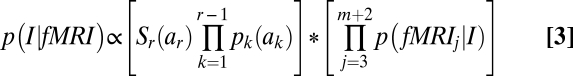The first term in the product is the prior probability and the product in the second term is the conditional probability. The terms p_k(a_k) in the prior probability are the probabilities that the kth interval is of length a _k and S_r(a_r) is the probability of the rth interval surviving at least as long as a_r. These probabilities can be determined from Fig. 2 for On intervals and from the experimental software for Off intervals. The second term contains p(fMRI_j|I), which are the probabilities for the combined fMRI signal on scan j+2 given I’s assignment of scan j to an On or a Off state. The linear classifier determines these from normal distributions fitted to the curves in Fig. 3B.

To calculate the probability that a student is in state r on any scan m one needs to sum the probabilities of all interpretations of length m that end in state r. This can be efficiently calculated by a variation of the forward algorithm associated with hidden Markov models (HMMs) (20). [Because the state durations are variable, the model is technically a hidden semi-Markov process (20). The data and MATLAB code are available at http://act-r.psy.cmu.edu/models under the title of this article.] The predicted state is the highest probability state. The most common HMM algorithm is the Viterbi algorithm, a dynamic programming algorithm that requires knowing the end of the event sequence to constrain interpretations of the events. The algorithm we use is an extension of the forward algorithm associated with HMMs and does not require knowledge of the end of the event sequence. As such, it can be used in real time and is simpler.

Fig. 5 illustrates the performance of this algorithm on a block of problems solved by the first student. Fig. 5A shows the 20 forms of the five equations. Starting in an Off state, going through 20 On states, and ending in an Off state, the student goes through 41 states. Fig. 5B illustrates in maroon the scans on which the algorithm predicts that the student is engaged on a particular equation form. Predictions are incorrect on 19 of the 241 scans, but never off by more than one state. In 18 of these cases, it is one scan late in predicting the state change and in 1 case it is one scan too early.

Although Fig. 5 just illustrates performance for one student and one block, Fig. 6 shows the average performance over the 104 blocks on Day 1 and the 106 blocks on Day 5. The performance is measured in terms of the distance between the actual state and the predicted state in the linear sequence of states in a block. A difference of 0 indicates that the algorithm correctly predicted the state of the scan, negative values are predicting the state too early, and positive values are predicting the state too late. The performance of the algorithm is given in the curve labeled “Both.” On Day 1 it correctly identifies 86.6% of the 22,138 scans and is within one state (usually meaning the same problem) on 94.4% of the scans. Because all parameters are estimated on Day 1, the performance on Day 5 represents true prediction: It correctly identifies 83.4% of the 19,914 scans on Day 5 and is within one state on 92.5% of the scans. To provide some comparisons, Fig. 6 shows how well the algorithm could do given only the simple behavioral model or only the fMRI signal.

Fig. 6.

Performance, measured as the distance between the actual state and the predicted state, using both cognitive model and fMRI, just fMRI, or just a cognitive model on (A) Day 1 and (B) Day 5.

• The fMRI-only algorithm ignores the information relating mouse clicks to duration and sets the probability of all lengths of intervals to be equal. In this case, the algorithm tends to keep assigning scans to the current state until a signal comes in that is more probable from the other state. This algorithm gets 43.9% of the Day 1 scans and 30.6% of the Day 5 scans. It is within one scan on 51.8% of the Day 1 scans and 37.3% of the Day 5 scans. Fig. 5C illustrates typical behavior: it tends to miss pairs of states. This leads to the jagged functions in Fig. 6, with rises for each even offset above 0.

• The model-only algorithm ignored the fMRI data and set the probability of all signals in all states to be equal. Fig. 5D illustrates typical behavior. It starts out relatively in sync but becomes more and more off and erratic over time. It is correct on 21.9% of the Day 1 scans and 50.4% of the Day 2 scans. It is within one scan on 32.9% of the Day 1 scans and 56.9% of the Day 5 scans.

The performances of the fMRI-only and model-only methods are quite dismal. Successful performance requires knowledge of the probabilities of both different interval lengths and different fMRI signals. The relatively high performance on Day 5 is striking, given that it only uses regions and parameters estimated from Day 1.

Discussion

The results illustrate the importance of integrating the bottom-up information from the imaging data with the top-down information from a cognitive model. The current research attempted to hold true to two realities of tutor-based approaches to instruction. First, the model-tracing algorithm must be parameterized on the basis of pilot data and then be applied in a later situation. In the current work, the algorithm were parameterized with an early dataset and tested on a later dataset. Second, the model-tracing algorithm must provide actionable diagnosis in real time; it cannot wait until all of the data are in before delivering its diagnosis. In our case, the algorithm provided diagnosis about the student's mental state in almost real time with a 4-s lag. Knowledge tracing, which uses diagnosis of current student problem solving to choose later problems, does not have to act in real time and can wait until the end of the problem sequence to diagnose student states during the sequence. In this case one could also use the Viterbi algorithm for HMMs (21) that takes advantage of the knowledge of the end of the sequence to achieve higher accuracy. On this dataset, the Viterbi algorithm is able to achieve 94.1% accuracy on Day 1 and 88.5% accuracy on Day 2.

This experiment has shown that it is possible to merge brain imaging with a cognitive model to provide a fairly accurate diagnosis of where a student is in episodes that last as long as 10 min. Moreover, prediction accuracy using both information sources was substantially greater than using either source alone. The performance in Fig. 6 is by no means the highest level of performance that could be achieved. Performance depends on how narrow the distributions of state durations are (Figs. 2 B and D) and the degree of separation between the signals from different states (Fig. 3B). The model leading to the distributions of state durations was deliberately simple, being informed only by number of clicks and a general learning decrease of 0.7 from Day 1 to Day 5. More sophisticated student models, like those in the cognitive tutors, would allow us to track specific students and their difficulties, leading to much tighter distributions of state durations. On the data side, improvement in brain imaging interpretation would lead to greater separation of signals. In addition, other data, like eye movements, could provide additional features for a multivariate pattern analysis.

Materials and Methods

Twelve right-handed members of the Pittsburgh community (seven females, five males), aged 18 to 24 years old, completed the study. Participants provided informed consent according to the Institutional Review Board protocols of Carnegie Mellon University. To create a structure that involved periods of engagement and nonengagement during the scanning sessions, we inserted a 12-s period of one-back between the transformation and evaluation phases and after the evaluation phase. The screen went blank and students saw a sequence of letters presented at the rate of one per 1.25 s. They were to press the mouse if the same letter occurred twice in succession (which happened one-third of the time). This is a minimally engaging task that was intended to keep the student interacting with the interface but prevent them from engaging in algebraic or arithmetic operations. Although each of the sections begins with some instruction, the majority of the students’ time was spent practicing later problems in the section and the imaging data were limited to these practice problems. During these problems, students receive feedback on errors and can receive help if they request it.

Images were acquired using gradient echo-planar image acquisition on a Siemens 3T Allegra Scanner using a standard RF head coil (quadrature birdcage), with 2-s repetition time, 30-ms echo time, 70° flip angle, and 20-cm field of view. We acquired 34 axial slices on each scan using a 3.2-mm thick, 64 × 64 matrix. The anterior commissure-posterior commissure line was on the eleventh slice from the bottom. Acquired images were analyzed using the National Institute of Science system. Functional images were motion-corrected using six-parameter 3D registration (22). All images were then coregistered to a common reference structural MRI by means of a 12-parameter 3D registration (22) and smoothed with a 6-mm full-width half-max 3D Gaussian filter to accommodate individual differences in anatomy.

The 408 regions of interest were created by evenly distributing 4 × 4 × 4-voxel cubes over the 34 slices of the 64 × 64 acquisition matrix. Between-region spacing was 1 voxel in the x- and y-directions in the axial plane, and one slice in the z-direction. The final set of regions was attained by applying a mask of the structural reference brain and excluding regions where less than 70% of the region's original 64 voxels survived.

References

- 1.Koedinger KR, Anderson JR, Hadley WH, Mark M. Intelligent tutoring goes to school in the big city. Int J Artif Intell Educ. 1997;8:30–43. [Google Scholar]
- 2.Ritter S, Anderson JR, Koedinger KR, Corbett A. Cognitive tutor: applied research in mathematics education. Psychon Bull Rev. 2007;14:249–255. doi: 10.3758/bf03194060. [DOI] [PubMed] [Google Scholar]
- 3.Davatzikos C, et al. Classifying spatial patterns of brain activity with machine learning methods: application to lie detection. Neuroimage. 2005;28:663–668. doi: 10.1016/j.neuroimage.2005.08.009. [DOI] [PubMed] [Google Scholar]
- 4.Haxby JV, et al. Distributed and overlapping representations of faces and objects in ventral temporal cortex. Science. 2001;293:2425–2430. doi: 10.1126/science.1063736. [DOI] [PubMed] [Google Scholar]
- 5.Haynes JD, et al. Reading hidden intentions in the human brain. Curr Biol. 2007;17:323–328. doi: 10.1016/j.cub.2006.11.072. [DOI] [PubMed] [Google Scholar]
- 6.Mitchell TM, et al. Predicting human brain activity associated with the meanings of nouns. Science. 2008;320:1191–1195. doi: 10.1126/science.1152876. [DOI] [PubMed] [Google Scholar]
- 7.Abdelnour AF, Huppert T. Real-time imaging of human brain function by near-infrared spectroscopy using an adaptive general linear model. Neuroimage. 2009;46:133–143. doi: 10.1016/j.neuroimage.2009.01.033. [DOI] [PMC free article] [PubMed] [Google Scholar]
- 8.Haynes JD, Rees G. Predicting the stream of consciousness from activity in human visual cortex. Curr Biol. 2005;15:1301–1307. doi: 10.1016/j.cub.2005.06.026. [DOI] [PubMed] [Google Scholar]
- 9.Hutchinson RA, Niculescu RS, Keller TA, Rustandi I, Mitchell TM. Modeling fMRI data generated by overlapping cognitive processes with unknown onsets using Hidden Process Models. Neuroimage. 2009;46:87–104. doi: 10.1016/j.neuroimage.2009.01.025. [DOI] [PubMed] [Google Scholar]
- 10.Anderson JR. How Can the Human Mind Occur in the Physical Universe? New York: Oxford University Press; 2007. [Google Scholar]
- 11.Brunstein A, Betts S, Anderson JR. Practice enables successful learning under minimal guidance. J Educ Psychol. 2009;101:790–802. [Google Scholar]
- 12.Foerster PA. Algebra I. 2nd Ed. Menlo Park, CA: Addison-Wesley Publishing; 1990. [Google Scholar]
- 13.Owen AM, McMillan KM, Laird AR, Bullmore E. N-back working memory paradigm: a meta-analysis of normative functional neuroimaging studies. Hum Brain Mapp. 2005;25:46–59. doi: 10.1002/hbm.20131. [DOI] [PMC free article] [PubMed] [Google Scholar]
- 14.Anderson JR, Betts S, Ferris JL, Fincham JM. Expertise and Skill Acquisition: The Impact of William G. Chase, ed Staszewski J. New York: Taylor Francis; 2010. Can neural imaging be used to investigate learning in an educational task? in press. [Google Scholar]
- 15.Card SK, Moran TP, Newell A. The Psychology of Human-Computer Interaction. Hillsdale, NJ: Erlbaum; 1983. [Google Scholar]
- 16.Green DM, Swets JA. Signal Detection Theory and Psychophysics. New York, NY: Wiley; 1966. [Google Scholar]
- 17.Anderson JR, Qin Y, Sohn M-H, Stenger VA, Carter CS. An information-processing model of the BOLD response in symbol manipulation tasks. Psychon Bull Rev. 2003;10:241–261. doi: 10.3758/bf03196490. [DOI] [PubMed] [Google Scholar]
- 18.Qin Y, et al. The change of the brain activation patterns as children learn algebra equation solving. Proc Natl Acad Sci USA. 2004;101:5686–5691. doi: 10.1073/pnas.0401227101. [DOI] [PMC free article] [PubMed] [Google Scholar]
- 19.Rosenberg-Lee M, Lovett MC, Anderson JR. Neural correlates of arithmetic calculation strategies. Cogn Affect Behav Neurosci. 2009;9:270–285. doi: 10.3758/CABN.9.3.270. [DOI] [PubMed] [Google Scholar]
- 20.Murphy K. Hidden Semi-Markov Models. Boston, MA: Technical Report MIT AI Lab; 2002. [Google Scholar]
- 21.Rabiner RE. A tutorial on Hidden Markov Models and selected applications in speech recognition. Proc Inst Electri Electro Eng. 1989;77:257–286. [Google Scholar]
- 22.Woods RP, Grafton ST, Holmes CJ, Cherry SR, Mazziotta JC. Automated image registration: I. General methods and intrasubject, intramodality validation. J Comput Assist Tomogr. 1998;22:139–152. doi: 10.1097/00004728-199801000-00027. [DOI] [PubMed] [Google Scholar]