Bio-molecule Surfaces Construction via a Higher-Order Level-Set Method

Abstract

We present a general framework for a higher-order spline level-set (HLS) method and apply this to bio-molecule surfaces construction. Starting from a first order energy functional, we obtain a general level set formulation of geometric partial differential equation, and provide an efficient approach to solve this partial differential equation using a C² spline basis. We also present a fast cubic spline interpolation algorithm based on convolution and the Z-transform, which exploits the local relationship of interpolatory cubic spline coefficients with respect to given function data values. One example of our HLS method is demonstrated, which is the construction of bio-molecule surfaces (an implicit solvation interface) with their individual atomic coordinates and solvated radii as prerequisite.

1 Introduction

Given a non-negative function g(x) over a domain Ω ⊂ ℝ³, find a surface Γ in Ω to minimize the energy functional

$$E(\Gamma )={\int }_{\Gamma }g\left(\mathbf{\text{x}}\right)d\mathbf{\text{x}}+\epsilon {\int }_{\Gamma }h\left(\mathbf{\text{x}},\text{n}\right)d\mathbf{\text{x}},$$ (1)

where x and n are surface point and normal to the surface, respectively. Furthermore, h(x,n) is another non-negative function defined over ℝ³ × ℝ³\{0} chosen for regularizing the constructed smooth surface. Constant ε ≥ 0 is to control the regularization effect. Many solid and physical modeling problems, such as surface (solid boundary) reconstruction, and physics-based simulation of deformable interfaces could be formulated as minimizing one kind of energy in the form of (1). By calculating the variation of this energy functional, a partial differential equation (PDE) in the level-set formulation can be generated. In this paper, we propose a higher-order spline level-set method to solve the obtained PDE. To verify the effectiveness of this method, smooth surface constructions experiments are carried out. As illustrative examples, Figure 1 shows the smooth solvent excluded molecular surface construction.

Figure 1.

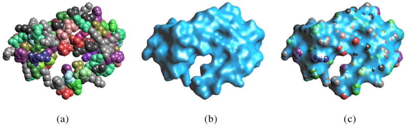
(a) shows the van der Waals surface of a molecule. (b) shows the corresponding solvent excluded molecular surface constructed using our C² tri-cubic spline level-set method. (c) illustrates that the smooth solvent excluded surface constructed encloses the van der Waals surface (a) tightly.

Why Use a Level-Set Method?

In shape deformation simulations, topology changes may occur. This topology change makes parametric form surface tracking difficult even though the hard problem of global parametrization of a discrete surface could be successfully solved. However, implicit form surface (level-set surface) deformation could overcome this difficulty. Thus, level-set method has been a leading subject in many areas (the interested readers are referred to two monographs [1] and [2] for details and references) since the seminal work of Osher and Sethian ([3]) appeared. The level-set method allows one to dynamically deform and track an implicit surface using a governing PDE, which describes various laws of motion depending on geometry, external forces, or a desired energy minimization. Furthermore, the underlining data structure is simple with the computation being restricted to a narrow band surrounding the level-set.

Why Use a Higher-Order Spline Method?

The level-set surfaces obtained from classical level-set methods are generally bumpy due to the use of piecewise tri-linear interpolation from the discrete function data computed on a rectilinear grid. To produce a higher quality surface, a denser grid needs to be used. However, the increased grid resolution substantially increases the computation costs. Another drawback of using discrete data over grids is the non-trivial requirement of estimating derivatives for smooth interpolation. In many surface construction problems, such as the construction of molecular surface, the underlining surface is at least C¹ smooth. Therefore, a smooth level-set function is highly desirable. In this paper, second-order geometric partial differential equations are required to be solved with mean curvature involved. Therefore, we use C² tri-cubic spline as the level-set function basis. Note that tri-cubic is the lowest order of B-spline that could achieve C² in 3D. The advantages using C² spline function basis include:

1. Since the level-set function is C², the level-set surface is G². There does exist a finite number of critical level-set values where the level-set surface may have a finite number of isolated singular points (i.e., the gradient of the level-set function vanishes). However working in a finite precision numerical domain one can automatically avoid this finite set of critical level-set values.

2. Derivatives up to the second order and curvatures, which appear in the governing geometric partial differential equations, can be easily and accurately computed from the C² level-set function.

Main Contributions

We derive and describe an efficient approach of higher-order local level-set method to solve PDEs. Using a first order energy functional, a second order geometric PDE in the level-set formulation is obtained. To achieve higher efficiency in using tri-cubic spline functions for solving PDEs, a fast and exact cubic spline interpolation algorithm is presented. Furthermore, the local property of cubic spline function is analyzed. Based on this analysis, a local spline level-set method is implemented. Though we use tri-cubic spline functions here, we could easily use splines of any other orders as well. We apply our method to the smooth construction of bio-molecular solvation interfaces. Our construction method is simple, efficient and error bounded.

The rest of the paper is organized as follows. Section 2 outlines the main algorithm steps for solving the geometric PDE. The details of these steps are considered in the sections that follow. In Section 3, we describe a fast spline interpolation algorithm. The derivation of the interpolation algorithm is given in our technical report [4]. The initialization, evolution and re-initialization steps in the main algorithm are discussed in Section 4. Application to bio-molecular surfaces construction is considered in Sections 5. Section 6 concludes the paper.

2 Algorithm Outline

By calculating the variation of energy functional (1), we obtain the following evolution equation (see [5])

$$\begin{array}{l}\frac{\partial \phi }{\partial t}=\left(g+\epsilon h\right)\text{div}\left(\frac{\nabla \phi }{\Vert \nabla \phi \Vert }\right)\Vert \nabla \phi \Vert \hfill \\ +\epsilon \text{div}\left(\text{P}{\nabla }_{n}h\right)\Vert \nabla \phi \Vert +2{\left[\nabla \left(g+\epsilon h\right)\right]}^T\nabla \phi \hfill \\ =L\left(\phi \right)+H\left(\nabla \phi \right),\hfill \end{array}$$ (2)

where

$$\begin{array}{l}L\left(\phi \right)=\left(g+\epsilon h\right)\text{div}\left(\frac{\nabla \phi }{\Vert \nabla \phi \Vert }\right)\Vert \nabla \phi \Vert ,\hfill \\ H\left(\nabla \phi \right)=\epsilon \mathit{\text{div}}\left(\text{P}{\nabla }_{n}h\right)\Vert \nabla \phi \Vert +2{\left[\nabla \left(g+\epsilon h\right)\right]}^T\nabla \phi ,\hfill \end{array}$$

$\text{P}=\text{I}-\frac{\nabla \phi }{\Vert \nabla \phi \Vert }\otimes \frac{\nabla \phi }{\Vert \nabla \phi \Vert }$ is a projection operator onto the tangent space and I indicates the identity mapping. ∇ and ∇_n denote the usual gradient operator with respect to x and n, respectively. Note that L(φ) is a parabolic term and H(∇φ) is a hyperbolic term. Hence, in solving equation (2) in the following, the first order term H(∇φ) is computed using an upwind scheme (see [6] for the reason) over a finer grid, and the higher order term L(φ) is computed using a spline presentation defined on a coarser grid. In the experiments carried out in this paper, we always choose h(x,n) to be 1 for simplicity.

Consider the solution of equation (2) over the domain Ω = [a,b] × [c,d] × [e,f] ⊂ ℝ³. For simplicity, we assume b − a = d − c = f − e > 0 and the domain Ω is uniformly partitioned with vertices $G_0={\{{\mathbf{\text{x}}}_{\mathit{\text{ijk}}}\}}_{\mathit{\text{ijk}}=0}^n:={\{x_i\}}_{i=0}^n\times {\{y_j\}}_{j=0}^n\times {\{z_k\}}_{k=0}^n$, where

$$x_i=a+i\Delta x,y_j=c+j\Delta y,z_k=e+k\Delta z,$$

and Δx = Δy = Δz = (b − a)/n. Let G_l be the set of grid points generated by bisecting G₀ l times. Let φ be a piecewise tri-linear level-set function over the grid G_l, Φ be a tri-cubic spline approximation of φ over the grid G₀. In general, l is chosen to be 0 or 1 or 2. In our implementation, we take l=1. If l = 0, Φ and φ are defined on the same grid G₀, which is the simplest case. The aim of the following algorithm is to compute the spline level set function Φ.

Algorithm Steps

1. Initialization. Given an initial Γ, construct a piecewise tri-linear level-set function φ over the grid G_l. If necessary, apply a reinitialization step to set φ to be a signed distance function to Γ (see section 4.2 for details). Convert φ to Φ (see Section 3).

2. Evolution. Resample Φ to obtain a new φ over the grid G_l. Compute L(Φ) and H(∇φ) in the thin shell (traditionally called a narrow band for curve evolution) N = {(x_i,y_j, Z_k) ∈ G_l : |φ(x_i,y_j,z_k)| < ℋ}. Update φ in N for one time step to get φ̃ by an ODE time stepping method (see section 4.3).

3. Re-initialization. Apply re-initialization step to φ̃ in the shell

   $$\begin{array}{l}N=\{(x_i,y_j,z_k)\in G_l:\\ \underset{-1\le \mu ,\nu ,\lambda \le 1}{\text{min}}|{\phi }_{i+\mu ,j+\nu ,k+\lambda }|\le \mathscr{H}\}\end{array}$$

   to get a new φ (see section 4.4). Convert φ to Φ (see Section 3). Go back to step 2 if the termination condition is not satisfied.

4. Iso-contouring. Extract 3-sided or 4-sided iso-surface patches (vertices with normals) of Φ = c, where c is a given iso-value. G¹ approximate these patches by parametric surfaces.

Remark 2.1

For the problem of molecular surface construction, the grid size G₀ should be less than the radii of atoms so that atoms are distinguishable from the level set surface. In our implementation, the grid size is chosen to be one-half of the minimal value of the atom radii.

Remark 2.2

The aim of using l > 0 is to make φ a more accurate approximation of the signed distance function. The larger the value of l we use, the better approximation of the signed distance function we have. Since the scanned data to be approximated in general suffers from noise, we use the approximation Φ over a coarse grid G₀ for denoising.

3 Fast Cubic Spline Interpolation

3.1 Algorithm

Let

$${\beta }^3\left(x\right)=\{\begin{array}{cc}\frac{2}{3}-x^2+\frac{1}{2}{\left|x\right|}^3,\hfill & 0\le \left|x\right|<1,\hfill \\ \frac{1}{6}{\left(2-\left|x\right|\right)}^3,\hfill & 1\le \left|x\right|<2,\hfill \\ 0,\hfill & 2\le \left|x\right|.\hfill \end{array}$$

be the cubic B-spline base function over the knots {−2,−1,0,1,2}, and let

$$s\left(x\right)=\sum _{i=1}^{n-1}{c}_i{\beta }^3\left(x-i\right)$$ (3)

be a cubic spline function. Then the spline interpolation problem is to determine the coefficients $\text{c}={\{c_i\}}_{i=1}^{n-1}$ such that the following interpolation conditions

$$s\left(k\right)=\sum _{i=1}^{n-1}{c}_i{\beta }^3\left(k-i\right),k=1,\dots ,n-1$$ (4)

are satisfied for any given function values ${\left\{s\left(k\right)\right\}}_{k=1}^{n-1}$. Such a problem could be easily solved by solving the linear system (4) directly for the unknowns c₁, …,c_n−1. The algorithm derived here is in O(n) complexity. Given two function values s(0) and s(n), system (4) could be augmented as

$$s\left(k\right)=\sum _{i=1}^{n-1}{c}_i{\beta }^3\left(k-i\right),k=0,\dots ,n.$$

Recursive Algorithm

Using the initial values

$$c_0^{+}=-\frac{1}{1-z_1^{2n}}\sum _{k=1}^{n-1}s\left(k\right)z_1^k(1-z_1^{2\left(n-k\right)}),c_n^{-}=0,$$ (5)

the recursive process

$$\begin{array}{l}{c}_k^{+}=s\left(k\right)+z_1{c}_{k-1}^{+},k=1,2,\dots ,n-1,\\ c_k^{-}=z_1(c_{k+1}^{-}-c_k^{+}),k=n-1,n-2,\dots ,1,\end{array}$$

yields exact B-spline coefficients $c_i=6c_i^{-}$ of the interpolation problem, where ${\mathit{\text{z}}}_1=\sqrt{3}-2$.

Remark 3.1

The computation of ${\mathit{\text{c}}}_0^{+}$ can be accelerated by neglecting small terms. Given an error control tolerance ε, we compute

$$K=\left[\frac{\text{log}\left(\epsilon \right)}{\text{log}(|z_1|)}\right].$$

If n > K, we replace ${\mathit{\text{c}}}_0^{+}$ in (5) with

$$c_0^{+}=-\frac{1}{1-z_1^{2n}}\sum _{k=1}^{n-1}s\left(k\right)z_1^k,$$

which can be computed by the Horner scheme for evaluating a polynomial.

3.2 Locality of Spline Interpolation

Since the basis function β³ (x) is locally supported, the kth coefficient c_k of the spline function (3) merely has influence on s(x) within the interval (k − 2, k + 2). A set of function values {s(i)}

$$s\left(i\right)=\{\begin{array}{cc}0,& i\ne k,\\ 1,& i=k,\end{array}$$

define a set of coefficients {c_i} with none of them zero. However, the coefficients c_k±l are decreasing with respect to l. To see this, let us compute $c_k^{-}$. Suppose that the interpolation problem considered is over (−∞,+∞). From the definition of $c_k^{-}$, we have

$$c_k^{-}=-z_1(1+z_1^2+z_1^4+\cdots )=-\frac{z_1}{1-z_1^2}=\frac{\sqrt{3}}{6}.$$

Similarly,

$$c_{k\pm l}^{-}=-z_1^{l+1}(1+z_1^2+z_1^4+\cdots )=z_1^l\frac{\sqrt{3}}{6},$$

for l = 0,1,2, …. Therefore,

$$c_{k\pm l}=z_1^l\sqrt{3},l=0,1,2,\mathrm{....}$$

Note that ${\mathit{\text{z}}}_1=\sqrt{3}-2\approx -0.2679491924$ and c_k±l will decrease to zero rapidly. The first ten terms are 1.732, −0.464, 0.124, −0.0333, 0.00893, −0.00239, 0.000641, −0.000172, 0.0000460, −0.0000123. Given a threshold ε, the coefficients c_k±l with |c_k±l| < ε could be ignored. We take ε = 0.005. Therefore, we keep the terms

$$c_{k\pm l},l=0,1,2,3,4.$$

If we require that the second order derivatives have accuracy ε, we need to determine l, such that

$${|z_1|}^l\sqrt{3}<\Delta x^2\epsilon ,$$ (6)

where Δx is the spacing of the knots.

Remark 3.2

Higher dimensional spline interpolation can be recursively computed by using lower dimensional spline computations. We do not exposit this here.

3.3 Conversion of Piecewise Tri-linear Functions to Tri-cubic Splines

Let φ_l be a piecewise tri-linear function over the grid G_l. Now we intend to convert it approximately to a trivariate tri-cubic spline function Φ over the grid G₀. If l = 0, the conversion algorithm is described in section 3.1. Now we assume l > 0. The conversion could be done in several ways. One simple way is to use Φ to interpolate φ_l over the grid G_l in the least square sense. This requires us to solve a linear system with size n³, which is the number of grid in G₀. Another algorithm is to convert φ_l to a spline function Φ_l over the grid G_l firstly, and then use the knots removal algorithm of spline function to obtain Φ_l−1, Φ_l−2, …, Φ₀ repeatedly. Since Φ_k may not be represented exactly by Φ_k−1, a least square approximation has to be used. This also leads to solving a linear system.

The method we use in this paper is to convert φ_l to φ_l−1, φ_l−2, …, φ₀, where φ_k is a piecewise tri-linear function over the grid G_k. Finally, we convert φ₀ to Φ using the conversion algorithm described in section 3.1. For converting φ_k to φ_k−1, we use a local tri-linear function at each grid point of G_k−1 to interpolate φ_k at 27 neighbor grid points of G_k in the least square sense. This leads to an 8×8 linear system of equations for each of the grid point of G_k−1. Note that all these systems have the same coefficient matrix. Hence, we only need to inverse the matrix once. Furthermore, this conversion are conducted only in a neighborhood of the level-set surface (see Section 4). Therefore it is very efficient.

4 Solving the PDE by a Local Level-set Method

In this section, we describe a local level-set method, using a tri-cubic spline level-set function Φ over the grid G₀ and a piecewise tri-linear level-set function φ over the grid G_l, which represents a signed distance function. We first define a thin shell around the interface in which the level-set function is updated. Then we determine the initial level-set function followed by the evolution of the level-set function. Finally we explain the reinitialization step.

4.1 Thin Shell of a Tri-cubic Spline

During the evolution process, we confine the movement of the level-set surface to no more than one grid size Δx of G_l for each time step. Since ‖∇φ‖ = 1 before the movement, we require that function values, and up to the second order partial derivatives of φ, are accurately computed (within the given error tolerance) in the c + Δx neighborhood of the interface, where c is the iso-value used for extracting the level-set (see the last step of main algorithm in Section 2). From (6), we define the thin shell as

$$N=\left\{\mathbf{\text{x}}\in G_l:\left|\phi \left(\mathbf{\text{x}}\right)\right|\le \mathscr{H}\right\},$$

where

$$\mathscr{H}=\left[\frac{\text{log}{\left(\Delta x\right)}^2\epsilon -\text{log}\sqrt{3}}{\text{log}|z_1|}+2\right]\Delta x+|c|.$$ (7)

As mentioned before, we take ε = 0.005. Function values that are beyond ℋ are truncated by ℋ, meaning if φ (x) > ℋ, then set φ (x) as ℋ, if φ(x) < −ℋ, then set φ(x) as −ℋ. The evolution of φ is performed in this thin shell. The time step is so determined that the function values of φ are changed not more than Δx. By using an explicit Euler method, this is easy to achieve. After the evolution step, the function φ is truncated by ℋ.

In the re-initialization step, the thin shell is updated by introducing new grid points that are the neighbor points of the previous thin shell, and furthermore by removing the points whose values are greater than ℋ in magnitude.

4.2 Initialization

Let Γ⁰ be a given initial closed surface with interior ⊂ ℝ³. We define an initial level-set function φ⁰(x) in ℝ³ satisfying

$$\{\begin{array}{cc}{\phi }^0\left(\mathbf{\text{x}}\right)<0\hfill & \text{in}\mathcal{D},\hfill \\ {\phi }^0\left(\mathbf{\text{x}}\right)=0\hfill & \text{on}{\Gamma }^0,\hfill \\ {\phi }^0\left(\mathbf{\text{x}}\right)>0\hfill & \text{elsewhere}.\hfill \end{array}$$ (8)

Γ⁰ may be given as a close triangular surface mesh, or a level-set of a given function. For each of these two cases, the initial φ⁰ needs to be computed differently.

(a) Γ⁰ is a surface mesh

If Γ⁰ is a surface mesh, we first compute the Euclidean distance from the grid points to the surface mesh using a local fast method (see Algorithm 4.1), and then we specify negative/positive signs to the distance values for the grids inside/outside the surface (see Algorithm 4.2). Since the function values need to be exact only in the thin shell, we compute distance values for the grid points locally around each triangle within the distance ℋ. This is done by the following algorithms.

Algorithm 4.1. Distance Computation

1. Set initial value for each grid point to be ℋ.

2. For each triangle of the mesh, find a containing cube such that the distance of the cube boundary to the triangle is no less than ℋ. For each grid point in the cube, compute the distance from the grid point to the triangle. If this distance is less than the existing value previously computed, then replace it with the newly computed one.

Algorithm 4.2. Sign Designation

1. Perturb the vertices of the given triangular surface mesh to meet the following two requirements. (i) The x-components of all the face normals are not zero; (ii) The projections of all the edges of the mesh onto the yz-plane do not pass through any grid point on this plane.

2. Compute distance from the grid points to the (perturbed) surface mesh using Algorithm 4.1.

3. First we associate each grid point $\mathbf{\text{q}}\in {\left\{{\mathbf{\text{q}}}_{jk}\right\}}_{jk=0}^n:={\left\{y_j\right\}}_{j=0}^n\times {\left\{z_k\right\}}_{k=0}^n$ on the yz-plane with a set of numbers, called q-pool. This pool is empty at beginning. Let Δ_x be the projection of the triangle Δ of the surface mesh onto the yz-plane. For each grid point q ∈ Δ_x, compute the intersection of the line segment [x,q]^T ∈ ℝ³, x ∈ [a,b] with the triangle Δ. Put the x-component of the intersection point into q-pool.

4. After the computation above, we have a pool for each grid point in the yz-plane. Then we sort the numbers in each of the pool in the increasing order. Let t₁ < t₂ < … < t_k be the sequence in the q-pool. Then if a + jΔx is in the interval [t_i,t_i+1], the sign to the grid point [a+jΔx, q]^T is set to be (−1)ⁱ, where t₀ = a, t_k+1 = b.

Remark 4.1

The aim of the perturbation in the first step of Algorithm 4.2 is to make the intersection of the line segment [x,q]^T, x ∈ [a,b] with Δ to be unique and there is no duplicated numbers in each of q-pool. This perturbation is not harmful to the surface construction algorithm, since Γ⁰ is served as an initial surface.

Remark 4.2

The time complexities of both Algorithm 4.1 and 4.2 are linear with respect to the number of triangles of the given mesh.

(b) Γ⁰ is a level-set

If Γ⁰ is a level-set {x : d(x) = c} of a smooth function d(x), a naive method is to first extract the level-set surface and then compute a signed distance function using the method described earlier. Since extracting iso-surface is not a trivial task, we seek a more efficient method. Suppose that ∇d(x) ≠ 0, x ∈ Γ⁰. Then a simple way is to use d(x) − c or c − d(x) as the initial φ⁰. For example, in the problem of solvent excluded surface construction, d(x) is a Gaussian map, c=1 (see Section 5).

4.3 Evolution

Suppose that we have an initial φ⁰ satisfying (8). First we apply the local re-initialization step, if necessary, to set φ⁰ to be the signed distance function of Γ⁰ (see section 4.4). Then we define a thin shell around Γ⁰ by

$$N^0=\{\mathbf{\text{x}}\in G_l:|{\phi }^0\left(\mathbf{\text{x}}\right)|<\mathscr{H}\}.$$

To prevent numerical oscillations at the boundary of the thin shell, we introduce a cubic cut-off function c(x) in (9), which is defined by C¹ Hermite interpolating the boundary data on [ℋ₀,ℋ]

$$c\left(x\right)=\{\begin{array}{cc}1\hfill & \text{if}\left|x\right|\le {\mathscr{H}}_{0,}\hfill \\ \frac{{\left(\left|x\right|-\mathscr{H}\right)}^2\left(2\left|x\right|+\mathscr{H}-3{\mathscr{H}}_0\right)}{{\left(\mathscr{H}-{\mathscr{H}}_0\right)}^3}\hfill & \text{if}{\mathscr{H}}_0<\left|x\right|\le \hfill \\ 0\hfill & \text{if}\left|x\right|>\mathscr{H},\end{array}\mathscr{H},$$

where ℋ₀ is chosen to be 0.5ℋ. Our experiments show that linear cut-off function works equally well. We update φ⁰ by solving the following equation,

$$\{\begin{array}{c}\frac{\partial \phi }{\partial t}=c\left(\phi \right)\left[L\left(\phi \right)+\mathscr{H}\left(\nabla \phi \right)\right],\hfill \\ \phi \left(\mathbf{\text{x}},0\right)={\phi }^0\left(\mathbf{\text{x}}\right),\hfill \end{array}$$ (9)

on N⁰ for one time step and get φ¹(x). The time step is chosen such that the interface moves less than one grid size Δx. At each grid point x_ijk in the thin shell N⁰, compute ν⁰(x_ijk) = c(φ⁰(x_ijk))[L(Φ⁰(x_ijk)) + H(∇φ⁰(x_ijk))]. Let

$$\tau =\text{min}\left\{\Delta x,\Delta x/\underset{{\mathbf{\text{x}}}_{\mathit{\text{ijk}}}\in N^0}{\text{max}}\left|{\nu }^0\left({\mathbf{\text{x}}}_{\mathit{\text{ijk}}}\right)\right|\right\}.$$

Then update φ⁰ by the explicit Euler scheme

$${\phi }^1({\mathbf{\text{x}}}_{\mathit{\text{ijk}}})={\phi }^0({\mathbf{\text{x}}}_{\mathit{\text{ijk}}})+\tau {\nu }^0({\mathbf{\text{x}}}_{\mathit{\text{ijk}}}),{\mathbf{\text{x}}}_{\mathit{\text{ijk}}}\in N^0.$$

Since φ¹ is no longer a signed distance function, a re-initialization step is required (see section 4.4) to get a new φ¹ and a new thin shell N¹. The process from φ⁰ to φ¹ described above is repeated to get a sequence {φ^m}_m≥0 of φ, and a sequence of thin shells {N^m}_m≥0, until the following termination conditions

$$\underset{{\mathbf{\text{x}}}_{\mathit{\text{ijk}}}\in N^m}{\text{max}}|{\nu }^m({\mathbf{\text{x}}}_{\mathit{\text{ijk}}})|<\epsilon \text{and}m<\text{M}$$ (10)

are satisfied. We choose ε = 0.001. M is a given upper bound of the iteration number. We choose M = n, where n³ is the number of grid points in G_l.

Remark 4.3

The solution to equation (2) may have discontinuous derivatives, even if the initial data is smooth (see [6]). Using simple central difference to approximate the first order term is not appropriate. Hence, we use monotone and upwind scheme for Hamilton-Jacobi equations as developed in [6] for computing H(∇φ^m). The higher order term L(φ^m) is computed from the spline function Φ^m directly. Four monotone discretization schemes (Lax-Friedrichs scheme, Godunov type scheme, Local Lax-Friedrichs scheme and Roe with LLF entropy correction) have been reviewed in [6]. We use Godunov's scheme because it is also upwinding.

4.4 Adaptive Re-initialization

To simplify the notation, let φ^m(x) be denoted by φ (x). In general, it is impossible to prevent φ (x) from deviating away from a signed distance function. Flat and/or steep regions will develop around the interface, making further computation and contour plotting highly inaccurate. Hence a re-initialization step to reset the level-set function φ (x) to be a signed distance function to the interface {x : φ (x) = 0} is necessary.

Re-initialization here is a process of replacing φ (x) by another function φ̃ (x) that is the signed distance function to the zero level-set of φ and then taking this new function φ̃ (x) as the initial data to use until the next round of re-initialization. To achieve this goal, people usually solve the following equation (see [7]) for the unknown function d (x,τ)

$$\{\begin{array}{c}\frac{\partial d}{\partial \tau }+S\left(d\right)\left(\Vert \nabla d\Vert -1\right)=0,\hfill \\ d\left(\mathbf{\text{x}},0\right)=\phi \left(\mathbf{\text{x}}\right),\hfill \end{array}$$ (11)

where S(d) is a sign function. We propose to solve the following Hamilton-Jacobi equation,

$$\{\begin{array}{c}\frac{\partial d}{\partial \tau }+S\left(d\right)(\nabla d^T\nabla d-1)=0,\hfill \\ d\left(\mathbf{\text{x}},0\right)=\phi \left(\mathbf{\text{x}}\right).\hfill \end{array}$$ (12)

for its steady state solution, with S(d) approximated by

$$s=\frac{d}{\sqrt{d^2+{\left|Dd\right|}^2\Delta x^2}},$$ (13)

where Dd is a discrete approximation of ∇d. The advantages of using (12) instead of (11) is that the right hand side of (12) is a smooth function of d, and it also facilitates the usage of semi-implicit temporal discretization scheme.

Discretization

Again, we use the Godunov scheme (see [6]) for the spatial discretization because it is monotone and upwinding. The scheme is described abstractly in [6] for a 2D problem. Here we present the details for our 3D problem (12)

$$\begin{array}{l}{d}_{\mathit{\text{ijk}}}^{n+1}=d_{\mathit{\text{ijk}}}^n-\Delta \tau s_{\mathit{\text{ijk}}}^{+}(\text{max}[{\left(a^{+}\right)}^2,{\left(b^{-}\right)}^2]\hfill \\ +\text{max}[{\left(c^{+}\right)}^2,{\left(d^{-}\right)}^2]+\text{max}[{\left(e^{+}\right)}^2,{\left(f^{-}\right)}^2]-1)\hfill \\ -\Delta \tau s_{\mathit{\text{ijk}}}^{-}(\text{max}[{\left(a^{-}\right)}^2,{\left(b^{+}\right)}^2]+\text{max}[{\left(c^{-}\right)}^2,{\left(d^{+}\right)}^2]\hfill \\ +\text{max}[{\left(e^{-}\right)}^2,{\left(f^{+}\right)}^2]-1),\hfill \end{array}$$ (14)

where S_ijk is the approximation to S(d_ijk) with (13), (x)⁺ = max(x,0), (x)⁻ = min(x,0); a, …, f are defined by

$$\begin{array}{ccc}a=D_x^{-}{d}_{\mathit{\text{ijk}}}^n,& c=D_y^{-}{d}_{\mathit{\text{ijk}}}^n,& e=D_z^{-}{d}_{\mathit{\text{ijk}}}^n,\\ b=D_x^{+}{d}_{\mathit{\text{ijk}}}^n,& d=D_y^{+}{d}_{\mathit{\text{ijk}}}^n,& f=D_z^{+}{d}_{\mathit{\text{ijk}}}^n,\end{array}$$

respectively, where $D_x^{\pm }{d}_{\mathit{\text{ijk}}},D_y^{\pm }{d}_{\mathit{\text{ijk}}}$ and $D_z^{\pm }{d}_{\mathit{\text{ijk}}}$ denote the one-sided divided differences at the grid point x_ijk in the x, y and z directions, separately. These one-sided differences are computed by ENO (essentially non-oscillatory) interpolation (see [6]). Scheme (14) is easily seen to be monotone; i.e., the right hand side of (14) is a nondecreasing function of all the $d_{\mathit{\text{ijk}}}^n$ if

$$\frac{\Delta \tau }{\Delta x}|s_{\mathit{\text{ijk}}}|\le \frac{1}{3}.$$

With the same time step restriction, this scheme is also upwind.

Adaptive Updating the Thin Shell

During the process of re-initialization, function values around the level-set change, and so the thin shell defined by {x ∈ G_l : |φ(x)| < ℋ} should be updated correspondingly. This is automatically achieved by including new grid points with at least one of their one-ring neighbor grid points with value less than ℋ. Additionally we throw away the old grid points in the current thin shell where the function values and function values of all their one-ring neighbor grid points are all greater than ℋ.

5 Smooth Bio-molecular Surfaces Construction

In this section, we use our higher order level-set method with C² tri-cubic spline functions to construct bio-molecular interfaces. As is well known, there are typically three types of molecular surfaces (e.g. [8]): the van der Waals surface (VWS), the solvent-accessible surface (SAS), and the solvent-excluded surface (SES) or Connolly surface ([9]). The van der Waals surface is defined from the van der Waals radii of the atoms, which is the boundary of the region formed by the union of all the spheres (atoms). The SAS introduced by Lee-Richards is defined to be the locus of the center of the rolling sphere (always water molecule) which makes contact with the VWS surface ([10]). Hence the SAS is an inflated VWS with a probe radius of 1.4 Angstroms. The solvent-excluded surface is the solvent (sphere) surface inside of which the probe sphere never intrudes. In other words, SES is the offset surface of SAS in the inward direction with the solvent probe radius as the offset radius. This kind of surface can be represented by Alpha shapes ([11, 12, 13]). The Alpha shape technique has been extensively used for molecular surface modeling (e.g. [14]), area and volume computation and cavity and pocket recognition (e.g. [11, 15]). This technique requires a complex geometric data structure.

Gaussian blurred maps ${\sum }_{i=1}^m{e}^{-d({\Vert \mathbf{\text{x}}-{\mathbf{\text{x}}}_i\Vert }^2-r_i^2)/r^2}$ have been frequently used in the molecular surface construction (see [16, 17, 18, 19]). Both VWS and SAS can be easily approximated by the level-set of the Gaussian map within any given tolerance by properly choosing the parameter d. However, the Gaussian map method cannot generate an accurate approximation to the SES (see Figure 5(a)). It is well known that SES is an important molecular surface (dielectric interface) for many applications, such as electrostatic energy computation (see [20]), various simulations (see [21]). Hence, we focus our attention in this section on the computation of SES using our HLS method.

Structural model of molecule M consisting of a collection of atoms with centers ${\{{\mathbf{\text{x}}}_i\}}_{i=1}^m$ and radii ${\{r_i\}}_{i=1}^m$ (see Figure 3(a)) is retrievable from the Protein Data Bank (PDB). To construct the SES for M, we minimize the energy functional

Figure 3.

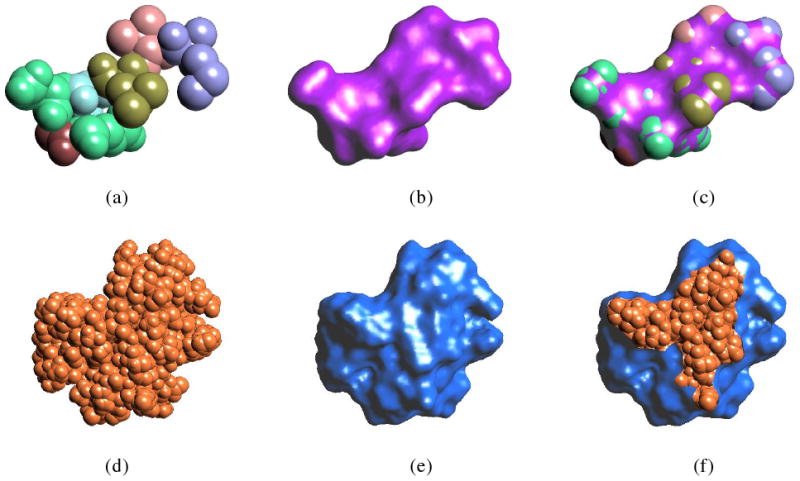
(a) and (d) show the van der Waals surface (VWS). (b) and (e) are the corresponding solvent excluded surface (SES) constructed. (c) and (f) illustrate the tight enclosure of the smooth SES to the VWS.

$$E(\Gamma )={\int }_{\Gamma }g{\left(\mathbf{\text{x}}\right)}^{2}d\mathbf{\text{x}}+\epsilon {\int }_{\Gamma }d\mathbf{\text{x}},$$ (15)

where

$$g\left(\mathbf{\text{x}}\right)=1-\sum _{i=1}^m{e}^{-C({\Vert \mathbf{\text{x}}-{\mathbf{\text{x}}}_i\Vert }^2-{\stackrel{\sim }{r}}_i^2)},{\stackrel{\sim }{r}}_i=r_i+r_b,$$

with r_b the probe radius, which is usually 1.4 Å. The constant C > 0 is so determined that g(x) = 0 is an approximation of the solvent accessible surface within a given tolerance (see Figure 3(b) and section 5.1). The second term of (15) is used to regularize the constructed surface, where ε is a small number. In the examples provided in the following, we choose ε as 0.1. The corresponding level-set formulation of the evolution equation for the energy (15) is

$$\begin{array}{l}\frac{\partial \phi }{\partial t}=(g^2+\epsilon )\text{div}\left(\frac{\nabla \phi }{\Vert \nabla \phi \Vert }\right)\Vert \nabla \phi \Vert +4g{\left(\nabla g\right)}^T\nabla \phi \hfill \\ =L\left(\phi \right)+H\left(\nabla \phi \right),\hfill \end{array}$$ (16)

where

$$\begin{array}{l}L\left(\phi \right)=(g^2+\epsilon )\text{div}\left(\frac{\nabla \phi }{\Vert \nabla \phi \Vert }\right)\Vert \nabla \phi \Vert ,\hfill \\ H\left(\nabla \phi \right)=4g{\left(\nabla g\right)}^T\nabla \phi .\hfill \end{array}$$

As before, the first order term H(∇φ) is computed using an upwind scheme over a finer grid, the higher order term L(φ) is computed using a spline presentation defined on a coarser grid. If φ is a signed distance function and a steady solution of equation of (16), then the iso-surface φ = − r_b is an approximation of SES (see Figure 3(c)). The algorithm in Section 2 could be specialized as follows.

Algorithm 5.1. Solvent Excluded Surface Construction

1. Compute g(x) over the grid G_l (see section 5.2 for the fast computation of g(x)).

2. Compute an initial φ by taking φ(x) = g(x) and then update it with a re-initialization step, such that ‖∇φ‖ = 1 (see section 4.4).

3. Update φ by solving equation (16) for one time step using a divided difference method (see Section 4).

4. Re-initialize φ, and then go back to the previous step if the stopping criterion (10) is not satisfied.

5. Generate iso-surface {x : Φ(x) = −r_b}, which is the required approximation of SES.

Remark 5.1

In step 2, φ(x) may change rapidly, we may slow down the changes of φ by dividing it with a constant before taking the re-initialization step. Since the gradient of $e^{-C[{\Vert \mathbf{\text{x}}-{\mathbf{\text{x}}}_i\Vert }^2-{\stackrel{\sim }{r}}_i^2]}$ is $-2C{e}^{-C[{\Vert \mathbf{\text{x}}-{\mathbf{\text{x}}}_i\Vert }^2-{\stackrel{\sim }{r}}_i^2]}{[x-x_i,y-y_i,z-z_i]}^T$, the length of the gradient is approximately $2C{\stackrel{\sim }{r}}_i$ at the sphere surface $\{\mathbf{\text{x}}:\Vert \mathbf{\text{x}}-{\mathbf{\text{x}}}_i\Vert ={\stackrel{\sim }{r}}_i\}$. Hence we normalize the function φ by dividing it with $2C\ast {\text{max}}_i{\stackrel{\sim }{r}}_i$.

5.1 Error Bounded Approximation

Let ε be a given error tolerance for the constructed SES. We determine the constant C to satisfy this error constraint. Assume that at each surface point of SAS, at most k atomic spheres intersect. Each of these spheres thus has a maximum contribution of 1/k to the Gauss map g(x) at such surface points of the SAS. That is

$$e^{-C[{\Vert \mathbf{\text{x}}-{\mathbf{\text{x}}}_i\Vert }^2-{\stackrel{\sim }{r}}_i^2]}=e^{-C[{({\stackrel{\sim }{r}}_i+\epsilon )}^2-{\stackrel{\sim }{r}}_i^2]}=\frac{1}{k}.$$

From this we cobtain

$$C\approx \frac{\text{ln}k}{2{\stackrel{\sim }{r}}_i\epsilon }.$$

For instance, if k is 4, we choose ε = 0.01, and C is thus chosen to be $\frac{50\text{ln}4}{r_b+{\text{min}}_i{r}_i}$.

5.2 Fast Computation of Gaussian Map

Since each term $e^{-C[{\Vert \mathbf{\text{x}}-{\mathbf{\text{x}}}_i\Vert }^2-{\stackrel{\sim }{r}}_i^2]}$ in g(x) decreases rapidly as ‖x − x_i‖ increases, we evaluate $e^{-C[{\Vert \mathbf{\text{x}}-{\mathbf{\text{x}}}_i\Vert }^2-{\stackrel{\sim }{r}}_i^2]}$ locally around x_i. Suppose that we evaluate it for x such that

$$e^{-C[{\Vert \mathbf{\text{x}}-{\mathbf{\text{x}}}_i\Vert }^2-{\stackrel{\sim }{r}}_i^2]}>\epsilon ,$$

where ε is a given threshold value (e.g., we take ε = 10⁻⁵). We have

$${\Vert \mathbf{\text{x}}-{\mathbf{\text{x}}}_i\Vert }^2<{\stackrel{\sim }{r}}_i^2-\frac{\text{ln}\epsilon }{C}.$$ (17)

Hence, we only evaluate the term over the grids within the spherical range defined by (17). For the simplicity of implementation, we determine a minimal bounding cube containing the sphere defined by (17), and evaluate the function within the cube. The time complexity of this algorithm is obviously linear with respect to the number of atoms.

5.3 Illustrative Examples

We have implemented our higher-order level-set algorithm in the molecular visualization software package TexMol ([22]). We present a few examples to demonstrate the quality of the SES for molecules from the PDB. In these examples, the solvent probe (water molecule) radius is chosen to be 1.4. Figure 4 shows two molecular surface constructions, where figures (a) and (d) show the VWS, respectively, (b) and (e) are the corresponding SES. (c) and (f) illustrate how the smooth SES encloses the VWS tightly and how the SES transits between the atoms (spheres) smoothly.

Figure 4.

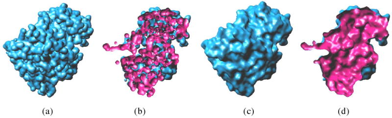
Comparing the results of Gaussian blurring and our new method. (a) and (b) show the result of Gaussian blurring with d = −2.3. (c) and (d) are the level-set surfaces of φ = −1.4 of the level set method. (b) and (d) show cross-section views of (a) and (c), respectively, by a cross-section plane perpendicular to the view direction. The inner side of the surface is rendered in pink to differentiate with the outer side.

Figure 5 shows the difference between our method with Gaussian blurring method (e.g. [19]) for an enzyme with 1UDI as its PDB ID. The surface of Gaussian blurring is defined by {x ∈ ℝ³ : g(x) = 1}, where

$$g\left(\mathbf{\text{x}}\right)=\sum _{i=1}^n{e}^{-\frac{d}{r_i^2}[{\Vert \mathbf{\text{x}}-{\mathbf{\text{x}}}_i\Vert }^2-r_i^2]}.$$

The surface generated by Gaussian blurring reveals creases (see Figure 5(a)). These creases should be covered by the rolling solvent probe spheres. The cutoff results further show that a lot of redundant interior structures exist (see Figure 5(b)). Our method gives more accurate results to the final SES (see Figure 5(c) and (d)).

6 Conclusions

We have proposed a general framework of higher-order spline level-set method for surface construction that could be used to solve smooth surface construction problems. We applied our method to the construction of C² smooth solvent excluded surfaces of bio-molecules. Compared with Gaussian blurring technique, our method yields even smoother solvent excluded surfaces with a tighter enclosure of the atomic sphere models. Our HLS's generalization of the linear order level set method, is of course applicable to several other smooth surface construction applications [1] where C¹ and higher-order smoothness is both necessary and/or desirable.

Figure 2.

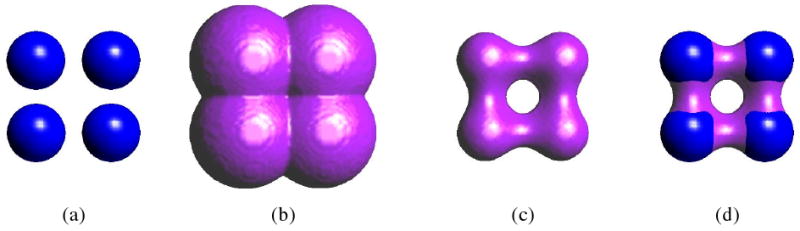
Schematic illustration of the construction algorithm. Figure (a) shows the van der Waals surface for a simple molecule of four atoms. (b) shows the solvent accessible surface defined by φ = 0. (c) shows the solvent excluded surface defined by φ = −1.4. The pink strips in figure (d) show the solvent contact surface where the solvent is taken to be a sphere with radius 1.4.

References

- 1.Osher S, Fedkiw R. Level Set Method and Dynamic Implicit Surfaces. Springer; New York: 2003. [Google Scholar]
- 2.Sethian JA. Cambridge Monographs on Applied and Computational Mathematical. second. Cambridge University Press; 1999. Level Set Methods and Fast Marching Methods: Evolving Interfaces in Computational Geometry, Fluid Mechanics, Computer Visison, and Materials Science. [Google Scholar]
- 3.Osher S, Sethian J. Fronts propagating with curvature-dependent speed: Algorithms based on Hamilton-Jacobi formulations. Journal of Computational Physics. 1988;79:12–49. [Google Scholar]
- 4.Bajaj CL, Xu G, Zhang Q. ICES Report 06-18. Institute for Computational and Engineering Sciences, The University of Texas at Austin; 2006. Smooth Surface Constructions via a Higher-Order Level-Set Method. [Google Scholar]
- 5.Xu G, Zhang Q. Construction of geometric partial differential equations in computational geometry. Mathematica Numerica Sinica. 2006;28(4):337–356. [Google Scholar]
- 6.Osher S, Shu CW. High-order essentially nonoscillatory schemes for Hamilton-Jacobi equations. SIAM Journal of Numerical Analysis. 1991;28(4):907–922. [Google Scholar]
- 7.Peng D, Merriman B, Osher S, Zhao H, Kang M. A PDE-based fast local level set method. Journal of Computational Physics. 1999;155:410–438. [Google Scholar]
- 8.Sanner M, Olson A, Spehner J. Reduced surface: An efficient way to compute molecular surfaces. Biopolymers. 1996;38:305–320. doi: 10.1002/(SICI)1097-0282(199603)38:3%3C305::AID-BIP4%3E3.0.CO;2-Y. [DOI] [PubMed] [Google Scholar]
- 9.Connolly M. Analytical molecular surface calculation. J Appl Cryst. 1983;16:548–558. [Google Scholar]
- 10.Richards FM. Areas, volumes, packing, and protein structure. Ann Rev Biophys Bioeng. 1977;6:151–176. doi: 10.1146/annurev.bb.06.060177.001055. [DOI] [PubMed] [Google Scholar]
- 11.Liang J, Edelsbrunner H, Fu P, Sudhakar PV, Subramaniam S. Analytical shape computation of macromolecules: I. molecular area and volume through Alpha shape. Proteins: Structure, Function, and Genetics. 1998;33:1–17. [PubMed] [Google Scholar]
- 12.Cazals F, Proust F. Revisiting the description of Protein-Protein interfaces. Part I: Algorithms. Research Report 5346, INRIA. 2004 [Google Scholar]
- 13.Cazals F, Proust F. Revisting the description of Protein-Protein interfaces. Part II: Experimental study. Research Report 5501, INRIA. 2005 [Google Scholar]
- 14.Akkiraju N, Edelsbrunner H. Triangulating the surface of a molecule. Discr Appl Math. 1996;71:5–22. [Google Scholar]
- 15.Liang J, Edelsbrunner H, Fu P, Sudhakar PV, Subramaniam S. Analytical shape computation of macromolecules: Ii. inaccessible cavities in protein. Proteins: Structure, Function, and Genetics. 1998;33:18–29. [PubMed] [Google Scholar]
- 16.Blinn J. A generalization of algebraic surface drawing. ACM Transactions on Graphics. 1982;1(3):235–256. [Google Scholar]
- 17.Duncan BS, Olson AJ. Shpae analysis of molecular surfaces. Biopolymers. 1993;33:231–238. doi: 10.1002/bip.360330205. [DOI] [PubMed] [Google Scholar]
- 18.Grant J, Pickup B. A Gaussian description of molecular shape. Journal of Phys Chem. 1995;99:3503–3510. [Google Scholar]
- 19.Zhang Y, Xu G, Bajaj C. Quality meshing of implicit solvation models of biomolecular structures. Computer Aided Geometric Design. 2006;23(6):510–530. doi: 10.1016/j.cagd.2006.01.008. [DOI] [PMC free article] [PubMed] [Google Scholar]
- 20.Baker N, Sept D, Joseph S, Holst M, McCammon J. Proc Natl Acad Sci. USA: 2001. Electrostatics of nanosystems: application to microtubules and the ribosome; pp. 10037–10041. [DOI] [PMC free article] [PubMed] [Google Scholar]
- 21.Holst M, Saied F. Multigrid solution of the Poisson-Boltzmann equation. J Comput Chem. 1993;14:105–113. [Google Scholar]
- 22.Bajaj CL, Djeu P, Siddavanahalli V, Thane A. Texmol: interactive visual exploration of large flexible multi-component molecular complexes. Proceedings of the Annual IEEE Visualization Cnference'04; Austin, Texax, USA. 2004. pp. 243–250. [Google Scholar]
- 23.Zhao H, Osher S, Merriman B, Kang M. Implicit nonparametric shape reconstruction from unorganized points using a variational level set method. Computer Vision and Image Understanding. 2000;80(3):295–319. [Google Scholar]
- 24.Zhao H, Osher S, Fedkiw R. Fast surface reconstruction using the level set method. Proceedings of the IEEE Workshop on Variational and Level Set Methods in Computer Vision (VLSM2001); 2001. pp. 194–201. [Google Scholar]