Nearby boundaries create eddies near microscopic filter feeders

Abstract

We show through calculations, simulations and experiments that the eddies often observed near sessile filter feeders are frequently due to the presence of nearby boundaries. We model the common filter feeder Vorticella, which is approximately 50 µm across and which feeds by removing bacteria from ocean or pond water that it draws towards itself. We use both an analytical stokeslet model and a Brinkman flow approximation that exploits the narrow-gap geometry to predict the size of the eddy caused by two parallel no-slip boundaries that represent the slides between which experimental observations are often made. We also use three-dimensional finite-element simulations to fully solve for the flow around a model Vorticella and analyse the influence of multiple nearby boundaries. Additionally, we track particles around live feeding Vorticella in order to determine the experimental flow field. Our models are in good agreement both with each other and with experiments. We also provide approximate equations to predict the experimental eddy sizes owing to boundaries both for the case of a filter feeder between two slides and for the case of a filter feeder attached to a perpendicular surface between two slides.

1. Introduction

Microscopic sessile filter feeders are an important part of aquatic ecosystems and form a vital link in the transfer of carbon in marine food webs (Fenchel 1982; Sherr & Sherr 1988; Christensen-Dalsgaard & Fenchel 2003; King 2005). The filter feeders consume bacteria and small detritus, and are in turn eaten by larger organisms. Sessile filter feeders live in bodies of water where they are anchored to the stream or ocean bed, aquatic plants or even aquatic animals (Laybourn 1976; Kankaala & Eloranta 1987). They survive by creating a feeding current that draws fluid towards them, and from which they filter their food of interest. These organisms also play an important role in biological waste water treatment (Reid 1969; Chen et al. 2004). An understanding of the flow generated by filter feeders may enable not only a better understanding of marine ecology and carbon cycling, but also improvement of water treatment plant design.

Sessile filter feeders typically have a cell body with a radius ranging from a few to a few hundred microns, and are typically attached either directly or with a stalk to an immobile surface (e.g. an aquatic plant). Some common sessile filter feeders are Vorticella (Sleigh & Barlow 1976), Stentor (Rapport et al. 1972) and choanoflagellates (King 2005). We will focus on Vorticella as a typical sessile filter feeder. Vorticella are a stalked protozoan with a bell-shaped cell body approximately 25 µm across and approximately 50 µm long (Noland & Finley 1931). This body is attached to a surface via a thin stalk of length about 100 µm. Vorticella create a feeding current using a ring of beating cilia at the top of their body, and use two rings of cilia to filter debris from the surrounding fluid (Sleigh & Barlow 1976). The debris can then be ingested into the cell body or rejected into the surrounding fluid (Sleigh & Barlow 1976). There are several possible mechanisms for such particle capture (Rubenstein & Koehl 1977; Labarbera 1984).

Experimental observations of several different sessile filter feeders have shown that they generate feeding currents in the form of a toroidal vortex (Sleigh & Aiello 1972; Sleigh & Barlow 1976; Pettitt et al. 2002; Hartmann et al. 2007; Petermeier et al. 2007; Nagai et al. 2009). Closed feeding streamlines limit the feeder's access to new material (Blake & Otto 1996), so it is important to determine what circumstances lead to closed eddies. The eddy structure is typically attributed to the substrate to which the organism is attached. For instance, Blake & Otto (1996) modelled the feeding eddy structure as a point force, or stokeslet, oriented perpendicular to a plane wall, and this model has been used to estimate feeding fluxes in several biological contexts (Pettitt et al. 2002; Orme et al. 2003; Hartmann et al. 2007).

However, eddies have also been observed near filter feeders even in the absence of a tethering substrate, for instance for a Vorticella attached to a thin strand of duckweed (Sleigh & Barlow 1976) or anchored between two closely spaced parallel slides (Nagai et al. 2009). It seems little recognized that the eddies in these situations, and in fact in the majority of observations of microorganisms, are probably a result of confinement between two walls parallel to the field of view, e.g. the two microscope slides that are nearly universally present when experimentally examining microorganisms (Liron & Blake 1981; Blake et al. 1982).

Liron & Blake (1981) have shown through calculations that closed eddies form only in the presence of boundaries and based on their theoretical calculations suggested that the flow near sessile micro-organisms is mostly determined by the container geometry. They model point-force-generated feeding currents in several geometries, including a stokeslet between two infinite parallel plane boundaries with the stokeslet oriented parallel to the boundaries (Liron & Blake 1981). However, it is difficult to confirm the existence or non-existence of such eddies experimentally, as it is not possible to observe filter feeders under a microscope without introducing at least one nearby boundary.

We build on the calculations of Liron & Blake (1981), and extend them to more complex models of micro-organisms to make experimentally verifiable predictions. We find that the size of the eddies increases approximately linearly with the distance between the confining slides, and emphasize that, according to our calculations and simulations, the eddies disappear entirely for the case of a filter feeder in free space. We then present what we believe is the first experimental confirmation that eddies near filter feeders are due to the boundaries provided by the surrounding slides by showing that the eddy size increases as predicted as the distance between the two confining slides is increased. The origin of these eddies must be taken into account when explaining microscopic filter feeding, as the flow around filter feeders in nature will be quite different from that when examined under a microscope between two slides. We also anticipate that the surroundings of filter feeders, such as whether they have nearby neighbours, will strongly affect the flow nearby, and thus the filter feeder's access to food, oxygen and other nutrients.

2. Stokeslet between two walls

It is common to model sessile filter feeders (and micro-organisms for which gravity is significant) as a point force in Stokes flow—the stokeslet (Blake & Otto 1996; Hartmann et al. 2007; Drescher et al. 2009). Micro-organisms that swim generally do not exert a net force on the surrounding fluid, as the force generated by cilia for swimming is balanced by drag on the organism. However, sessile organisms can apply a net force to the fluid as they are attached (often via a stalk) to a substrate. It is therefore reasonable to approximate such sessile filter feeders using a stokeslet. As the velocity from the stokeslet in free space decays as 1/r, where r is the distance from the stokeslet, and corrections from the details of the body shape and distribution of cilia decay as 1/r² or more rapidly, the stokeslet approximation is likely to be valid far away from the organism. However, if eddies are present in the flow, then their structure may be sensitive to details of the flow close to the organism. In particular, we consider the position of the centre of the eddy, which may be quite close to the organism. It is not clear that a stokeslet model will correctly describe this near-body flow. Here, we compute the position of the stagnation point for a stokeslet between parallel walls, a distance h apart, and in later sections compare it with more realistic models of a filter feeder as well as with experimental results. Note that a list of relevant symbols and their meanings can be found in table 1.

Table 1.

List of symbols used in the main body text in order of appearance.

symbol	physical meaning
r	radial coordinate in cylindrical coordinates
h	distance between no-slip walls in the z direction in experiment, simulation and theory
μ	liquid viscosity
u	liquid velocity field
p	liquid pressure field
rsp	distance between the origin (centre of forcing) and the eddy centre
a	radius of living or model Vorticella depending on context
θ	polar coordinate in cylindrical or spherical coordinates depending on context
ϑ	the co-latitude in cylindrical coordinates ϑ = π −θ
k	permeability used in Brinkman approximation
β	proportionality constant in the definition of k
γE	Euler–Mascheroni constant
ρ	radial coordinate in spherical coordinates
w	width of chamber in simulations
b	length of chamber in simulations
ℓst	the length of the Vorticella stalk
rspl	the eddy size for a sphere located above a single plane boundary

To calculate the flow field, we solve the incompressible Stokes equation and the continuity equation

2.1

We follow Mucha et al. (2004) to numerically calculate the velocity field due to a stokeslet between and parallel to two no-slip walls. For ease of calculation and without affecting the flow near the stokeslet, periodic boundary conditions are imposed on pairs of control surfaces orthogonal to the bounding walls and far from the stokeslet (see figure 1a for a schematic view). We set the width and length of the periodic boundaries (in the x and y directions) to be much larger than the distance, h, between the no-slip walls, such that the eddy structure is determined by the no-slip walls. The stokeslet is located in the mid-plane at (0, 0, h/2) and points in the −e_y direction. Details of the calculation are found in appendix A. We note that an alternative calculation for a stokeslet between infinite parallel walls can be found in Liron & Mochon (1976).

Figure 1.

(a) Stokeslet between parallel walls. The stokeslet is represented by a grey arrow pointing in the −e_y direction and the dotted lines represent periodic boundaries. The upper and lower boundaries (parallel to the x−y plane) are no-slip. (b) Brinkman approximation geometry. (c) Simulation geometry. The upper and lower boundaries are no-slip. The right-hand and left-hand boundaries are open, and the front and back boundaries are slip. (d) A schematic view of the experimental set-up. Vorticella are grown on the narrow edge of a glass coverslip (grey box), which is inserted midway between two slides, a distance h apart.

Previous discussions of the eddies generated by a stokeslet between parallel plates have approximated the flow as generated by a potential dipole (Liron & Blake 1981; Blake et al. 1982). In this limit, it is not possible to make an approximation for the position of the eddy centres, as for a point dipole all streamlines share a common tangent at the position of the dipole, and both eddy centres are located at the position of the dipole. Instead of making such an approximation, we calculate the full solution to the Stokes equation in the near field. This approach allows us to find the position of the centre of the eddy. The flow is symmetric around the axis of the stokeslet (figure 2a), such that the stagnation point at the centre of the eddy in the z = h/2 plane is located on the x-axis. As all length scales can be non-dimensionalized by h, we find that the distance to the stagnation point, r_sp, at the centre of the eddy increases linearly with the distance between the no-slip plane boundaries. In fact, from the numerically computed streamlines near the stokeslet (figure 2), we find r_sp/h = 0.44 ± 0.01.

Figure 2.

Streamlines in the mid-plane for different filter-feeder models. (a) Stokeslet model from §2 scaled by h. (b) Brinkman symmetric model from §3 with h = 2.5a and k = (h/a)². (c) Brinkman asymmetric model from §3 with h = 2.5a and k = (h/a)². (d) Simulation from §4 with h = 2.5a.

3. Brinkman approximation

The stokeslet approximation described in §2 does not take the finite size of the feeding organism into account, or the distribution of the cilia that maintain continuous circulation of the fluid. The detailed geometry of the cell body may significantly affect the flow field near to the organism (Sleigh & Aiello 1972). In this section, we exploit the narrow-gap geometry of the feeding currents to introduce an approximation that can handle the finite-sized cell body.

We treat the feeding organism as a cylinder, of radius a, between two closely spaced walls as shown in figure 1b. For ease of comparison, rather than using the customary polar coordinate angle θ, we define the co-latitude ϑ = π−θ (figure 1b), and write all equations of motion in terms of r and ϑ. Together, r, ϑ and −z form a right-handed coordinate system. We model the generation of a feeding current by cilia distributed over the cell body by prescribing a tangential velocity u_ϑ. A similar method of prescribing tangential velocity has been used to model swimming micro-organisms (Magar et al. 2003; Ishikawa & Pedley 2008). Surface-generated flows around swimming Volvox have been represented in a functionally similar manner using a prescribed tangential stress boundary condition (Short et al. 2006). In order to show the effect of the distribution of cilia on the cell body upon the flow streamlines, we consider two different velocity distributions at r = a (figure 3). The first, or symmetric, model has u_ϑ = u₀ sin ϑ at r = a, which we assume models a symmetric distribution of cilia on the surface pushing fluid tangentially with typical speed u₀. The second type of boundary condition is intended to capture the fact that cilia are concentrated near the top of the organism in a ‘crown’, as is true of many filter feeders, including Vorticella. For this asymmetric model, we have at r = a

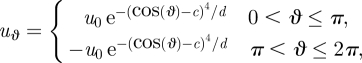3.1

where we choose c = 1/2 and d = 1/100 to provide a localized surface forcing and where variables are dimensional for the moment. The two cases account for the change in direction of e_ϑ so that the final velocity is symmetric across the y-axis. In both models, u_r = 0 at r = a so that there is no flow through the cylinder surface.

Figure 3.

The non-dimensional velocity, u_ϑ, at r = 1, the surface of the cylinder, for the symmetric (dashed line) and asymmetric (solid line) Brinkman models.

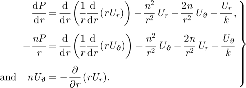
To calculate the flow, we solve equation (2.1) non-dimensionalized by scaling all lengths by a, velocities by u₀ and stresses by µu₀/a. We also specify u = e_ϑu_ϑ on r = 1 and no-slip conditions on all other rigid boundaries (z = ±(1/2)(h/a)), with the flow vanishing at infinity. Finally, we work under the Brinkman approximation (Brinkman 1947; Tsay & Weinbaum 1991; Fernandez et al. 2002) for the variation of the flow across the gap, which gives: ∂²u/∂z² = −(u/k), where k ∝ (h/a)² is the permeability, and the velocity is restricted to planes parallel to the boundaries, i.e. u = (u_r, u_ϑ) and u_z ≡ 0. In addition to modifying the usual Hele–Shaw flow law to include the viscous effect of flow variations parallel to the cover slips (Fernandez et al. 2002), the Brinkman approximation allows both normal and tangential velocity boundary conditions to be applied on the surface of the cylinder. We expect that the velocity decays as r → ∞. The r and ϑ components of this equation give, respectively,

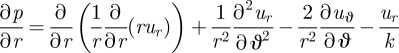3.2

and

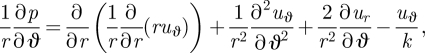3.3

and the continuity equation is

3.4

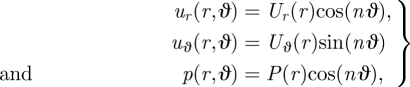
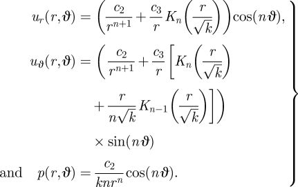
In appendix B, we derive the general solution to this system of equations. In particular, given the generic boundary condition u_ϑ = sin nϑ on the surface of the cylinder, the velocity and pressure fields take the form

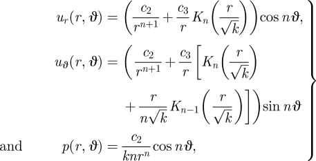3.5

where K_n are the modified Bessel functions of the second kind and, for some pair of constants c₂ and c₃, that must be determined from the boundary conditions. At r = 1, we have u_r = 0 and u_ϑ = sin nϑ for all ϑ and k. Hence, we find

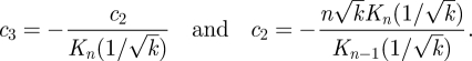3.6

Setting n = 1 in equations (3.5) and (3.6) gives a solution for the symmetric model filter feeders.

To create the ‘crown of cilia’ boundary condition, we use a Fourier series u_ϑ = ∑₁^∞ A_n sin(nϑ) with A_n = (2/π)∫₀^πe^{(−(cos(ϑ)−c)4/d)} sin (nϑ) dϑ with c and d as defined earlier. We find that 25 terms in this series are required to limit error in the boundary condition to less than 1 per cent (the 25-term sum is plotted in figure 3). Streamlines for both cases are shown in figure 2.

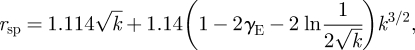
We define the size of the eddy, r_sp, as the distance from the centre of the cylinder to the stagnation point at the centre of the eddy (scaled by a). This distance is numerically calculated by finding the point where u_ϑ = u_r = 0. In the symmetric case, this point falls on the x-axis (ϑ = π/2). In both cases, the eddy size increases with the spacing between the confining walls (see figure 4 where we have now scaled r_sp by h rather than a). To determine the dependence of eddy size upon the gap width, we define k = β(h/a)², where β is a proportionality constant. We plot the cases β = 1/12 in figure 4, which is the value for pressure-driven flow in a Hele–Shaw cell without obstacles and also the case β = 0.16, which gives an exact match between the value for r_sp for the stokeslet and the asymptotic value of r_sp in the Brinkman geometry at a/h = 0. We can analytically evaluate the contribution of the finite-sized cell body to the size of the eddy when h ≫ a. For large k, asymptotic analysis (appendix B) gives , where γ_E is the Euler–Mascheroni constant (we now explicitly write the non-dimensionalization for clarity). For comparison, in figure 4, we also show r_sp for a stokeslet between parallel plates as a single point with a/h = 0. We also note that the first term in the asymptotic expansion gives r_sp ∝ h, which is the same scaling result as from the stokeslet model in §2.

Figure 4.

Eddy size for several different models of a filter feeder. Large open circle (white), stokeslet between parallel plates. Asterisks, Brinkman symmetric model; open circles, Brinkman asymmetric model; solid line, Brinkman symmetric model expansion as detailed in the text for a/h → 0. For the Brinkman model, grey symbols correspond to the best fit value β = 0.16 and black to the Hele–Shaw approximation β = 1/12. Filled circles, three-dimensional simulation (§4). Open rectangle (dark grey), experimental observations; error bars show 95% confidence interval.

We have simplified the full three-dimensional flow generated by the filter feeder to a two-dimensional model. This approach is a good first step in finding an analytical solution to the problem, and retains features from the stokeslet solution including an eddy size that increases with the separation between the no-slip boundaries. We expect the Brinkman equations to accurately model the true flow field, provided that the dimensionless permeability k > 5 (Tsay & Weinbaum 1991), i.e. when the gap thickness, h ∼ 5.6a for β = 0.16. We expect this condition to be fulfilled in most experimental situations. However, the approximate nature of the boundary conditions applied at the feeder surface means that there may yet be quantitative differences between our Brinkman cylindrical model and the true three-dimensional flow field. We check for this in §4 using finite-element simulations to solve the full three-dimensional flow problem for a spherical cell body between two no-slip boundaries.

4. Three-dimensional simulations

In order to analyse the effect of the approximations that were introduced in the Brinkman model and to model the influence of additional nearby boundaries upon the eddy size, we solve the full three-dimensional incompressible Stokes equation using finite-element analysis with Comsol Multiphysics software. We compare our simulations both with flow currents visualized in real filter feeders and with the predictions of the Brinkman model. To simulate the full three-dimensional flow field, we represent the three components of the velocity field by second-order elements, and use linear elements for the pressure field, p. The geometry for the simulation is shown in figure 1c. On the sphere, we specify u_θ = sin θ and u_ρ = 0 where ρ and θ are spherical variables measured from the y-axis as shown in figure 1c. Although we have used θ here in a slightly different definition from that in the two-dimensional calculation, we do not anticipate any confusion from the reader. The glass slides are represented by upper and lower no-slip boundaries. The right-hand and left-hand boundaries are open, and slip conditions are applied on the front and back boundaries, making the system periodic in this direction. We adjust the width of the chamber, w, and its length, b, to ensure that the effect of chamber size on the eddy radius is less than 1 per cent.

The eddy centre is found numerically by finding the location in the z = h/2 plane where u = 0 (velocities are interpolated between nodes using cubic patches). Typical results are plotted in figure 4. Realistic boundary conditions produce feeding loci that agree very well with our new analytical results, even when a ≈ h/2, so that the feeder almost touches the top and bottom plates. We note that the three-dimensional simulation results, which have a symmetric boundary condition, quantitatively match best the asymmetric Brinkman flow result, but in trend match best the symmetric Brinkman flow result.

5. Experimental results

Experimental observations of closed eddies around the filter feeder Vorticella convallaria confirm predictions from our models. In our experiments, V. convallaria are cultured as in Ryu & Matsudaira (submitted) and transferred to a Petri dish for observation under the microscope (Leica DMIRM, 10× magnification). To trace the flow, the fluid near the V. convallaria of interest is seeded with 1 µm diameter polystyrene beads, and the motion of these beads is filmed at 100 frames per second. Similar flow-field measurements have been made but the effect of changing boundaries was not examined (Sleigh & Aiello 1972; Sleigh & Barlow 1976; Nagai et al. 2009).

We probe the effect of two different boundary configurations upon the eddies generated by the filter feeder. First, we observe V. convallaria anchored to the edge of a coverglass (Corning Labware and Equipment no. 1) between two slides, as illustrated schematically in figure 1d. The distance between slides, h, is varied from 140 ± 20 to 566 ± 28 µm. In a second set-up, we observe V. convallaria between two slides, a distance h = 127 ± 28 µm apart, with the Vorticella midway between the two slides and without the presence of an anchoring coverslip. In this configuration, the Vorticella stalk is anchored to the bottom slide, but bent so that the Vorticella body has the same orientation relative to the slides as in figure 1d. This situation is most analogous to our calculations and simulations because the only boundaries present are the top and bottom no-slip slide surfaces.

We use particle tracking velocimetry (PTV) software custom-written in Matlab to extract flow-field data from videos of feeding V. convallaria. Particles are tracked using PolyParticleTracker in Matlab using the method of Rogers et al. (2007). Velocities are then calculated from the displacement of particles between sequential frames. These velocities are then binned in the x and y directions, the velocities in each bin averaged and this average velocity assigned to the centre of the bin. While there are some areas where we cannot compute the velocity owing to lack of particles tracked (often near the centre of the eddy), we find that this method creates reliable flow fields for most of our data. We re-scale these data by dividing lengths by the radius of V. convallaria (determined as the maximum width of the V. convallaria body in the first video frame) and rotate tracks so that the long axis of the V. convallaria body is aligned with the y-axis for ease of comparison with calculations and simulations. We also centre the tracks so that the centre of the V. convallaria is at (0, 0) in the x–y plane.

The centres of the eddies are found based on an algorithm similar to that described in §4, where the velocity data are interpolated when necessary. An example of the full data analysis process is shown in figure 5.

Figure 5.

An example of the analysis of experimental data. (a) One frame from a high-speed movie showing a V. convallaria in the centre overlayed with particle tracks. The Vorticella body is outlined in a thick solid line. Scale bar, 100 µm. (b) The particle tracks from (a) rotated and scaled by the radius of the Vorticella. The circles show the position and radius of the Vorticella. (c) The flow field calculated by PTV. Velocities are scaled such that they will not intersect, and then lengthened by a further factor of four. The three largest velocity vectors have been removed for ease of viewing. X-marks surrounded by circles (grey) show the centre of the eddies with the outer circle representing the positional error. For this example, h = 127 ± 28 µm.

In the experimental situation most analogous to our calculations and simulations, with the Vorticella midway between two slides and with h = 127 ± 28 µm, we find r_sp/h = 0.48 ± 0.06 (95% confidence interval, N = 10). This point is plotted in figure 4 for comparison with calculations and simulations. We find that this experiment agrees with the Brinkman model, confirming that the eddies seen in these experiments are due to the confining boundaries of the two slides parallel to the plane of view.

For our experiments where the Vorticella is anchored to the narrow side of a coverglass, as in figure 1d, the presence of this anchoring boundary must be taken into account in addition to the boundaries above and below the Vorticella. For this reason, we repeat the simulations as in §4, with the geometry modified so that there is a third no-slip boundary at y = −ℓ_st, where the length ℓ_st represents the length of the Vorticella stalk. In our experiments, this length ranges from ℓ_st/a ≈ 3 to 5. The geometry for the simulation is shown in figure 6.

Figure 6.

Simulation geometry for comparison with experiments. The upper and lower boundaries are no-slip. The right-hand and left-hand boundaries are open, and the front boundary is slip. The back boundary is no-slip, we emphasize this change from figure 1c by shading this boundary grey. This diagram is not to scale. In simulations and experiments, a < ℓ_st ≪ w,b.

In order to collapse the eddies from cells at different sizes, with different coverglass separations, and different stalk lengths, we scale the eddy sizes measured from experiments and simulations by the eddy size, r_sp^l, for a sphere located above a single-plane boundary at y = −ℓ_st, with the boundary condition of §4 imposed on the sphere and no additional boundaries present (figure 8). In the limit ℓ_st/h < 1, asymptotic analysis gives r_sp^l/ℓ_st = 1.085 + 4.705(a/ℓ_st)² (see appendix C).

When scaled appropriately, experimental and simulated data agree over a wide range of different cell body sizes, as shown in figure 7, which demonstrates that the size of the feeding eddies is controlled by the confining walls through which the flows are observed.

Figure 7.

Plot of r_sp/r_sp^l versus h/r_sp^l for simulations (shapes) and experiments (circles), where r_sp^l is the predicted distance to the eddy centre for large h as described in the text. The solid line is the prediction r_sp = 0.44 h from the stokeslet model. In experiments, ℓ_st was measured from the anchoring tip of the Vorticella stalk to the middle of the crown. In simulations, both h, the distance between top and bottom boundaries, and ℓ_st, the distance to the third no-slip boundary, were varied. Squares: h/a = 2.5–40, ℓ_st/a = 3; diamonds: h/a = 2.5–40, ℓ_st/a = 10; upward triangles: h/a = 3, ℓ_st/a = 1.5–50; downward triangles: h/a = 10, ℓ_st/a = 1.5–50.

Figure 8.

Schematic of geometry for sphere above plane boundary calculations. Dotted line represents an axis of symmetry.

From figure 7, we can see that, for h < r_sp^l, the eddy size is well predicted by the stokeslet model, r_sp = 0.44 h (shown as a solid line in figure 7). On the other hand, for h ∼ r_sp^l, the eddy size is well predicted by a model that accounts for the new no-slip boundary but neglects all other boundaries. In general, although we would intuitively expect that the eddy size is controlled by the distance to the closest boundary, it seems that the system actually selects the smallest of the two possible eddy sizes (either from the anchoring wall or from the coverslips).

The large error bars on the experimental data are owing to errors inherent in measuring and centring the V. convallaria in digital images as well as to the interpolation necessary to locate the centres of these eddies. There is also some error in determining the distance between slides, h, which arises mainly from variation in manufacturing of the spacers that we use (either coverglasses of varying thickness, or paper spacers from the Hybaid EasiSeal system). We also do not account for drift of the Vorticella body out of the mid-plane, or for tilting of the body with respect to the tethering coverglass, although experiments were discarded if during filter feeding the Vorticella crown was pointed in the ±e_z direction. We believe that these variations account for most of the quantitative discrepancy between simulation and theory in figure 7. This leaves only a small residue of difference between the experimental measurements and the predictions of the model that must be attributed to the unmodelled effects of cell-body geometry and the location of the bands of cilia in real Vorticella.

6. Conclusion

We have derived and validated a hierarchy of models for the flow created by Vorticella between two parallel walls. Three-dimensional finite-element simulations agree in detail with the experiment. In the absence of an anchoring wall, as for instance when the cell is tethered to either of the coverslips, a Brinkman flow model is in good agreement with the simulations, and provides an analytically tractable method for determining the effect of cell shape, and of the placement of cilia of the Vorticella upon the feeding currents.

We also explored a common experimental scenario, in which Vorticella is anchored to a wall, which provides a third confining boundary, in addition to the parallel boundaries representing the coverslips. Although in general all three nearby boundaries must be considered, we found that, over a wide range of experimental conditions, the two sets of boundaries produce eddies that are well separated in size. For this situation, the eddy size is determined by the minimum of the eddy sizes predicted when the two sets of boundaries are considered separately. Only when the two sets of boundary conditions independently give rise to eddies of approximately the same size must all boundaries be considered together when predicting the eddy size.

For experimentalists studying the flow around microscopic sessile filter feeders, caution should be used when observing closed feeding currents near boundaries. It is likely that these eddies are caused by the fact that the organism is applying a force to the fluid near a boundary and not by any particular motion of the organism under observation. As a guide to such experiments, we summarize the results of this work as a rule of thumb. For a sessile filter feeder anchored to a boundary perpendicular to the plane of view, eddies caused by boundaries will have a size approximately

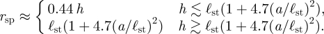6.1

Without the presence of a perpendicular boundary, eddies caused by boundaries will have a size of approximately 0.44 h. Only eddies of different length scales from those predicted above are likely to be caused by the specific action of the organism under observation. In particular, the distance between the organism and the coverslips through which the flow is observed should be at least 2.3 times the size of any observed eddy to ensure that the eddy is not a boundary artefact.

We have shown that the flow around filter feeders in nature will be quite different from that when examined under a microscope between two slides. Single filter feeders in nature may have much greater access to nutrients than predicted from experiments. For instance, observations of flow volumes and rates based on experiments in confined geometries (Sleigh & Barlow 1976; Nagai et al. 2009) are likely to significantly underestimate the values of such parameters in nature.

Although we have discussed the role of geometric confinement as a confounding factor when comparing experimentally observed feeding flows with the flow structures created by filter-feeding organisms in their natural environments, boundary-dominated flows may yet exist in nature. Filter feeders may find themselves either confined by the substrate to which they are anchored or crowded by neighbouring feeders. In general, nearby surroundings will strongly affect the flow generated by the filter feeder, and thus the feeding efficiency of the organism.

Appendix A: Stokeslet between parallel walls with periodic boundary conditions

We follow Mucha et al. (2004) to numerically calculate the velocity field owing to a stokeslet between and parallel to no-slip walls with periodic boundary conditions (see figure 1a for a schematic view). The walls are separated by a distance, h, with a periodic length of w and b in the x and y directions, respectively. The stokeslet is located at (0, 0, Z) and points in the e_y direction; we will later specify Z = h/2 to analyse the flow due to a stokeslet in the mid-plane.

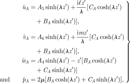
The velocity, U = (u, v, w), is expanded in a Fourier series in the x and y directions, U(r) = ∑_λÛ(z)exp (iℓx + imy) with the summation over λ = (ℓ, m). The expansion in the Stokes equation yields

A 1

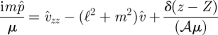A 2

A 3

where µ is the viscosity of the fluid and 𝒜 is the periodic area, w × b. The continuity equation gives

A 4

We also specify Û = 0 at z = 0 and z = h. Summing the z-derivative of equation (A 3) with equation (A 1) multiplied by iℓ and equation (A 2) multiplied by im and combining and eliminating the velocities using the continuity equation gives

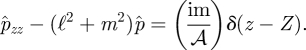A 5

This equation can be solved separately in the regions above and below the stokeslet. Below the stokeslet (0 < z < Z), we find

A 6

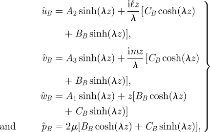
where 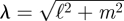and where we have used the velocity boundary condition to eliminate some terms. Combining the above with the continuity equation gives B_B = −λA₁, C_B = −iℓA₂ − imA₃. Above the stokeslet (Z < z < h), we find

A 7

where z′ = h − z, and we have used the velocity boundary condition at z = h. Combining the above with the continuity equation, as before, gives B_A = λA₄, C_A = −iℓA₅ − imA₆. We next find the A_j coefficients by satisfying the conditions at z = Z: û, v̂, ŵ and p̂ are continuous. We also find, by integrating equations (A 1)–(A 3) and (A 5), that û_z and ŵ_z are continuous while v̂_Az(Z)–v̂_Bz(Z) = −1/(𝒜µ) and p̂_Az(Z) − p̂_Bz (Z) = im/𝒜. We can solve for the A_j for a given λ and Z by combining these jump conditions with equations (A 6) and (A 7). The algebraic equations for the A_j can be found in table 1 of Mucha et al. (2004), with a change of variables (d → h, X → Z, η → µ and k → λ) to match the coordinates and conventions of our paper. Note that we believe there is a typographical error in Mucha et al. (2004) eqn (A 9) and that the equation for A₆ should be −2 multiplied by the current equation.

Appendix B: Details of Brinkman flow calculations

To calculate the flow around a cylinder of radius a as in figure 1b, we solve the boundary value problem

B 1

where we have scaled all lengths by a, velocities by u₀ and stresses by μu₀/a. For convenience, we define ϑ = π–θ. We also specify the boundary condition at r = 1 of u_ϑ = sin(nϑ), where n ≥ 1 and is an integer, u_r = 0, and no-slip conditions on all other rigid boundaries (z = ±(1/2)(h/a)) and at infinity. We work under the Brinkman approximation (Brinkman 1947; Tsay & Weinbaum 1991), which here amounts to ∂²u/∂z² = −(u/k), where k ∝ (h/a)² is the permeability and the velocity is restricted to planes parallel to the boundaries, i.e. u = (u_r, u_ϑ) and u_z ≡ 0. In a component form, we have

B 2

and the continuity equation is

B 3

Equations (B 2) and (B 3) are unchanged with the substitutions u_θ → u_ϑ and ∂/∂θ → ∂/∂ϑ as u_θ = −u_ϑ and ∂/∂θ = −(∂/∂ϑ). Because of the form of the boundary conditions, we then seek

B 4

which reduce the governing equations to

B 5

With a little algebra, we can eliminate U_ϑ and P in order to arrive at a single fourth-order ordinary differential equation for U_r

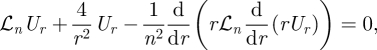B 6

where the operator ℒ_n is defined as ℒ_n = (d/dr)((1/r) (d/dr)(r·)) − (n²/r²) − (1/k). The solution of this equation is

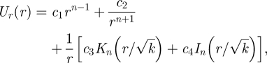B 7

where I_n and K_n are modified Bessel functions of order n. In order for the solution to be bounded as r → ∞, we take c₁ = c₄ = 0.

From the continuity equation, we find U_ϑ(r) and from equation (B 2) we obtain the pressure field. Putting the details together, we have

B 8

At r = 1, we have u_r = 0 and u_ϑ = sinϑ for all ϑ and k. Hence, we find

B 9

We next evaluate the stream function for the motion in the plane. For cylindrical coordinates,

B 10

We then integrate the equations above to obtain

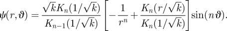B 11

The streamlines for the n = 1 case are plotted in figure 2b.

We also find the position of the eddy centre as k approaches ∞. The limiting behaviour of the modified Bessel function, K_n(x), for x ≪ 1 is (Jackson 1998)

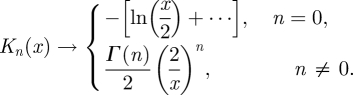B 12

From equation (B 8), we see that u_r = 0 when ϑ = π/2, i.e. on the x-axis for all odd n. For odd n, the eddy centre lies on the x-axis at a radial position that satisfies

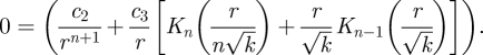B 13

In the limit k ≫ 1 we find . Defining , equation (B 13) reduces to

B 14

in the k ≫ 1 limit, giving the position of the eddy centre at

B 15

We numerically find that, for n = 1, the symmetric boundary condition case, s = 1.114, satisfies equation (B 14). Further expansion of equation (B 13) for n = 1 gives a two-term approximation for the position of the eddy centre of

B 16

where γ_E is the Euler–Mascheroni constant. Substituting k = β(h/a)², where β is a proportionality constant, and using dimensional variables yields

B 17

which is plotted in figure 4 for two values of β.

Appendix C: Sphere above a plane boundary

To calculate the flow around a sphere with radius a above a plane boundary as in figure 8, we solve the boundary value problem

C 1

where we have scaled all lengths by a, velocities by u₀ and stresses by μu₀/a. We work in spherical coordinates with the sphere centred on the origin and the wall at y = −ℓ_st. We enforce on the surface of the sphere (ρ = 1) u_ρ = 0 and u_θ = sinθ and at the wall u = 0. We simplify the solution by noting that, in free space, a sphere with the above boundary conditions consists of a superposition of a stokeslet pointing in the −e_y direction and a point dipole of equal strength pointing in the opposite direction, both located at the centre of the sphere. Therefore, a sphere next to a plane with these boundary conditions can be approximated by superposing a stokeslet and its image system with a point dipole and its image system.

In this section, we will work with the stream functions in spherical axially symmetric coordinates for simplicity. In these coordinates, we have

C 2

and equation (C 1) reduces to E⁴ψ = 0, where E⁴ = E² ∘ E² and

C 3

A stokeslet at the origin oriented in −e_y direction gives

C 4

The potential dipole can be derived as (Chwang & Wu 1975, p. 791) yielding

C 5

For a sphere with boundary condition u_θ = sinθ we have

C 6

We must now consider the image system for these singularities. The solution for a stokeslet above a no-slip boundary is well known to be the solution for the original stokeslet in free space plus an image system consisting of a stokeslet, a source dipole and a stokeslet doublet (Blake 1971; Blake & Chwang 1974; Pozrikidis 1992)

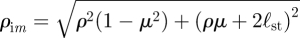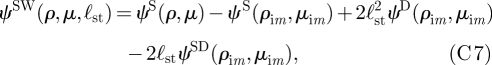
where we use μ = cosθ for convenience and where is the radial distance measured from the image position and 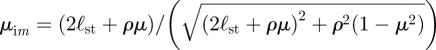is based on the angle measured from the image position. The images are located on the axis at y = −2ℓ_st. Similarly, the stream function for a potential dipole above a wall is

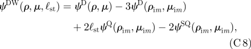where ψ^Q and ψ^SQ are the stream functions for a potential quadrupole and Stokes quadrupole, respectively, and

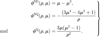C 9

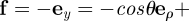
The above equations can be derived from equations (C 4) and (C 5) by noting that the next multipole/multiplet in the series can be derived by taking (f · ∇)ψ, where ψ is the previous multipole/multiplet and f is the unit direction of the new multipole/multiplet (Chwang & Wu 1975). For instance, . In our case and

For a sphere of radius ρ = 1 at height ℓ_st above a no-slip wall with u_θ = 0 and u_ρ = 0 at the surface of the sphere, we have an approximation of

C 10

where

C 11

This approximation satisfies the no-slip boundary condition at y = −ℓ_st without error, but has errors of order 1/ℓ_st and (1/ℓ_st)² for u_ρ and u_θ, respectively, on the surface of the sphere, which could be corrected by adding further image terms.

To find the position of the eddy centre, r_sp^l, we solve two simultaneous equations u_ρ = 0 and u_θ = 0. The velocity components can be calculated by combining equation (C 2) with equation (C 10). While these equations are complex, they yield a simple asymptotic expansion for 1/ℓ_st≪1,

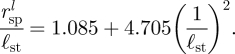C 12

References

- Blake J. R. 1971. A note on the image system for a stokeslet in a no-slip boundary. Math. Proc. Camb. Philos. Soc. 70, 303–310. ( 10.1017/S0305004100049902) [DOI] [Google Scholar]
- Blake J., Chwang A. 1974. Fundamental singularities of viscous flow. J. Eng. Math. 8, 23–29. ( 10.1007/BF02353701) [DOI] [Google Scholar]
- Blake J. R., Otto S. R. 1996. Ciliary propulsion, chaotic filtration and a ‘blinking’ stokeslet. J. Eng. Math. 30, 151–168. ( 10.1007/BF00118828) [DOI] [Google Scholar]
- Blake J. R., Liron N., Aldis G. K. 1982. Flow patterns around ciliated microorganisms and in ciliated ducts. J. Theor. Biol. 98, 127–141. ( 10.1016/0022-5193(82)90062-5) [DOI] [PubMed] [Google Scholar]
- Brinkman H. C. 1947. A calculation of the viscosity and the sedimentation constant for solutions of large chain molecules taking into account the hampered flow of the solvent through these molecules. Physica 13, 447–448. ( 10.1016/0031-8914(47)90030-X) [DOI] [Google Scholar]
- Chen S., et al. 2004. The activated-sludge fauna and performance of five sewage treatment plants in Beijing, China. Eur. J. Protistol. 40, 147–152. ( 10.1016/j.ejop.2004.01.003) [DOI] [Google Scholar]
- Christensen-Dalsgaard K. K., Fenchel T. 2003. Increased filtration efficiency of attached compared to free-swimming flagellates. Aquat. Microb. Ecol. 33, 77–86. ( 10.3354/ame033077) [DOI] [Google Scholar]
- Chwang A. T., Wu T. Y. T. 1975. Hydromechanics of low-Reynolds-number flow. Part 2. Singularity method for Stokes flows. J. Fluid Mech. 67, 787–815. ( 10.1017/S0022112075000614) [DOI] [Google Scholar]
- Drescher K., Leptos K. C., Tuval I., Ishikawa T., Pedley T. J., Goldstein R. E. 2009. Dancing volvox: hydrodynamic bound states of swimming algae. Phys. Rev. Lett. 102, 168101 ( 10.1103/PhysRevLett.102.168101) [DOI] [PMC free article] [PubMed] [Google Scholar]
- Fenchel T. 1982. Ecology of heterotropic microflagellates. IV. Quantitative occurrence and importance as bacterial consumers. Mar. Ecol. Prog. Ser. 9, 35–42. ( 10.3354/meps009035) [DOI] [Google Scholar]
- Fernandez J., Kurowski P., Petitjeans P., Meiburg E. 2002. Density-driven unstable flows of miscible fluids in a Hele–Shaw cell. J. Fluid Mech. 451, 239–260. [Google Scholar]
- Hartmann C., Ozlemzmutlu O., Petermeier H., Fried J., Delgado A. 2007. Analysis of the flow field induced by the sessile peritrichous ciliate Opercularia asymmetrica. J. Biomech. 40, 137–148. ( 10.1016/j.jbiomech.2005.11.006) [DOI] [PubMed] [Google Scholar]
- Ishikawa T., Pedley T. J. 2008. Coherent structures in monolayers of swimming particles. Phy. Rev. Lett. 100, 088103 ( 10.1103/PhysRevLett.100.088103) [DOI] [PubMed] [Google Scholar]
- Jackson J. D. 1998. Classical electrodynamics, p. 116, 3rd edn New York, NY: Wiley. [Google Scholar]
- Kankaala P., Eloranta P. 1987. Epizooic ciliates (Vorticella sp.) compete for food with their host Daphnia longispina in a small polyhumic lake. Oecologia 73, 203–206. ( 10.1007/BF00377508) [DOI] [PubMed] [Google Scholar]
- King N. 2005. Choanoflagellates. Curr. Biol. 15, R113–R114. ( 10.1016/j.cub.2005.02.004) [DOI] [PubMed] [Google Scholar]
- Labarbera M. 1984. Feeding currents and particle capture mechanisms in suspension feeding animals. Am. Zool. 24, 71–84. [Google Scholar]
- Laybourn J. 1976. Energy budgets for Stentor coeruleus Ehrenberg (Ciliophora). Oecologia 22, 431–437. ( 10.1007/BF00345319) [DOI] [PubMed] [Google Scholar]
- Liron N., Blake J. R. 1981. Existence of viscous eddies near boundaries. J. Fluid Mech. 107, 109–129. [Google Scholar]
- Liron N., Mochon S. 1976. Stokes flow for a stokeslet between two parallel flat plates. J. Eng. Math. 10, 287–303. ( 10.1007/BF01535565) [DOI] [Google Scholar]
- Magar V., Goto T., Pedley T. J. 2003. Nutrient uptake by a self-propelled steady squirmer. Quart. J. Mech. Appl. Math. 56, 65–91. ( 10.1093/qjmam/56.1.65) [DOI] [Google Scholar]
- Mucha P. J., Tee S. Y., Weitz D. A., Shraiman B. I., Brenner M. P. 2004. A model for velocity fluctuations in sedimentation. J. Fluid Mech. 501, 71–104. ( 10.1017/S0022112003006967) [DOI] [Google Scholar]
- Nagai M., Oishi M. I., Oshima M., Asai H., Fujita H. 2009. Three-dimensional two-component velocity measurement of the flow field induced by the Vorticella picta microorganism using a confocal microparticle image velocimetry technique. Biomicrofluidics 3, 014105 ( 10.1063/1.3105106) [DOI] [PMC free article] [PubMed] [Google Scholar]
- Noland L. E., Finley H. E. 1931. Studies on the taxonomy of the genus Vorticella. Trans. Am. Micros. Soc. 50, 81–123. ( 10.2307/3222280) [DOI] [Google Scholar]
- Orme B. A. A., Blake J. R., Otto S. R. 2003. Modelling the motion of particles around choanoflagellates. J. Fluid Mech. 475, 333–355. [Google Scholar]
- Petermeier H., Kowalczyk W., Delgado A., Denz C., Holtmann F. 2007. Detection of microorganismic flows by linear and nonlinear optical methods and automatic correction of erroneous images artefacts and moving boundaries in image generating methods by a neuronumerical hybrid implementing the Taylor's hypothesis as a priori knowledge. Exp. Fluids 42, 611–623. ( 10.1007/s00348-007-0269-3) [DOI] [Google Scholar]
- Pettitt M. E., Orme B. A. A., Blake J. R., Leadbeater B. S. C. 2002. The hydrodynamics of filter feeding in choanoflagellates. Eur. J. Protistol. 38, 313–332. ( 10.1078/0932-4739-00854) [DOI] [Google Scholar]
- Pozrikidis C. 1992. Boundary integral and singularity methods for linearized viscous flow, pp. 22 and 84 Cambridge, UK: Cambridge University Press. [Google Scholar]
- Rapport D. J., Berger J., Reid D. B. W. 1972. Determination of food preference of Stentor coeruleus. Biol. Bull. 142, 103–109. ( 10.2307/1540249) [DOI] [Google Scholar]
- Reid R. 1969. Fluctuations in populations of 3 Vorticella species from an activated-sludge sewage plant. J. Protozool. 16, 103–111. [DOI] [PubMed] [Google Scholar]
- Rogers S. S., Waigh T. A., Zhao X., Lu J. R. 2007. Precise particle tracking against a complicated background: polynomial fitting with Gaussian weight. Phys. Biol. 4, 220–227. ( 10.1088/1478-3975/4/3/008) [DOI] [PubMed] [Google Scholar]
- Rubenstein D. I., Koehl M. A. R. 1977. The mechanisms of filter feeding: some theoretical considerations. Am. Nat. 111, 981–994. ( 10.1086/283227) [DOI] [Google Scholar]
- Ryu S., Matsudaira P. T. Submitted Unsteady motion, finite reynolds number and wall effects on Vorticella convallaria contribute contraction force greater than the stokes drag. Biophys. J. [DOI] [PMC free article] [PubMed] [Google Scholar]
- Sherr E., Sherr B. 1988. Role of microbes in pelagic food webs: a revised concept. Limnol. Oceanogr. 33, 1225–1227. [Google Scholar]
- Short M. B., Solari C. A., Ganguly S., Powers T. R., Kessler J. O., Goldstein R. E. 2006. Flows driven by flagella of multicellular organisms enhance long-range molecular transport. Proc. Natl Acad. Sci. USA 103, 8315–8319. ( 10.1073/pnas.0600566103) [DOI] [PMC free article] [PubMed] [Google Scholar]
- Sleigh M. A., Aiello E. 1972. The movement of water by cilia. Acta Protozool. 11, 265–277. [Google Scholar]
- Sleigh M. A., Barlow D. 1976. Collection of food by Vorticella. Trans. Am. Micros. Soc. 95, 482–486. ( 10.2307/3225140) [DOI] [Google Scholar]
- Tsay R. Y., Weinbaum S. 1991. Viscous flow in a channel with periodic cross-bridging fibres: exact solutions and Brinkman approximation. J. Fluid Mech. 226, 125–148. [Google Scholar]