Systemic risk: the dynamics of model banking systems

Abstract

The recent banking crises have made it clear that increasingly complex strategies for managing risk in individual banks have not been matched by corresponding attention to overall systemic risks. We explore some simple mathematical caricatures for ‘banking ecosystems’, with emphasis on the interplay between the characteristics of individual banks (capital reserves in relation to total assets, etc.) and the overall dynamical behaviour of the system. The results are discussed in relation to potential regulations aimed at reducing systemic risk.

1. Introduction

The past two decades have seen a super-exponential expansion of work on complex dynamical systems (Goldenfeld & Kadanoff 1999; Oltvai & Barabasi 2002; Various Authors 2009), with emphasis on the way they can exhibit sharp transitions from seemingly stable states to very different ones (variously called, depending on the discipline, ‘tipping points’, ‘thresholds and breakpoints’ or ‘regime shifts’). In particular, such phenomena—epitomized by the Wall Street Crash of 1929 and the subsequent Great Depression (Bernanke 1983)—would seem to be relevant to the increasingly sophisticated, complex and globally interlinked banking/financial system.

It is, however, only relatively recently that attention has been focused on banking networks as complex dynamical systems (May et al. 2008). The joint study on New directions for understanding systemic risk (National Research Council of the National Academies 2007), put together by the US National Academy of Sciences and the Federal Reserve Bank of New York (henceforth NASFRB), was motivated by the observation that, although much effort and sophisticated analyses were increasingly directed to maximizing returns with minimum risk for individual banks and investment firms, essentially no attention was being paid to studying the concomitant changing dynamics of the entire system, that is, to study ‘systemic risk’.

Recent events have changed all this. The prescient NASFRB study, begun in May 2006, brought together some 100 ‘experts on systemic risk from 22 countries, representing banks, regulators, investment firms, US national laboratories, government agencies and universities’ with the aim of exploring parallels between systemic risk in the financial sector and that in selected domains of engineering, ecology and other fields of science. As events have subsequently unfolded, there are now questions as to what kinds of regulatory reforms might be put in place with the aim of diminishing systemic risk while preserving innovative initiatives and appropriate degrees of risk-taking in individual banks. A particularly insightful review of these questions is given by Haldane (2009) in his paper on ‘rethinking the financial network’: ‘this paper considers the financial system as a complex adaptive system. It applies some of the lessons from other network disciplines—such as ecology, epidemiology, biology and engineering—to the financial sphere. Peering through the network lens, it provides a rather different account of the structural vulnerabilities that built up in the financial system over the past decade and suggests ways of improving robustness in the period ahead’.

Inter alia, Haldane's paper draws an analogy with ecological theory in the 1960s, which saw ‘complexity’ (in the sense of more species and a richer web of interactions among them) as broadly stabilizing (in the sense of resistance to natural or human-created disturbance) (Elton 1955; MacArthur 1955; Hutchinson 1959). To the contrary, more analytic examination showed that, as a generality, such complexity was destabilizing (Gardner & Ashby 1970; May 1972, 2001; Sugihara & Ye 2009). This redefined the research agenda towards understanding the special strategies that ecological networks have evolved to reconcile complexity with persistence in the face of environmental uncertainties.

As many have emphasized (e.g. Battison et al. 2009), it is largely important that, before any major regulatory changes in financial systems are attempted, we have a clearer understanding of the dynamical behaviour of the global banking network and of the causes of the current systemic failures. Failing this, it is likely that well-intended measures will have unintended adverse consequences (as arguably the Basel Accords did in helping promote homogeneity, which was good for individual banks and firms, but arguably bad for the system). Such understanding has many aspects, not least in its interaction with political and other constraints.

In all this, deliberately oversimplified mathematical models can make a useful contribution, just as they demonstrably have over the past few decades in ecology and epidemiology (Anderson & May 1991; Dunne et al. 2002). Such oversimplified models are at best rough caricatures of reality. They have both the merits and the faults of caricature. They are also, of course, only part of a larger canvas: no more, but no less.

The present paper builds on important earlier such work on the propagation of shocks in model banking networks. Essentially, all this earlier work is based on numerical simulations. One distinctive element of the present paper is the use of analytic approximations (‘mean-field approximations’ for the network), which can sharpen and generalize some insights.

The paper is organized as follows. In §2, following previous authors, we define a class of deliberately oversimplified models in which individual banks are the nodes in a network; we also discuss possible choices for the structure of, and parameter choices within, such a network. Section 3 outlines how failure-causing ‘shocks’ can arise in the network, and how they may be propagated within the interbank (IB) lending/borrowing network and/or by liquidity effects (from asset classes shared among banks, or more generally). The stage thus set, in §4, we apply our mean-field approximation to the kinds of models studied by Nier et al. (2007) (henceforth NYYA) and by Gai & Kapadia (2007) (GK) to get some simple results that agree well with their simulations and, as a consequence of the analytic approximations, some intuitive understanding of the overall dynamics of the system. Sections 5 and 6 add liquidity effects in the broad brush way explored by previous authors. In §7, we define more complex, and arguably somewhat more realistic, classes of ‘strong liquidity shocks’ and ‘weak liquidity shocks’ (henceforth SLS and WLS) and explore their dynamical consequences in some detail both with simulations and in our mean-field approximation. Section 8 draws together some tentative conclusions which emerge from this work.

2. The basic model

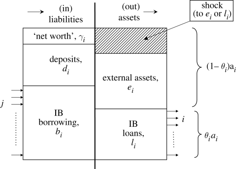
In ecology, the nodes in basic models are simply ‘species’ that are linked to other species/nodes as prey, predator, competitor or mutualist (May 2001; Dunne et al. 2002). In epidemiological networks, the nodes are susceptible, infected/infectious or recovered/immune individuals (Anderson & May 1991; Newman 2002). But in a minimally complicated banking network, the nodes, individual banks, have a more complex structure. Following NYYA and GK, we define such a node/bank as illustrated schematically in figure 1.

Figure 1.

Schematic model for a ‘node’ in the IB network.

Note that, in this deliberately oversimplified scheme, the activities of any given bank are partitioned among four categories. Two of the four categories represent assets: IB lending (l_i) and external assets (e_i). The other two correspond to liabilities: IB borrowing (b_i) and deposits (d_i). Here the subscripts indicate the specific bank, with i = 1, 2, … , N, where N is the total number of banks (table 1). For any individual bank, solvency requires that assets exceed liabilities

2.1

As indicated in figure 1, γ_i is the ‘net worth’ or ‘capital buffer’ of bank i. If e_i, l_i, d_i and/or b_i change in such a way that γ_i becomes negative, then liabilities exceed assets and the bank i is assumed to fail.

Table 1.

The model's key parameters, variables and acronyms.

category	definition	symbol	default value	notes
	number of banks	N	25
balance sheet parameters for individual banks	total assets of each bank	a	1
	IB loans	l	0.2
	lending ratio l/a	θ	0.2
	external assets	e	0.8	e = 1 − θ
	net worth or capital buffer	γ	0.04
IB lending network parameters	average value of loan	w	0.042	w = θ/z
	probability of bank A lending to bank B (Erdos–Renyi probability)	p	0.2
	average number of IB loans (‘mean degree’ of IB network)	Z	4.8	z = p(N − 1)
external asset class parameters	mean number of external asset classes held by each bank, of which c are shared each with g other banks	n (c, g)	5 (5,5)
	for a given asset, fraction of total asset value held by failing banks	x	variable
	simple liquidity shock, caused by discounting assets held by failing banks	LS	α = 2	asset values discounted by a factor e–αx
	more details on liquidity shocks (see text)
	SLS	SLS	α = 2	as above
	WLS	WLS	β = 0.5	discount factor e–βx

In the studies by NYYA, GK and others, these banks are now interconnected in a random, Erdos–Renyi network in which any one of the N banks is linked to any other one, as lender or as borrower (or possibly both), with probability p. In such a network, a bank's average number of incoming/borrowing or outgoing/lending connections, z, will obviously be

2.2

Various assumptions about these parameters can now be made. For a start, more or less by definition, total assets equal total liabilities, as shown in figure 1 (Gai & Kapadia 2007; Nier et al. 2007).

Assumptions about total assets (a_i), net worth (γ_i), IB loans as a fraction of total assets (θ_i) and the average size of any one given bank's individual loans (w_i) can vary. For any given bank, the number of IB loans is equal to the outgoing Erdos–Renyi links (z_i^(out)), and similarly for the number of incoming links (z_i⁽ⁱⁿ⁾). Simulations by different authors make various assumptions about these parameters. Both NYYA and GK assume that γ_i is a fixed fraction of a_i. Both also assume random, Erdos–Renyi networks. NYYA assume that all banks share a common value for the average loan, w. The total value of all assets in the system is fixed, as is the overall system's average value of the ratio of all outgoing loans to all assets, θ. From this, the average value of w, which is assumed to be the value of each and every individual loan, can be calculated as

2.3

Here a represents the value of the total assets of the average bank. Note that z_i^(out) will vary, according to the number of links a given bank has. The calculation of both a_i and e_i(a_i = e_i + z_i^(out)w) is found by a process described in NYYA, and thence θ_i = z_i w/a_i. Thus, θ_i and total assets a_i, and thence net worth γ_i, will vary a bit from bank to bank, depending on z_i^(out).

GK normalize a_i to unity for all banks (whence γ_i is γ, the same for all banks), and they also fix θ_i as a common constant. This implies that w_i varies among banks, proportional to 1/z_i^(out).

Although NYYA briefly explore a model with ‘Big Banks & Small Banks’, most studies we are aware of are confined to simulations assuming a random network.

NYYA's simulations have the default assumptions θ = 0.2, γ = 0.05, N = 25, p = 0.2; their system's total external assets are 10⁵, from which it follows that a = 4000 and w = 167 or w/a = 0.0416. NYYA's simulations show numbers of banks defaulting as shocks progress, allowing individual parameters to vary (specifically γ, p, θ and N each individually varying, while the other parameters are held at the default values). GK make similar choices, fixing θ = 0.2, a = 1, γ = 0.04 and N = 1000 and consider a range of z-values (see equation (2.2)). GK also use a random network, but—as discussed more fully in §5—their assumptions about the propagation of IB shocks differ significantly from those of NYYA.

In the next section, we will compare the results of a simple approximation, which permits analytic and general results, with these numerical simulations. But first it is worth emphasizing some potential extensions in the direction of greater complexity. For one thing, studies of real IB connectivity networks suggest they differ from random in important ways. In particular, the topology of the USA Fedwire system is highly non-random, in a disassociative way: there are a few big banks, each connected to many small banks; small banks are connected to only a few others, mainly large (National Research Council of the National Academies 2007; May et al. 2008). Associated with this is the observation that not only are networks non-random, but there is a very significant distribution in bank sizes. Furthermore, the ratio of net worth/capital buffers to a bank's total assets tends, in fact, to be such that big banks have relatively smaller capital reserves; preliminary studies suggest this is perverse in respect to system stability. We will return to these matters in the concluding section.

3. Initiating and propagating shocks

We follow NYYA, GK and others in studying the consequences of a shock initially hitting any single bank, with the shock taking the form of wiping out a fraction, f, of its external assets. Since we will shortly be resorting to our mean-field approximation, in which all banks have the same values for γ, θ, w and z (with total assets normalized as unity, as in GK, whence e = 1–θ and b = θ), we define this phase I, ‘first phase’, shock as

3.1

This shock term is now to be subtracted from the LHS of equation (2.1), and thus this bank will fail if

3.2

We initially follow NYYA in assuming that this default has no liquidity effects in the disposing of the failing bank's assets, nor on the value of other banks' assets. This implies a loss (s(I)–γ) being distributed equally among the defaulting bank's creditor banks, provided this quantity is smaller than the defaulting bank's total borrowing. If not, then each creditor bank simply loses its total loan (and depositors, external to the IB system, also suffer losses). That is to say the phase I default by a single bank results in each of its z creditor banks experiencing a phase II shock of magnitude

3.3

Here we have, anticipating the mean-field approximation to come, dropped the subscript i that labels the individual failing bank. The notation ‘[a, b]’_MIN in equation (3.3) simply means that we take the lesser of the two quantities a and b.

We will now have a further, phase II, failure of the z banks connected to the initially failing bank if

3.4

This, in turn, may generate phase III failures when these phase II failures of z banks are appropriately distributed among the remaining solvent banks. As outlined below, as a consequence of the possibility of multiple hits arising from the several phase II-failing banks, the criteria for phase III (and subsequent) failures become a bit trickier than equations (3.2) and (3.3) with equation (3.4), even within our mean-field approximation. And so on for phase IV and further.

We emphasize that time does not appear as an explicit variable in the sequence of events, explored below, that may follow as a result of the initial, phase I bank failure. Rather, we simply explore the cascade of successive events that can unfold—dominos falling, as it were—as the initial failure causes phase II failures in banks directly connected by lending or by sharing external assets, in turn possibly causing phase III failures and so on.

Arguably, the most serious deficiency in such a study is that we assume IB borrowing and lending relations remain fixed as this cascade ripples through the system. As emphasized to us by one of three very helpful anonymous referees, a bank threatened with phase II failure as a result of a borrower's default on a loan exceeding γ (i.e. equation (3.4)) could, in principle, simply itself borrow to cover the deficit and thus avoid failing. The problem here, in practice, is that, as the dominos show signs of falling, credit dries up. Indeed, it can be argued that, to quote the referee, recent problems were ‘on the liabilities side of the balance sheet, not the asset side. The Bank of England style models [i.e. GK, NYYA, the present paper] do not capture runs’.

This is a good point. We would argue, however, that in such a scenario the cause of systemic collapse is neither solely on the borrowing side (assets, as in our model) nor solely on the lending side (liabilities), but a combination of both. We nevertheless believe that it is useful to have a clear understanding of the dynamics of possible system collapse, assuming the web of IB borrowing/lending remains static, before proceeding to the much more complicated, although admittedly more realistic, task of elucidating the fully integrated dynamics of such a model system.

4. Shocks propagated by interbank loans

Here we consider the possible knock-on effects of an initial failure, under the rather extreme assumption that the failing bank can dispose of its remaining assets for their original value, and that such sales have no effect on the value of assets held elsewhere in the system. Although clearly artificial, this assumption, following NYYA, sets a baseline for exploration of liquidity effects in subsequent sections.

In addition, as foreshadowed earlier, we begin with a mean-field approximation, replacing the random Erdos–Renyi network by a uniform one in which each bank is connected to exactly z other banks (see equation (2.2)) as a lender and as a borrower. As will be seen, this approximation permits general insights into the way propagation of shocks depends on the system's various parameters, while at the same time agreeing remarkably well with the ensemble average of the numerical simulations by NYYA. Added to the further assumptions that all banks have the same total assets (normalized to unity) and that all loans have the same value, w, we also have that the loan/asset ratio θ is common to all N banks (see equation (2.3)). With all banks thus identically parameterized, the labelling subscripts i can be dropped.

We now proceed to give simple, general formulae for successive phases of failure. The criterion for phase I and phase II failure involves only γ, θ and z. For subsequent phases (III and beyond), we do, however, need to deal with the components of z (p and N), to allow for ‘multiple hits’, once the total number of banks failing in previous phases reaches an appreciable fraction of N. Moreover, in the present approximation scheme, it is easy to retain the parameter f (the fraction of external assets lost in the initiating failure) throughout.

4.1. Phase I failure

Equations (3.1) and (3.2) give this criterion, in terms of f, θ and γ,

4.1

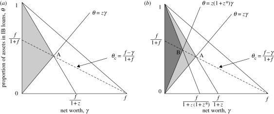
Figure 2a shows the range of values for θ and γ which satisfy equation (4.1), for specified f.

Figure 2.

Regions of IB lending (θ) and net worth (γ) which result in propagation of IB loan shocks. The triangle ‘1, 0, f’ defines the region where loss of a fraction f of a bank's external assets will cause it to fail. In (a), the light-shaded area depicts the region in which creditors of the initially failing bank will receive phase II shocks which cause them also to fail. In (b), the dark-shaded area shows the region in which phase III shocks cause failure.

4.2. Phase II failure

The corresponding criterion for the subsequent failure of each of the z banks which are creditors of the initially failing bank is given by equations (3.3) and (3.4), which can now be written as

4.2

It is helpful now to define θ_c = (f–γ)/(1+f). For θ < θ_c, equation (4.2) reduces to

4.3

Conversely, for θ > θ_c, equation (4.2) becomes

4.4

Again, these simple expressions for the values of γ, θ, z and f which will result in phase II failure of z banks are illustrated (showing γ and θ for specific z and f) by the appropriately shaded region in figure 2a. One particularly interesting result is that under the assumptions of this model no phase II failure is possible if the value of γ—net worth as a fraction of total assets—lies to the right of the point A in figure 2a; this corresponds to the criterion

4.5

4.3. Phase III failure

For phases I and II, the above expressions are exact within the mean-field approximation: when phase I failure occurs, it is transmitted to exactly z banks.

The only relevant parameters are γ, θ, f and z. But for phase III and subsequent failures, we must consider the probable distribution of the z ‘hits’, from each of the z defaulting banks, among the remaining N−(z + 1) = (N–1)(1 − p) banks. There are z² hits in total, but some could fall on the phase I or other (z − 1) phase II failing banks. So, unlike for phases I and II, we need to consider the p and N components of z = p(N − 1).

These complications will arise only if z² represents an appreciable fraction of the total banks. For z² << N, corresponding to p²N << 1, we may simply assume that z² of the previously unaffected banks each experience a single hit. But, more generally, we need to note that each of the (N − 1)(1 − p) unhit banks will experience k = 0,1, 2, … , z hits from the z phase II defaulting banks with probability

4.6

Remember, z is not necessarily an integer, which does not affect formal aspects of our analysis, although in practice it is the simplest to approximate z by the nearest integer. In this more general circumstance, define k_c to be the largest value of k such that (N − 1)(1 − p)p(k_c) is of order unity; that is, the largest k such that one or more previously unhit banks are likely to be hit k times.

In phase III, each of the phase II defaulting banks will, in a manner similar to that discussed for phase II, distribute to each of their z creditor banks a shock of

4.7

The first phase III failures will then occur when one or more banks experience k_c of these shocks, of magnitude such that

4.8

Analysis along that for phase II, mutatis mutandis, now reduces equation (4.8) to the default condition

4.9

and

4.10

Here, for notational convenience, we have defined z* = z/k_c.

As noted above, if N is very much bigger than z², we have k_c ≈ 1 and z* = z. This would be a good approximation if we had N = 250 and p = 0.02, for z = 4.98. NYYA's simulations typically have N = 25 and p = 0.2, for z = 4.8. However, although the z-values are effectively identical (both approx. equal to 5), the phase III behaviour differs. For the (250, 0.02) choice, the probable outcome is that one of the previously unhit 244 banks will suffer two hits, which—depending on equations (4.9) and (4.10) with z* = z/2—may cause the first phase III default; 23 other banks suffer a single hit (z* = z), which may also cause failures depending on the more stringent version of equations (4.9) and (4.10) which ensue. In contrast, for NYYA's (25, 0.2) choice, the average expectation is roughly that one of the 19 previously unhit banks will be hit three times, four will be hit twice, eight once and six not at all.

Thus the ‘k-values’ in equations (4.9) and (4.10) take values of 3 for one bank, 2 for four, 1 for eight, for a total of 13 (of 19) banks potentially affected in phase III; that is, depending on the details, we could see one or five or 13 phase III failures. Figure 2b illustrates the essentials, for the ‘easiest’ (k = k_c) phase III failure.

In analogy to equation (4.5) for phase II, note that phase III failures cannot occur in this model, regardless of the other parameters, if γ exceeds the value indicated by point B in figure 2b and given by equation (4.11) (now interpreting z* = z/k) for each of k = 1, 2, … , z banks hit in phase III

4.11

4.4. Comparison with numerical results

It is interesting to compare these analytic results from the mean-field approximation with NYYA's more exact study in which banks exhibit a statistical scatter in numbers of links (according to the Erdos–Renyi degree distribution). For one thing, in the former case, the phase I → phase II transition, in which the initial failure causes exactly z secondary failures, occurs as a step function at some precise value of the relevant parameters, whereas in the latter (NYYA) case there tends to be a smooth, S-shaped transition. And, of course, the same is true for later transitions, if any. For a given value of a bank's average number of links, z = p(N − 1), note that the fluctuations about this average will be relatively smaller—and the differences between the mean-field approximation and exact simulations therefore also smaller—if this fixed value of z is obtained by larger N values.

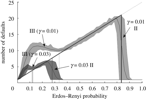
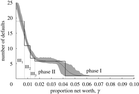
Figures 3 and 4 show that NYYA's exact numerical studies are in reassuring, some might say surprising, agreement with the results obtained from the analytic approximations derived above. The analytic approximation, moreover, helps provide sharper insight into the causes of the observed dynamical behaviour.

Figure 3.

Number of banks failing as a function of percentage net worth (γ). This figure compares the NYYA results with the mean-field approximation (bold line); for further discussion, see the text.

Figure 4.

Number of banks failing as a function of the IB connectivity, p. The figure compares NYYA results with the mean-field approximation (bold line).

Specifically, figure 3 shows numbers of defaults as a function of γ; the other parameters have NYYA's default values (θ = 0.20, N = 25, p = 0.20 (whence z = 4.8) and f = 1). In the mean-field approximation, equation (4.1) then gives the initial single bank failing for γ < 0.80 (!), and equations (4.3) and (4.4) give phase II failure of a further 4.8 banks once γ < 0.042. This agrees with the midpoint of the S-shaped transition at around 0.035–0.048 in NYYA's simulation. For the phase III transition, from equations (4.9) and (4.10), we expect the first failure, of the one thrice-hit bank (k_c ∼ 3; see the discussion above), at around γ = 0.016, with four subsequent phase III failures of twice-hit banks around γ = 0.012 and eight failures of single-hit banks if γ falls below 0.007. In NYYA's simulations, the onset of this phase III progression indeed begins around γ = 0.016. Of course, both the exact simulations and the mean-field approximation predict all banks fail once γ is close to zero.

Figure 4 shows the number of defaults as a function of the link parameter, p, with f, θ and N having their default values, and for two values of γ = 0.01, 0.03. Here the first failure will always occur, and the mean-field approximation, equations (4.3) and (4.4), says there will be a phase II failure of z = 24p banks once p falls below θ/(N − 1)γ : for γ = 0.01 this corresponds to p < 0.83; for γ = 0.03, p < 0.28. Again, these approximate numbers agree well with NYYA's numerical simulations of the full Erdos–Renyi network. Note also that, once p is below the threshold for phase II failure, the total number of banks thus failing is z + 1 = p(N − 1) + 1, whence for γ = 0.01 the linear decline from 21 failed banks at the threshold p = 5/6 toward the initially assumed single bank failure at p = 0. The ‘hump’ that rises against this trend at lower p-values in NYYA's simulations—generating the ‘M-shaped curves’ which they note–of course arises as phase III further failures occur at lower p-values. Again we can estimate these phase III transition points from our equations (4.9) and (4.10), to get the first such failures at roughly p ∼ 0.33 when γ = 0.01, with lower values for larger γ. As p declines towards zero, however, the interlinkage becomes so weak that the number of banks affected by any initial shock clearly must decline to one (i.e. the initially shocked bank itself).

NYYA also give results for simulations of numbers of banks failing as a function of f, θ, and (in three dimensions) of γ and p, in each case with other parameters having their default values. For these further results, the mean-field approximation also gives agreement similar to that seen in figures 3 and 4.

5. Liquidity risk: zero recovery

Up to this point, we have assumed that banks failing had no effect on the assets of other banks, except for the losses suffered by creditor banks. This is unrealistic. There is a significant literature on ‘fire sales’ and their general effect on liquidity; that is, their tendency to depress the value of other institutions' external assets (Pulvino 1998; Cifuentes et al. 2005; Kaufman 2005; Coval & Stafford 2007; Mitchell et al. 2007).

As a first step, it is useful to consider such effects on the disposal of assets of a failed bank, ignoring for the moment the indirect effects elsewhere in the system. This, in effect, is what GK do with their ‘zero recovery’ (henceforth ZR) assumption for shocks otherwise propagating solely by IB loans. In §§3 and 4, we studied what can happen when an initial bank loses a fraction of its external assets which exceed its capital buffer, as given in equation (4.1). The assumption was that the failing bank, and all subsequently failing banks, could dispose of remaining external assets at the ex ante price.

To the contrary, GK assume that once a bank fails (i.e. equation (4.1) applies), then ALL its external assets are lost (hence ZR). This is sensibly justified as a liquidity effect. Although an extreme assumption, it is arguably no less realistic than the opposite extreme of assuming no effects whatsoever.

Be this as it may, the immediate consequence of the ZR assumption is that all creditors of the initially failing bank lose their loans, w_j. In GK's model, with θ and γ fixed, w_j = θ/z_j, where z_j is the number of creditors of the failing bank j. This will, in turn, cause all the z_j creditor banks to fail if, and only if,

5.1

In turn, all these banks will have ZR, with the kth such bank transmitting further shocks of magnitude θ/z_k to each of its z_k creditors and so on. The system's dynamical behaviour in many ways resembles transmission of an infectious disease when an infected individual is introduced into a susceptible population, with the contact network being Erdos–Renyi. GK give a very clear and elegant exposition of this system, with its threshold phenomena and ‘robust yet fragile’ properties.

A mean-field approximation for propagation of shocks under GK's ZR assumption immediately shows there will be no consequences of an initial failure if z > θ/γ. Conversely, for z < θ/γ, the initially failing bank causes all its z creditors to fail, and they in turn will cause failures. In sharp contrast with §4, ZR implies that there is no attenuation of the shock as it progresses through the system. Once N is reasonably large, essentially all the banks in such a ‘uniform’ network will thus fail, once z is below this threshold value. Of course if z is below unity, the system effectively has no interconnections, and for that simple reason there will be no propagation of the initial shock. Thus, the mean-field approximation is again in qualitative agreement with GK's illuminating results. The lower limit on z has a direct parallel with epidemiological studies (the ‘R₀ > 1’ rule; Anderson & May 1991), but the upper limit at around z ∼ θ/γ has no such parallel; it is as if ‘superspreaders’ were rendered uninfectious as a result of their excessive activity.

6. Liquidity shocks: general

A more general approach to liquidity shocks recognizes that the effects of fire sales and liquidity problems are likely to be felt throughout the banking system. There will usually be limits to the capacity of financial markets to absorb an influx of illiquid external assets from a failing bank.

Several studies include the ensuing depression of asset prices by assuming that the value of such illiquid external assets is decreased by a factor (for further discussion, see GK)

6.1

Here x is essentially the number of failed banks as a fraction of the overall total N. The parameter α, in effect, measures the market's sensitivity to such failures: both GK and NYYA put α ≈ 1, corresponding roughly to (GK) ‘the asset price falls by 10 per cent when one-tenth of the system assets have been sold’.

Unlike the earlier studies of the consequences of the initial bank failures, in which shocks are transmitted specifically and only to their z creditor banks, the effects of liquidity risk (modelled in this simplest way) are felt by every bank in the system. That is, if the failure of the first bank in our foregoing system reduces all the other banks' external assets by the factor given in equation (6.1), this amounts to a phase II shock, s*(II), experienced by every one of the remaining N − 1 solvent banks (and distinguished from the phase II shock, s(II) of equation (3.2), which is experienced only by the failing banks' z creditors). We may write

6.2

Here (1 − θ) is the value of the average bank's external assets (with total assets normalized to 1) and β₁ = 1–exp(−αx), with x = 1/N.

From equation (3.3), which now reads s*(II) > γ, we see that this shock could, in principle, cause the entire banking system to crash if

6.3

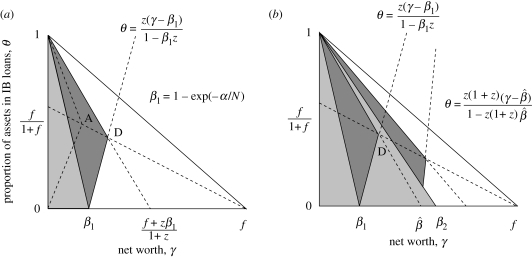
This is illustrated by the shaded area in figure 5a. Notice, from equation (6.3), that all banks may thus fail, provided that θ is small enough, if β₁ > γ.

Figure 5.

(a) This figure, which is to be contrasted with figure 2a, shows the region of θ and γ values within which the initial bank failure causes phase II failures either of all other banks from liquidity shocks (the light-shaded area) or of its z creditors from a combination of liquidity and IB loan shocks (the dark-shaded area). (b) This extends (a), in the same way as figure 2b extends figure 2a, to show phase III failures of the entire system either as a result of liquidity shocks, now amplified by the z phase II failures of (a) (the light-shaded area to the right) or as a result of a combination of this augmented liquidity shock and IB loan shocks from these z phase II failures (the dark-shaded area to the right).

More generally, if γ > β₁, the conditions for the initially failing bank to cause z phase II failures is given by adding the s*(II) of equation (6.2) to the LHS of inequality equation (3.4). The appropriate extension of equation (4.2), including the effects of liquidity risk, then leads to the criterion for phase II failure of z banks

6.4

With θ_c as previously defined (just below equation (4.2)), equation (6.4) gives the criteria for phase II failure of z banks as

6.5

and

6.6

This is illustrated by the dark-shaded area in figure 5a.

As in figure 2 and equation (4.5), there is a γ value above which phase II failures cannot occur. This is indicated by point D in figure 5a. The explicit criterion, expressed in terms of β₁, f and z, is

6.7

Figure 5a also illustrates the obvious fact that phase II failures are easier once the effects of liquidity risk are taken into account, as they usually should be (in figure 5a, point A is as in figure 2, corresponding to D in the absence of liquidity risk, α = 0).

For completeness, we now set out the corresponding criteria for phase III failure. Here each of the (N − 1)(1 − p) remaining banks experiences a liquidity risk shock of magnitude

6.8

Here β₂ = 1–exp(−αx₂), with x₂ = (1 + z)/N. The criterion corresponding to equation (6.2) for total failure of the system, following the phase II failure of the initially failing bank's creditors, is thus

6.9

This cannot happen if γ > β₂, but otherwise can if θ is sufficiently small (figure 5b).

Phase III failures among the creditors of the z phase II failing banks can be estimated along the lines which earlier gave us equations (4.9) and (4.10). Adding the appropriate term β₂(1 − θ) to the s(III) shock of equation (4.7), we get the criteria for phase III failure, including liquidity risk, as

6.10

and

6.11

Here β₁ and β₂ are as defined above, and z* = z/k is as discussed in deriving equations (4.19) and (4.10). This is illustrated in figure 5b. Note how liquidity shocks, once they get going, can bring the whole system down, even for γ values that would effectively protect the system against IB loan shocks (compare figures 2 and 5).

So long as the total number of failed banks is significantly less than N, the above analyses can be extended to phase IV and subsequent failures (in a routine but tedious way).

7. Strong and weak liquidity shocks

The previous two sections have introduced liquidity risk in a rather broad-brush fashion. We now present some new ideas, which take account of liquidity risks in a way which—while still no more than crude caricature—take some steps in the direction of greater realism.

Suppose each of our N banks has its external assets (e_i = [1 − θ_i] a_i or e = [1 − θ] under our usual assumption that all banks are of the same size, normalized to unity, and that all have the same value of θ) made up of n distinct ‘asset classes’, each of equal value (namely [1 − θ]/n). Suppose further that c of these n are shared (n ≥ c ≥ 0), each among a total of g other banks (N ≥ g ≥ 1). Note, incidentally, that this implies the total number of distinct asset classes is N[n − c(g − 1)/g]: in the limit when all banks share all assets, n = c and g = N, then we have a total of n distinct classes; in the opposite limit when none are shared, the total is Nn.

We now adopt a somewhat more detailed approach to accounting for discounting assets or liquidity risks. Following earlier studies (NYYA, GK, etc.), we start things off with the artificially extreme assumption that the initial bank failure is caused by one asset of one bank having its value go to zero (i.e. f = 1/n). More realistically, all that is required is that the value of this asset decreases by an amount in excess of the capital buffer, γ; our extreme assumption has the virtue of keeping things simple, without significant loss of generality. We now discount all assets in that specific class held by other banks by a factor exp(−α/g). This corresponds to the earlier equation (6.2), and represents an SLS, of magnitude

7.1

As such SLS propagate, causing or contributing to the failure of other banks; the strong shock to this asset class becomes more severe, corresponding to a discount factor exp(−αk/g), where k represents the total number of failed banks holding such assets.

So much for liquidity problems resulting from the particular asset class that precipitates events by causing the initial bank failure. But what of other asset classes held by this initial bank? These are likely also to experience depreciation, as a result of the initially failing bank's ‘fire sale’ and/or a non-specific (emotional?) loss of market confidence in such other assets held by a failed bank.

We believe that it is useful to explore the dynamical behaviour of banking systems in which a distinction is drawn between liquidity shocks caused by the explicit failure of a specific asset class, and the more general ‘loss of confidence/trust’ that this can provoke throughout the system. To this end, we define WLS as resulting from the discounting of all other asset classes held by the initially failing bank. Following this initial bank failure, the relevant discount factor is exp(−β/g), experienced by each of the (g − 1) banks which share any one of this bank's asset classes.

In later phases, a single bank could suffer multiple hits from k failing banks, each holding a particular previously unhit asset class, in which case the WLS discount factor is exp(−βk/g).

We now explore a range of assumptions about the relative severity of SLS and WLS, as characterized by the relative value of the discount parameters α and β (α ≥ β ≥ 0).

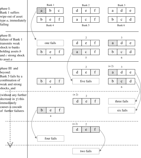
When SLS, WLS and IB shocks, singularly or in combination, cause further bank failures, we additionally assume that any weakly shocked asset class held by any such subsequently failing bank is transformed into a SLS to that asset class as held by other banks still in the system. Figure 6 hopes to illustrate this SLS/WLS scheme. Such a scheme, where both SLS and WLS grow as more banks fail, serves as a crude half-way house between a general equilibrium asset-pricing model (itself not free from problems) and the simple approach outlined in §6 (which is arguably too simple).

Figure 6.

Schematic illustration of SLS and WLS, for a system of N = 6 banks, each holding n = 3 asset classes, each of which is shared (c = n) among g = 3 banks. Initially, Bank 1 experiences total loss of its asset a. If this asset's value exceeds the capital buffer γ, phase I failure of this bank ensues; there follow SLS to a assets held by other banks, and WLS to b and c assets. Phase II failure, caused by liquidity effects, follows for the most strongly affected Bank 5, if γ further decreases such that the value of one SLS plus one WLS exceeds γ. There are consequent liquidity effects on the remaining four banks. In this example, we see a cascade of further failures as—without any additional decrease in γ needed—Banks 3 and 6 fail, causing Bank 4 to fail, and thence the remaining Bank 2. Squared box, initial asset wipe-out; dotted box, asset class receiving weak shock; hatched box, asset class receiving strong shock.

We now present and discuss a series of numerical simulations—all of whose main features can be understood (in some numerical detail) by the mean-field approximation—illustrating the effects of such combinations of SLS and WLS along with IB loan shocks.

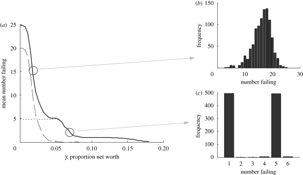
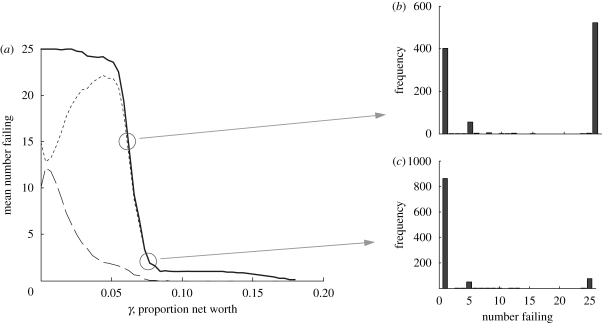
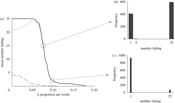
Figures 7–9 show the number of failures in a 25-bank system as a function of the capital reserve, γ. The other parameters have the usual default values: a = 1, θ = 0.2, p = 0.2 (whence z = 4.8). In these simulations, each bank's external assets are divided equally among five asset classes, each of which is shared among five banks (i.e. n = c = g = 5). Initially, a single bank loses the entire value of one asset class (s(I) = 0.16), and if this bank consequently fails, this particular asset class, which is held by four other banks, will experience an SLS with discount parameter α = 2 (see equation (6.1)). The initially failing bank will also propagate WLS to four other banks holding each one of its four other asset classes (for a total of 16 WLS, some of which are likely to be multiple hits on other banks). These WLS are characterized by discount parameters β = 0, 0.01, 0.5 for figures 7–9, respectively.

Figure 7.

Average number of banks failing, over 10³ simulations and as a function of γ in a simulation with IB links and SLS. n = c = g = 5, with no WLS. In (a), the long-dashed curve shows mean number of banks suffering mainly IB shocks at the point of failure. The short-dashed curve shows mean number of banks failing mainly from liquidity shocks. Solid line, all; α = 2, β = 0. (b,c) Frequency distributions for numbers of banks failing for two different values of γ ((b) γ = 0.017 and (c) γ = 0.064). For more full discussion of this and subsequent figures, see the text.

Figure 8.

As in figure 7, but with very WLS, β = 0.01 (a). (b) γ = 0.062 and (c) γ = 0.074. Solid line, all; long-dashed line, mainly IB; short-dashed line, mainly Liq.

Figure 9.

As in figure 7, but with WLS, β = 0.5 (a). (b) γ = 0.076 and (c) γ = 0.096. Solid line, all; long-dashed line, mainly IB; short-dashed line, mainly Liq.

In figure 7, β = 0 and so there are no WLS. The solid curve shows the number of banks failing as an average over 10³ simulations, assuming the banks to be connected by a random, Erdos–Renyi network of IB lending along with shared asset classes, as defined above. We do not show the statistical spread of the simulations, as done earlier in figures 3 and 4, because the present figures are arguably cluttered enough!

Considerable insight into figure 7, and the subsequent ones, is provided by the mean-field approximation, as follows. The initial shock has magnitude s(I) = 0.16; hence, the initial failure occurs once γ < 0.16. From equation (6.1) with α = 2, this will propagate an SLS of magnitude 0.053 to the four other banks that share this particular asset class. In addition, the initial failure will, from equation (3.3), result in a phase II shock of magnitude s(II) = (0.16 − γ)/z to the bank's z creditors; with z = 4.8 in this mean-field approximation, this becomes s(II) = (0.033 − γ/4.8). The distribution of these two different shocks among the initially remaining 24 banks is such that the probability of one of the four banks experiencing the SLS also receiving an IB loan shock is roughly unity; such a bank will fail if 0.053 + (0.033 − γ/4.8) > γ or γ < 0.071. Allowing for the ‘statistical smudging’ introduced by the fact that the simulated network is random, not uniform, these observations are explained in figure 7: after the initial failure, the overall probability of phase II failure arising does indeed begin around γ = 0.07 and saturates to all four SLS banks having failed at around γ = 0.05. Furthermore, once any one of the four banks experiencing SLS fails, the discount factor of equation (6.1) strengthens to exp(−2α/5), resulting in SLS of 0.088 to the remaining three, which immediately fail. Figure 7c illustrates this: in the range 0.07 ≥ γ ≥ 0.05, any one γ value corresponds to simulations in which either only the first bank has failed or else all five have, in proportions that increase as γ decreases.

Beyond the first five failures in this figure, there are no more liquidity shocks. Subsequent failures occur as γ decreases, caused by IB loans propagating shocks (which are attenuated in each subsequent phase), as discussed earlier and illustrated in figure 2. Figure 7b shows that there is, as would be expected, a more Gaussian distribution of failures resulting from statistical scatter in this region, as the system's average behaviour moves to failure of all banks as γ → 0. Finally, note that the dashed curves in figure 7 support the discussion above, indicating roughly the proportional contributions of SLS and IB shocks to the number of failures, as a function of γ.

Figure 8 gives the corresponding results for the case where all parameters are the same, except that there are now very WLS, with the discount factor being β = 0.01 (in contrast with the SLS α = 2). The system's behaviour is, however, radically different. This results from our assumption that unaffected assets of a failing bank transmit only WLS, but if a bank possessing one (or more) weakly shocked assets fails, then other banks sharing this asset (or assets) experience such failure as an SLS. Going back to figure 7, we recall that the initial failure will begin to cause phase II failures, resulting from a combination of SLS and IB shocks, at around γ ∼ 0.07. But once a single such phase II failure occurs, the chance of that bank also receiving a WLS from one of the other four assets owned by the initially failing bank is 1 − (1 – 4/24)⁴ = 0.48. So there is a roughly 50 per cent chance that the initial phase II failure will not only strengthen the original SLS, but more significantly will propagate new SLS to the three other banks sharing its WLS. And so on. Even for the tiniest value of the WLS parameter β, a cascade of SLS failures is likely to ensue in the fairly tightly interlinked (n = c = g = 5) system under study. This is seen in figure 8, where the dashed curves indicate that, until γ is small, most of the failures are caused by liquidity shocks, not unlike the simplistic treatment of liquidity shocks in §6. Figure 8b,c amplify this: as the cascade of failures begins (figure 8c), very few simulations have any failure other than the initiating one, but the few simulations that do show failures bring the entire system down, and thus have disproportionate effects on the average number of failures; quite small further decreases in γ result in a much higher proportion of all banks having failed (figure 8b).

Figure 9 shows what happens when β has more substantial values. Not only do we have the cascades of figure 8 induced as WLS are transformed into SLS, but the WLS are themselves of significant magnitude: [1 − exp(−β/5)] (0.16) = 0.015 for β = 0.5. Along the lines indicated above, we can estimate that the probability of any one of the four banks receiving an SLS from the initial failure also receiving from it a WLS and an IB loan shock is around 10 per cent, corresponding roughly to an overall 40 per cent chance of such an event. Such a triple shock will cause failure once γ > 0.084. This explains the earlier onset of the cascade in figure 9.

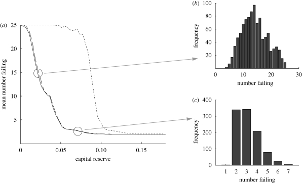
In contrast with figures 7–9, figure 10 summarizes parallel results for n = c = g = 2, α = 2 and β = 0, 0.01, 0.5. The external assets of the banks in this system are substantially less interlinked, although the magnitude of any one asset class held by a bank is corresponding larger. Here s(I) = 0.40, corresponding to the initial bank failing for γ < 0.40. The SLS from this failure affects only one other bank, producing s(II) = 0.252, and failure for γ < 0.252. So the first two failures have occurred for γ off the scale in figure 10. Given the low degree of interactivity in this system, for a tiny value of β (0 or 0.01), subsequent failures will be caused by IB shocks. These will first arise if any one of the other 23 banks incurs an IB shock from both failing banks. A somewhat more complicated mean-field calculation than those above shows that this first happens at γ = 0.078; the probability of such a double hit is 4 per cent for any one bank, amounting to an expectation of one such bank failure at this γ value. Failures caused by single IB hits abound once γ < 0.042, and the curve rises—with essentially no difference between β = 0 and 0.01—to total system failure at very low γ values. Conversely, for appreciable values of β, the next failure after the first two is likely to arise from a combination of an IB shock (from the initially failing bank) and a WLS (of magnitude 0.088 from either bank) below γ = 0.130; this event has average probability roughly 61 per cent. Below this γ value, the curve climbs steeply. Again, this mean-field calculation agrees with the simulations shown in figure 10.

Figure 10.

As in figure 7, but with less interlinkage of assets among banks: n = c = g = 2. Mean numbers failing are shown for (a) β = 0 (solid line), 0.01 (long-dashed line) and 0.5 (short-dashed line). (b) γ = 0.022 and (c) γ = 0.059.

The contrast between figures 7–9, where interactions through shared asset classes are relatively strong, and the corresponding figure 10, where they are not, should be noted. The differences show up both in the main figures (part (a)) for failures versus γ and, perhaps more interestingly, in the insets to the right margin (parts (b) and (c)) which further illuminate the simulation results.

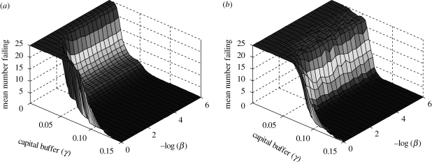
As emphasized above for systems with a substantial degree of interlinkage via shared asset classes, the major effects exerted by WLS with tiny discount factors (very small β) derive from the assumption that such WLS are propagated as SLS when a bank holding them fails. Figure 11 contrasts this assumption about accelerating discounting of assets held by failing banks with the opposite extreme of having a failing bank's WLS transmitted unchanged to other banks holding this asset, as unaugmented WLS. In figure 11a, where WLS → WLS, such shocks are essentially irrelevant once the characteristic discount parameter β is less than 0.01 or so. In figure 11b, where WLS → SLS, we find catastrophic collapse for arbitrarily small β, unless of course β is strictly zero (corresponding to no WLS at all).

Figure 11.

Mean number of banks failing as a function of γ and the WLS parameter β. (a) The case where WLS remain weak throughout successive bank collapses. This contrasts with figures 7–10, where WLS become ‘strong’ where they cause bank collapse (z = 4.8, WLS → WLS). (b) The case where WLS become ‘strong’ where they cause a bank collapse (z = 4.8, WLS → SLS). This is the same process as in figures 7–10.

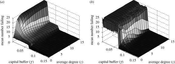
The ‘three-dimensional’ figure 12a,b extend figures 7 and 8, respectively, to show numbers of failing banks in terms of both β and z, the average number of links between nodes in the Erdos–Renyi network (z = p [N − 1]). While the onset of precipitous collapse occurs later when β = 0 than for β = 0.01, the basic features for arbitrary z-values are similar to those seen for the particular value z = 4.8 in figures 7 and 8. That is, the ‘degree distribution’ or connectivity of the IB loan network has relatively little effect on the dynamics of the system here. This, in turn, is a consequence of the fact—implicit in the assumption about SLS and WLS, along with the parametrization of the models—that shocks here are propagated in an unattenuated, even amplified, way by liquidity effects.

Figure 12.

Mean number of banks failing as a function of the capital buffer and the mean number of IB connections. Here N = 25, n = c = g = 5, α = 2 and (a) β = 0, (b) β = 0.01.

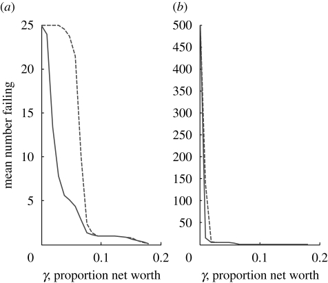
Last but not least, figure 13 contrasts numbers of failing banks as a function of γ for the parameter values used in figures 7 and 8 (a = 1, θ = 0.2, n = c = g = 5, α = 2, β = 0 or 0.01, p = 0.2 and N = 25, i.e. z = 4.8) with the system's dynamics for the same parameter values except that N = 500 and p = 0.02, so that z = 10. The latter system is clearly less interwoven than the former; although the average bank has more connections (10 versus 4.8), as a proportion of all possible connections they are much smaller (2 versus 20%). Clearly, the less interlinked system is more robust.

Figure 13.

A comparison of mean numbers of banks failing (a) for a ‘highly concentrated’ system (25 banks) and (b) for a less concentrated system (500 banks). In the former case, z = 4.8, and in the latter, z = 10. Solid line, β = 0; dashed line β = 0.01.

8. Discussion

As emphasized at the beginning, the model studied in this paper as a mathematical metaphor for financial, particularly banking, networks is a deliberate and extreme oversimplification. Its essential assumptions are, however, based on earlier work, which has arguably produced interesting and potentially important insights.

Before proceeding to sketch ‘lessons learned’, we re-emphasize a couple of new and distinctive elements in the present work. One is the use of mean-field approximations to give general analytic insight into the dynamical behaviour of randomly connected networks of banks. The approximations are consistently compared with the corresponding results from numerical simulations by others and by ourselves (for particular parameter values), and they agree well, perhaps surprisingly well. Another is the introduction of a distinction between SLS and WLS to banks’ external assets, following bank failures elsewhere in the system.

More generally, we study models that are a network of networks. In some ways, the simplest, and the most amenable to comparison with real banking systems, is the explicit network of IB borrowing and lending. There are, however, also many less directly evident interconnections among banks, deriving from particular subsets of banks sharing external assets of different kinds. In our oversimplified terms, these can be thought of as a multitude of separate networks, pertaining to different categories of variously shared classes of external assets.

When a bank fails, the consequences for creditors whose loans cannot be paid are direct. The effects of loss of a particular asset class by a particular bank—often treated by some overall average ‘liquidity loss’—is trickier, ranging from specific failure of some class of such assets (e.g. subprime mortgages) through reappraisal of the tendentious worth of some asset class whose original value was assigned carelessly or incompetently (e.g. bundles of credit default swaps) (Bolton et al. 2009) to the intangible psychological effects of ‘loss of confidence’. We have introduced the notion of SLS and WLS with the hope of capturing some of the complexity of liquidity shocks, while at the same time recognizing that this is only a beginning (one step beyond the conventional equation (6.1)).

Given that our models are at best metaphors, and not intended as 1 : 1 maps of reality, it did not seem sensible to complicate things unduly. We cannot, however, resist noting some extensions to the present work which could be useful.

Our model system consists of N banks, all of the same size, and with interconnections at random (specifically Erdos–Renyi networks of given degree, or approximated as uniform). It is clear that real banking systems are far from randomly connected, typically being ‘longtailed’, and with banks varying greatly in size (e.g. National Research Council of the National Academies 2007). Moreover, within these long-tailed networks, the connections are not ‘proportional’, but often seem more typically to be ‘disassortative’: relatively few big banks are superspreaders, connected predominantly to small banks, while the more numerous small banks are connected predominantly to big ones (National Research Council of the National Academies 2007). Recent work on real ecosystems and their dynamical behaviour suggests that such overdispersed and disassortative systems tend to be more resistant to certain kinds of perturbation (Bascompte et al. 2006; May 2006; May et al. 2008; Sugihara & Ye 2009). Conversely, epidemiological studies suggest disassortative networks are more effective in spreading infection than are assortative ones (which tend to spread faster but ‘burn out’) or proportionately mixed ones (Gupta et al. 1989). In short, we need to know more both about interconnections among real banks and about the properties of non-random interactions among big banks and little banks.

It would also be useful to extend our distinction between SLS and WLS, with their characteristic discount parameters α and β, to a more nuanced distribution of categories of liquidity shocks, described by some distribution {α_i} of α values.

Despite its artificial simplicity, the present paper does tend to support some thoughts circulating about ‘what needs to be done’, as follows.

First, note that shocks propagated by defaults on IB loans tend to attenuate, by a factor of order z, in each successive phase. For example, if each bank is on average connected to five other banks in a many-bank system (N ≫ 1), by phase IV the initial shock tends to be attenuated by roughly two orders of magnitude (1/5³ = 1/125); for smaller N, multiple hits can complicate things, weakening such attenuation factors. Furthermore, high degrees of concentration or connectivity, which are a worry with respect to spreading ill-effects (resulting in R₀ ≫ 1 for infectious diseases), mean that such IB loan shocks are attenuated correspondingly rapidly (it is almost as if superspreaders become less infectious by virtue of their high activity level). By contrast, liquidity shocks—both strong and weak in our scheme—do not experience attenuation; to the contrary, for a given asset class, they tend to grow as more and more banks hold the failing asset (see figure 5b or recall the amplification from exp(−α/g) to exp(−αk/g) following equation (6.1), where k is the number of failing banks). Among other things, this emphasizes, not that it should be needed, the importance of placing a careful and accurate value upon an asset class in the first place. Failure to do so can create rapidly expanding liquidity shocks.

Second, figures 2 and 5 and the accompanying equations and text make it plain that the zone of instability with respect to IB loan shocks is maximized by having θ not too big or small, corresponding to a rough balance of IB loans and external assets. In some ways, this relates to the disadvantage of homogeneity within the system, as discussed below. In a very rough sense, intermediate values of θ correspond to substantial blending of investment banking and retail banking; Glass–Steagall was perhaps good for system stability.

Third, it is trivially obvious that having large buffers, γ, will make for greater robustness both of individual banks and of the system as a whole. But there is the corresponding non-trivial cost of potential working capital lying idle. Both naive intuition and empirical evidence suggest that banks tend to move γ to lower levels in boom times, when things seem good and opportunities abound. To the contrary, the UK Financial Services Authority (Strachan 2009) and HSBC's Stephen Green (Financial Times 2009) have suggested that boom times provoke riskier behaviour and bust times conservatism, which suggests that γ should be relatively larger in the former times (and relatively lower in the latter, to free up capital for sound loans). But you do not need mathematical models to see this! Less transparent is the question of whether all banks should—from a systematic risk perspective—have the same ratio of capital reserves, γ, to total assets, a, or whether big banks should have larger, or alternatively smaller, such ratios than small banks. The present paper is silent on this issue, having confined attention to same-size banks. Preliminary work, however, tends tentatively to support the case for big banks holding relatively higher capital reserve ratios than small banks (which is contrary to existing trends; Haldane 2009).

Fourth, there is a question about the relationship between systemic risk and homogeneity within the banking system. N. Beale & D. Rand (2009, personal communication) and N. Beale et al. (2009, personal communication) have brought this issue into sharp focus with a model whose essence can be illustrated as follows. Suppose we have N banks, and in the notation of §7 also have n = N distinct asset classes. Suppose further that each asset class has some very small probability, ϵ, of having its value decline to the extent that a bank holding solely that asset would fail; these asset classes are furthermore completely uncorrelated. In situation A, each of the N banks holds one asset class, in its entirety. Clearly, the probability for any one bank to fail is ϵ, while the probability for the whole system to fail is ϵ^N. In situation B, every individual bank holds a fraction 1/N of every one of the N asset classes; all banks are identical. It is easy to show that, for sufficiently small ϵ (specifically, ϵ < 1/N), the probability for any one bank to fail is now (ϵ N)^N/N!, which for large N is approximately (ϵe)^N(2πN)^−½, with e = 2.718. For small ϵ, this quantity is much smaller than ϵ (essentially as a consequence of the central limit theorem, from averaging over the N different asset-class risks). But all banks are identical in situation B, which implies this expression—which is of the general order of ϵ^Ne^N—is much bigger than ϵ^N. In short, in this illustrative example of Beale and Rand's more general analysis, situation A puts each individual bank at much greater risk than situation B, but conversely the entire banking system is at much greater risk in situation B than in situation A. The interest of individual banks is to move to the homogenizing limit of B (and arguably the Basel Accords prompted and/or facilitated this), but systemic risk is thereby greatly increased, to the detriment of the wider community. We have, in effect, what evolutionary biologists would call the Prisoner's Dilemma or ecologists the Tragedy of the Commons.

Our discussion of WLS and SLS, under various assumptions about the degree to which asset classes are shared among banks, can be seen as illustrating this general message, albeit in a modest way. Figures 7–9 represent a banking system with comparatively greater homogeneity (n = c = g = 5; all banks hold five asset classes, all shared, each with four other banks) than that of figure 10 (n = c = g = 2; all banks hold two asset classes, both shared, each with one other bank). For WLS with small β, the relatively less homogeneous system of figure 10 can be seen to collapse at lower γ values than the relatively more homogeneous system of figure 8; that is, the former is less fragile than the latter. This is true despite the fact that the shock which causes the initiating bank failure is bigger in figure 10 than in figure 8 (s(I) = 0.40 for figure 10, 0.16 for figure 8). In figure 3, asset liquidity effects are omitted. In effect, this represents the limiting case where banks are totally inhomogeneous (akin to situation A above), with shocks propagated solely by defaults on IB loans. The domain of systemic collapse in figure 3 is smaller than that shown in any of the effectively less inhomogeneous systems illustrated in figures 7–12 (although in particular limiting circumstances they can coincide). As acknowledged earlier, our treatment of liquidity shocks was partly prompted by Beale and Rand's work, which we sought to embed in a more conventional framework. Be this as it may, §7 does illustrate the destabilizing effects of homogeneity upon the systems as a whole, although not as clearly as the ‘thought experiment’ in the previous paragraph. In conclusion, this fourth message is an important one.

References

- Anderson R. M., May R. M. 1991. Infectious diseases of humans: dynamics and control. Oxford University Press. [Google Scholar]
- Bascompte J., Jordano P., Olesen J. M. 2006. Asymmetric coevolutionary networks facilitate biodiversity maintenance. Science 312, 431–433. ( 10.1126/science.1123412) [DOI] [PubMed] [Google Scholar]
- Battison S., Delli Gatti D., Gallegati M., Greenwald B., Stiglitz J. E. 2009. Liaisons dangereuses: increasing connectivity, risk sharing, and systemic risk. Working Paper.
- Bernanke B. S. 1983. Nonmonetary effects of the financial crisis in the propagation of the Great Depression. Am. Econ. Rev. 73, 257–276. [Google Scholar]
- Bolton P., Freixas X., Shapiro J. 2009. The credit ratings game. NBER Working Paper 14712. See http://www.nber.org/papers/w14712.pdf.
- Cifuentes R., Shin H. S., Ferrucci G. 2005. Liquidity risk and contagion. J. Eur. Econ. Assoc. 3, 556–566. [Google Scholar]
- Coval J., Stafford E. 2007. Asset fire sales (and purchases) in equity markets. J. Financ. Econ. 86, 479–512. ( 10.1016/j.jfineco.2006.09.007) [DOI] [Google Scholar]
- Dunne J. A., Williams R. J., Martinez N. D. 2002. Food-web structure and network theory: the role of connectance and size. Proc. Natl Acad. Sci. USA 99, 12917–12922. ( 10.1073/pnas.192407699) [DOI] [PMC free article] [PubMed] [Google Scholar]
- Elton C. S. 1955. The ecology of invasions by animals and plants. London, UK: Methuen. [Google Scholar]
- Financial Times 2009. HSBC chief echoes call to review ratios. See http://www.ft.com/cms/s/0/a015ccdc-196b-11de-9d34-0000779fd2ac.html?ftcamp=rss&nclick_check=1.
- Gai P., Kapadia S. 2007. Contagion in financial networks. Mimeo, Bank of England. See http://www.csef.it/Unicredit_conference/Gai_Kapadia.pdf.
- Gardner M. R., Ashby W. R. 1970. Connectance of large dynamic (cybernetic) systems: critical values for stability. Nature 228, 784 ( 10.1038/228784a0) [DOI] [PubMed] [Google Scholar]
- Goldenfeld N., Kadanoff L. P. 1999. Simple lessons from complexity. Science 284, 87–89. ( 10.1126/science.284.5411.87) [DOI] [PubMed] [Google Scholar]
- Gupta S., Anderson R. M., May R. M. 1989. Networks of sexual contacts: implications for the pattern of spread of HIV. AIDS 3, 807–817. [PubMed] [Google Scholar]
- Haldane A. G. 2009. Rethinking the financial network. See http://www.bankofengland.co.uk/publications/speeches/2009/speech386.pdf.
- Hutchinson G. E. 1959. Homage to Santa Rosalia; or, why are there so many kinds of animals. Am. Nat. 93, 145–159. [Google Scholar]
- Kaufman G. G. 2005. Bank contagion: a review of the theory and evidence. J. Financ. Serv. Res. 8, 123–150. ( 10.1007/BF01053812) [DOI] [Google Scholar]
- MacArthur R. H. 1955. Fluctuations of animal populations and a measure of community stability. Ecology 36, 533–536. ( 10.2307/1929601) [DOI] [Google Scholar]
- May R. M. 1972. Will a large complex system be stable? Nature 238, 413–414. ( 10.1038/238413a0) [DOI] [PubMed] [Google Scholar]
- May R. M. 2001. Stability and complexity in model ecosystems. Landmarks in Biology. 1973 (re-issued, with retrospective Introduction) Princeton University Press. [Google Scholar]
- May R. M. 2006. Network structure and the biology of populations. Trends Ecol. Evol. 21, 394–399. [DOI] [PubMed] [Google Scholar]
- May R. M., Levin S. A., Sugihara G. 2008. Complex systems: ecology for bankers. Nature 451, 893–895. ( 10.1038/451893a) [DOI] [PubMed] [Google Scholar]
- Mitchell M., Pederson L. H., Pulvino T. C. 2007. Slow moving capital. AEA Pap. Proc. 97, 215–200. [Google Scholar]
- National Research Council of the National Academies 2007. New directions for understanding systemic risk: a report on a Conference Cosponsored by the Federal Reserve Bank of New York and the National Academy of Sciences. Washington, DC: The National Academies. [Google Scholar]
- Newman M. E. J. 2002. Spread of epidemic disease on networks. Phys. Rev. E Stat. Nonlinear Soft Matter Phys. 66, 016128. [DOI] [PubMed] [Google Scholar]
- Nier E., Yang J., Yorulmazer T., Alentorn A. 2007Network models and financial stability. J. Econ. Dyn. Control 31, 2033–2060. ( 10.1016/j.jedc.2007.01.014) [DOI] [Google Scholar]
- Oltvai Z. N., Barabasi A. L. 2002. Life's complexity pyramid. Science 298, 763–764. ( 10.1126/science.1078563) [DOI] [PubMed] [Google Scholar]
- Pulvino T. C. 1998. Do asset fire sales exist? An empirical investigation of commercial aircraft transactions. J. Finance 53 ( 10.1111/0022-1082.00040) [DOI] [Google Scholar]
- Strachan D. 2009. The regulatory response of the G20 to the financial crisis. See http://www.fsa.gov.uk/pages/Library/Communication/Speeches/2009/0401_ds.shtml.
- Sugihara G., Ye H. 2009. Co-operative network dynamics. Nature 458, 979–980. ( 10.1038/458979a) [DOI] [PubMed] [Google Scholar]
- Various Authors 2009. Special section on complex systems and networks. Science 325, 405–432. ( 10.1126/science.325_405) [DOI] [PubMed] [Google Scholar]