Transient virulence of emerging pathogens

Abstract

Should emerging pathogens be unusually virulent? If so, why? Existing theories of virulence evolution based on a tradeoff between high transmission rates and long infectious periods imply that epidemic growth conditions will select for higher virulence, possibly leading to a transient peak in virulence near the beginning of an epidemic. This transient selection could lead to high virulence in emerging pathogens. Using a simple model of the epidemiological and evolutionary dynamics of emerging pathogens, along with rough estimates of parameters for pathogens such as severe acute respiratory syndrome, West Nile virus and myxomatosis, we estimated the potential magnitude and timing of such transient virulence peaks. Pathogens that are moderately evolvable, highly transmissible, and highly virulent at equilibrium could briefly double their virulence during an epidemic; thus, epidemic-phase selection could contribute significantly to the virulence of emerging pathogens. In order to further assess the potential significance of this mechanism, we bring together data from the literature for the shapes of tradeoff curves for several pathogens (myxomatosis, HIV, and a parasite of Daphnia) and the level of genetic variation for virulence for one (myxomatosis). We discuss the need for better data on tradeoff curves and genetic variance in order to evaluate the plausibility of various scenarios of virulence evolution.

1. Introduction

Are emerging pathogens unusually virulent? While news reports of emerging pathogens such as avian influenza, severe acute respiratory syndrome (SARS) or West Nile virus (WNV) often suggest that their virulence is related to their novelty, there is only weak theoretical support for the idea that novel pathogens should be unusually virulent. Under what circumstances will emerging pathogen strains be more virulent than their ancestors?

Epidemiologists once believed that pathogens would inevitably evolve towards mutualism, but in the last two decades this group-selectionist ‘classical dogma’ (Levin & Svanborg-Eden 1990) has given way to a richer view of virulence dynamics (Levin & Pimentel 1981; Frank 1996; Ebert 1999; Dieckmann et al. 2002; Ebert & Bull 2003). This body of theory, however, gives few compelling reasons that emerging pathogens should be biased towards high virulence.

One pattern sometimes observed in emerging pathogens is high virulence when the pathogen is first observed, followed by a rapid decrease in virulence, sometimes within a small number of host generations (Dwyer et al. 1990; Knell 2004). A lack of evolved resistance or tolerance in novel hosts could explain the initially high virulence of emerging pathogens: in addition to the obvious direct effects of low tolerance or resistance on host death rate or case mortality, we can also predict that pathogens adapted to resistant hosts would express higher levels of virulence in non-resistant hosts (Mackinnon & Read 2004). While pathogens might adapt quickly to their new host environment, host evolution alone would have difficulty explaining post-emergence decreases in virulence within a small number of host generations.

Other mechanisms driving observed high initial virulence in emerging pathogens include sampling bias (i.e. the fact that emerging pathogens are more likely to be detected if they are highly virulent); a high level of co-infection (and hence within-host competition, driving selection for higher virulence) in diseases with high prevalence; poor host nutritional status (Beck et al. 2004); and, in human ‘virgin-soil’ epidemics, the breakdown of societal support systems (Johnston 1987). Explanations for decreasing virulence are scarcer. If the initial high level of virulence is maladaptive (e.g. because the parasite is an introduced or escaped biocontrol agent that has been selected for hypervirulence, or because of drift or mutation in the transition to the novel population), then selection will drive it down; if epidemics drive down host population densities, then the changing ecological setting can select for lower virulence (Lenski & May 1994).

Could eco-evolutionary dynamics, as well as changes in the host genetic background, drive initially high virulence and rapid subsequent decreases in virulence in emerging pathogens? Current theories of virulence attempt to predict the evolutionary optimum virulence, defined as the rate of pathogen-induced host mortality, for a pathogen whose prevalence is stable over time. If transmission rate increases with increasing virulence (e.g. as a result of increased within-host replication), but the transmission benefits associated with increased virulence decelerate at high levels of virulence, then pathogen virulence will approach a stable evolutionary equilibrium. As Frank (1996), Day & Proulx (2004), and Bull & Ebert (2008) have all noted, selection pressures differ during the epidemic (spread) and endemic (equilibrium) phases of pathogen emergence. During the endemic phase the pathogen should maximize R₀ (expected total offspring per generation in the absence of competition), while during the epidemic phase, it should maximize r (net population growth rate). Reproducing faster without producing a greater lifetime number of offspring benefits pathogens during the epidemic phase, but not during the endemic phase. As a result, optimal virulence in the epidemic phase is always higher than in the endemic phase (Frank 1996). This difference can lead to a burst of transient virulence at the beginning of an epidemic (Day & Proulx 2004).

Here we explore this transient increase in virulence, which occurs when a pathogen that was previously at epidemiological and evolutionary equilibrium enters a new host population. Emerging diseases most typically occur when pathogens successfully jump between species. The recipient and donor hosts are sometimes very distant taxonomically, and hence presumably also distant in terms of biochemical interactions—so that one could expect the intrinsic virulence of the pathogen to be very different. However, in other cases (such as WNV emerging in North American birds or rinderpest emerging in African ungulates) the jump is between geographically discrete, but taxonomically and biochemically more similar hosts (Woolhouse et al. 2005). In this case, one might expect that the parasite would ultimately reach the same ecological and evolutionary equilibrium as in the original population; however, due to the change in ecological setting (i.e. the fact that the pathogen starts at relatively low prevalence and experiences rapid population growth), the pathogen will experience selection for rapid reproduction and concomitantly high virulence. Depending on the magnitude of the peak and the time scale over which it occurs, the transient virulence phenomenon could explain the apparent bias of emerging pathogens towards high virulence. If virulence increased rapidly, it could reach a peak before emerging pathogens were detected, leading to a tendency for newly detected pathogens to have high virulence and also leading to observations of decreasing virulence as the epidemic progresses. If virulence increased more slowly, we would see a tendency for pathogens to increase in virulence shortly after their discovery, peak, and then decline in virulence.

In this paper, we write down a simple model for the eco-evolutionary dynamics of virulence during an epidemic where the virulence starts from its optimal equilibrium value. We then derive order-of-magnitude estimates for epidemic and evolutionary parameters by surveying the emerging pathogens literature, and use these parameters to estimate the approximate magnitude and timing of the transient peak in virulence using this model. We then look more closely at what we know about the shape of tradeoff curves for real pathogens, synthesizing data from all available studies that provide this information (which is in fact very few). Finally, we use both the simple virulence model and a slightly more realistic one to try to recreate the virulence dynamics observed in the rabbit myxomatosis epidemic in Australia, and to simulate the expected dynamics of virulence if myxomatosis had started from a typical strain taken from the wild rather than from a highly virulent biocontrol strain.

2. Material and methods

2.1. Model

We use one of the simplest models of the evolutionary dynamics of virulence: an SIR model with constant birth and death rates and a quantitative–genetic model for the evolution of the mean virulence. We fix the birth rate (rather than allowing a feedback between the population size and the population growth rate) because we are interested in evolutionary dynamics on a short time scale at the start of an epidemic, independent of changes in host population density (Lenski & May 1994). We are intentionally keeping the model simple in order to focus on one particular mechanism. We ignore the selective force of within-host competition (i.e. we assume co- and superinfection do not occur; Gilchrist & Coombs 2006) as well as the effects of stochastic effects including genetic drift, the random occurrence of mutations, and the probabilistic nature of disease invasion, which have been suggested to affect the virulence of emerging pathogens (André & Hochberg 2005; Bull & Ebert 2008).

The basic epidemiological equations are

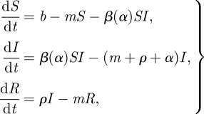2.1

where S is the density of susceptible hosts and I is the density of infective hosts, b is the total birth rate and m the per capita death rate, α is the population mean virulence, ρ is the recovery rate, and β(α) is the transmission rate.

We want to simplify these equations slightly, making several approximations to reduce the number of parameters involved. Let us assume an (approx.) fixed population size N and set b = mN, and assume we can neglect recovery because it is slow and/or unlikely relative to disease-induced mortality (ρ ≪ α). We will also ignore the dynamics of the recovered R individuals, because they do not affect the rest of the epidemic. Then we get

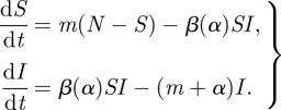2.2

As long as the size of the population does not change significantly over the course of the epidemic, we can relax these simplifying assumptions without changing our conclusions. In the myxomatosis examples below, we set the birth rate greater than the death rate so that host populations would grow exponentially in the absence of the pathogen (Dwyer et al. 1990).

All of our simulations used the lsoda differential equation solver from the deSolve package in R (R Development Core Team 2007; Soetaert et al. 2009; see the electronic supplementary material).

We assume the transmission rate (per susceptible) β is a decelerating function of the clearance/virulence parameter α (i.e. dβ²/d²α < 0); for simplicity we generally use

2.3

with γ > 1 (Frank 1996). Later, we consider the implications of changing the shape of this relationship to a more realistic curve.

As mentioned in §1 (and as usual in tradeoff models of virulence), we define virulence as the rate of disease-induced mortality, which is negatively related to the pathogen's infectious period. While this is a standard definition in the literature, readers should be aware that there are other measures of the harm caused by pathogens (in particular, case mortality or the probability that hosts will die from disease) that may not be associated with shorter infectious periods (Day 2002), and hence will not induce a virulence–transmission tradeoff. If host resistance is relatively weak at the beginning of an epidemic, and it evolves slowly, so that the initial virulence dynamics we see are related to the pathogen's virulence–transmission tradeoff, then our characterization of virulence (and our assumption that recovery, if it occurs, is much slower than disease-induced mortality) may be reasonable.

The dynamical equation for virulence assumes that the change in mean virulence is proportional to the sensitivity of the fitness; the proportionality constant, V_g, is equivalent to the additive genetic variance in a quantitative genetic model (Frank 1996; Abrams 2001). We express the equation in terms of additive genetic variance for simplicity. In comparing evolutionary responses of virulence over a wide range of genetic variability below, we alternatively express variation in terms of the coefficient of variance at the equilibrium virulence (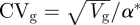)—a unitless measure of variability—as suggested by Houle (1992).

For this model, the fitness of a pathogen strain is the change in the per capita growth rate of infectives per unit change in virulence, or d((dI/dt)/I)/dα. Thus

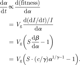2.4

For the model given by equation (2.2), R₀ = β(α)N/(m + α). Some algebra shows that for tradeoff curve (2.3) the equilibrium virulence is

2.5

and the equilibrium value of R₀ is

2.6

2.2. Model parameters

The model represented by equations (2.2)–(2.4) has five parameters (m, N, c, γ, V_g) and three starting values (S(0), I(0), α(0)). We can simplify the model to use only three parameters (γ, c, V) and two starting values (I(0), α(0)), without loss of generality.

First, we assume there are no recovered individuals at the beginning of the epidemic (R(0) = 0), and recognize that therefore S(0) = N − I(0). Second, we set N = 1, scaling c appropriately so that the effective transmission parameter is unchanged. This scaling also means that I(0) is inversely proportional to the population size, because the minimum value of I(0) is 1/N. For example, if the epidemic starts with one infected individual, then I(0) = 10⁻³ corresponds to a population size of 1/I(0) = 1000. Third, we set m = 1 to define the time scale in terms of host mortality rate (or lifespan), so that α is the ratio of the disease-induced mortality rate to the natural mortality rate. For example, if α = 1, then the disease-induced mortality rate is equal to the natural mortality rate and infected individuals live half as long on average (1/(α + m)) as uninfected ones (1/m).

Since we have specified a particular model for the tradeoff curve, we can also reparametrize the model in terms of the disease characteristics at equilibrium. Specifically, we replace the parameters c and γ that describe the shape of the transmission–virulence tradeoff curve with R*₀ and α*, the intrinsic reproductive number and virulence when the pathogen is at both epidemiological and evolutionary equilibrium.

Specifically, substituting m = 1 in equation (2.5) gives

2.7

and from equation (2.6) with m = 1 we get

2.8

Given values of α* and R*₀, we can use these expressions to calculate the corresponding γ and c parameters. For values of γ ≈ 1 (large α*), G(γ) is close to 1. As γ increases to 2 (i.e. α* = 1), G(γ) increases to a maximum of 2, then declines gradually: for large values of γ (α* near 0), G(γ) again approaches 1.

2.3. Model parametrization

We searched for estimates of R₀ and virulence for emerging pathogens with simple natural history and high case mortality, avoiding important but more complex pathogens like tuberculosis, dengue or human malaria (table 1).

Table 1.

Order-of-magnitude estimates for reproductive number (R₀) and virulence (α) for some emerging pathogens. Both parameters are unitless: R₀ is the expected number of secondary cases from a primary case in a completely susceptible population, while α is the disease-induced mortality rate scaled by the natural mortality rate.

pathogen	host	R0	α	reference
SARS	human	3	640	Anderson et al. (2004)
HIV	human	1.43	6.36	Velasco-Hernandez et al. (2002)
WNV	American crow	1.61–3.24	639	Wonham et al. (2004)
myxomatosis	European rabbit	3	5	Dwyer et al. (1990)

We estimated α* as the inverse of the average time to death, scaled by the average host lifespan. For example, the time from onset of SARS symptoms to hospital admission is 2–5 days, and time from admission to death is 36 days (Anderson et al. 2004). Dividing an average human lifespan of 70 years by 40 (= 4 + 36) days gives an α* of 640. The intrinsic reproductive number R₀ (which is unitless) is often estimated for emerging pathogens. We used equations (2.7) and (2.8) to derive c and γ from α* and R*₀. By assuming that the observed R₀ and virulence values for these emerging pathogens are close to the equilibrium values we are contradicting ourselves slightly—if transient virulence is important then these values may overestimate the equilibrium R₀ and underestimate the equilibrium virulence. These estimates should be taken with additional grains of salt because they are based on an extremely simple model, with various strong assumptions (such as a well-mixed, homogeneous, totally susceptible host population, with matching to a single point on a putative tradeoff curve), but our main interest is in order-of-magnitude estimates that will determine if transient virulence could be important.

2.4. Tradeoff curves

Our model assumes not only that a tradeoff exists between virulence and transmission rates, but that it follows a particular form. What do existing data say about the actual shape of the tradeoff curve?

Very few studies answer the critical question of whether the virulence–transmission rate curve decelerates, or in other words whether the total transmission (proportional to R₀) peaks at an intermediate virulence level. Despite the variety of studies that show the existence of a positive correlation between virulence and transmission rates (Ebert 1994; Ebert & Mangin 1997; Lipsitch & Moxon 1997), very few provide enough data to estimate the shape of the tradeoff curve (required in order to apply the tradeoff theory in a quantitative way) or even to determine whether it decelerates. We found only six such studies, covering myxomatosis (Dwyer et al. 1990), Pasteuria ramosa (a parasite of Daphnia magna; Jensen et al. 2006), HIV (Fraser et al. 2007), malaria species infecting mice (Plasmodium chabaudi; Mackinnon & Read 1999a) and chickens (Plasmodium gallinaceum; Paul et al. 2004), and Ophryocystis elektroscirrha (a parasite of monarch butterflies; de Roode et al. 2008). Figure 4 shows the transmission rate as a function of scaled virulence for myxomatosis, P. ramosa, and HIV; the other studies only provide percentages of hosts (or vectors) infected, rather than rates of transmission. (Some data are available for experimental infections of WNV in American crows (Brault et al. 2004), but only one strain (New York 1999) showed high virulence and so the results prove at most that transmission and virulence are positively correlated.)

For myxomatosis (Dwyer et al. 1990), we took the original data from Fenner et al. (1956) and refitted the models from Dwyer et al. (1990) to draw the curve; for P. ramosa we used image analysis software to extract the data from the original paper (fig. 2 of Jensen et al. 2006); and for HIV we used a combination of data provided by C. Fraser (for the relationship between viral load and transmission potential) and data extracted from fig. 2a of Fraser et al. (2007) (relationship between viral load and time to progression). We followed the same fitting procedures as in the original papers. In all cases we derived values for the scaled virulence by dividing the original virulence estimates by the disease-free host lifespan (European rabbit approx. 170 days; Daphnia magna approx. 130 days; humans approx. 70 years).

For the myxomatosis curve (figure 4a), we plot both the curve estimated by Dwyer et al. (1990) and the curve corresponding to the power model (equation (2.3)) with the same equilibrium virulence and total transmission. We also draw the estimated optimal virulence at equilibrium (α* = 4.54, by definition the same for both curves) and the estimated optimal epidemic-phase virulence in a completely susceptible population for the more realistic model (α_epi = 5.16). (The optimal epidemic-phase virulence for the simpler power model falls far to the right of the plotted region (α_epi = 1812); we discuss this below.)

2.5. Genetic variability

Tradeoff curves give only half the information we need to predict transient virulence. The relative time scales of epidemiological and evolutionary dynamics determine whether any evolutionary dynamics will actually be observed in the course of an epidemic: in order to know the time scale, we need to know how much genetic variance for virulence exists in the population (or, if variance is generated dynamically by novel mutations during the course of the epidemic, we need to know the mutation rate and the spectrum of phenotypic consequences).

Many studies have shown that pathogens can evolve rapidly in the wild (Dwyer et al. 1990; Knell 2004) or in the laboratory (Ebert 1998; Mackinnon & Read 1999b, 2004; Mackinnon et al. 2005). However, as with tradeoff curves, such studies rarely give us the data we need to predict transient evolution. Evolutionary studies of model viruses like vesicular stomatitis virus (Moya et al. 2000) usually compete specific strains against each other to determine how fitness (relative growth rate, which may be related to virulence) varies with particular characteristics, but do not estimate the standing variation in the population. Serial passage experiments (Ebert 1998) examine changes in virulence from a mixed starting population, but because they quantify only the response to natural selection, we cannot use them to separate the strength of selection and the genetic variance V_g.

The data on myxomatosis virulence variation shown below belie our assumption of constant genetic variance for virulence (Day & Proulx 2004). We could relax this assumption by driving the model with the observed time-varying values of V_g, or creating a model that tracks the dynamics of the variance in virulence as well as the mean (Turelli 1988), or even model the full distribution of virulence, with variation being constantly generated by novel mutations and eroded by selection. For this study, we chose to retain a simple constant-variance model in order to understand its basic dynamics.

Myxomatosis provides a rare source of data on standing variation in virulence. Myxomatosis was first successfully introduced to Australia in the 1950s as an essentially pure strain, with practically no variation in virulence. Within a few years, however, field collections showed the presence of a variety of different virus grades with varying virulence (Fenner et al. 1956; Dwyer et al. 1990). We combined the data on the proportions of different grades collected with the average time to mortality of each grade (expressed in terms of the host lifespan of approx. 167 days) to compute the variance in virulence over time. After its initial appearance, variance ranged from a low of 2.51 in 1952–1955 (CV_g = 0.26) to a high of 40.79 (CV_g = 0.63) in 1967–1969. In the simulations described below, we used values of V_g = 2.5 (low), 10 (medium), and 40 (high).

Mackinnon & Read (1999a) quantified various proxies of virulence for eight clones of P. chabaudi. Since none of these proxies fit very well with our model of an infectious period truncated by disease-induced mortality—none of the experimental mice died except under anaesthesia-induced stress—we computed only CV_g values for these measures. In the absence of information about the distribution of clones in the wild, we gave all clones equal weight. The CV_g values for Mackinnon & Read's virulence proxies ranged from 0.07 (minimum mouse weight) to 0.58 (parasitemia at the time of maximum gametocytemia), with a mean of 0.39.

2.6. Simulations

Our basic simulation protocol starts the system with a low pathogen prevalence, the rest of the population susceptible and virulence set to its equilibrium value (α(0) = α*), mimicking the emergence of a novel pathogen that was previously in epidemiological–evolutionary equilibrium.

We ran factorial combinations over the free parameters of initial epidemic size (I(0) = {10⁻⁴, 10⁻³, 10⁻²}), genetic variance V (expressed as a coefficient of variation: CV_g = {0.1, 0.5, 1}), equilibrium R₀ (ranging from 1.1 to 50), and α* (ranging from 1 to 1000).

3. Results

3.1. Basic simulations

Numerical simulations (figure 1) confirm the expected properties of the model: prevalence increases from its low starting value up to a stable equilibrium, while average virulence increases up to a transient peak and then declines. Since the starting value is set to the ecological–evolutionary equilibrium, final virulence is the same as starting virulence. The epidemic always reaches a stable equilibrium prevalence and average virulence (provided that R*₀ > 1).

Figure 1.

Basic epidemic–evolutionary dynamics of an emerging pathogen. Black line (left axis) shows the fraction of the host population infective (prevalence) over time; grey line (right axis) shows the average virulence of the pathogen population over time. Black arrow shows the peak time t̂, expressed as a prevalence (see main text); grey arrow shows the peak virulence α̂, relative to the equilibrium virulence. Parameters: V_g = 5, c = 3, γ = 2 (R*₀ = 1.5, α* = 1); starting conditions I(0) = 0.001, S(0) = 0.999, α(0) = α* = 1.

Figure 1 also illustrates the summary measures we use to describe the results from simulations with a particular set of parameters. In this case, the virulence increases by a factor of α̂ = 2.12 over its initial value (which happens to be 1 in this case). The peak occurs when prevalence has risen to t̂ = 9.03 per cent of its maximum value.

3.2. Factorial simulations

What about the results over a wider swath of parameter space (figure 2)? Our main response variable is the height of the transient peak in virulence, scaled relative to the equilibrium virulence (α̂). We also recorded the timing of the transient peak (t̂), expressed as the ratio of disease prevalence at the time of maximum virulence to the maximum prevalence. This peak ‘time’ gives a unitless measure of the fraction of the epidemic that has occurred when the virulence peaks.

Figure 2.

Peak virulence α̂, scaled by equilibrium virulence, across a range of parameters. Axes within subfigures: equilibrium R*₀ (horizontal), equilibrium virulence α* (vertical). Subfigures: starting prevalence I(0) (horizontal), genetic coefficient of variation in virulence CV_g (vertical). Solid contours range from 1.5 to 4 in steps of 0.5; dashed contours (shown only in bottom row, for CV_g = 0.1) range from 1 to 1.5 in steps of 0.025. Middle figure shows the location of emerging pathogens from table 1 with respect to R*₀ and α* (genetic variability and initial prevalence are unknown for these pathogens). (Horizontal positions of WNV and SARS are displaced slightly for legibility.)

Figure 2 shows that the transient peak can be quite large (more than four times the equilibrium virulence), but it depends very strongly on the degree of genetic variability. The peak virulence increases with decreasing starting prevalence I(0) (rightmost subplots), increasing R*₀ (right edge of subplots), increasing equilibrium virulence α* (top edge of subplots) and most strongly with increasing variability CV_g (topmost subplots). When CV_g = 1, the peak virulence is generally large (1.5–4 times equilibrium virulence) and depends strongly on the other three parameters (I(0), R*₀ and α*). With intermediate variance (CV_g = 0.5), virulence increases by more than 50 per cent over a wide range of parameters and can more than double for high-R*₀, high-virulence pathogens such as SARS. When CV_g = 0.1, virulence never increases by more than a few percent over its equilibrium value.

However, the timing of peak virulence t̂ (figure 3) may contradict our hypothesis that virulence evolution contributes to the apparently high virulence of emerging pathogens. Except for low-R*₀, low-α* pathogens, the peak of virulence does not occur until the epidemic has nearly reached its peak (t̂ > 0.99 over most of parameter space). Thus, unless the emerging pathogen went undetected until it was already starting to decrease, epidemiologists would observe a phase of increasing virulence at the beginning of an emerging epidemic, rather than seeing a level of virulence that had already been inflated by transient selection and was now decreasing.

Figure 3.

Peak time t̂. Axes and parameter ranges as in figure 2. Contour lines at t̂ = {0.5,0.9,0.99}.

Running the model with the birth rate set to zero, to simulate the dynamics of an epidemic in a slowly reproducing host (i.e. simulating a more familiar ‘SIR’-type epidemic where the epidemic declines as susceptibles are exhausted) gives similar results to those shown above. The only qualitative difference is that virulence peaks at a lower value when R*₀ and α* are low.

3.3. Tradeoff curves

What can we say about the true shapes of the tradeoff curves, in the few cases where we can quantify them (figure 4)? All three pathogens (myxomatosis, Pasteuria ramosa and HIV) show decelerating curves (∂²β/∂α² < 0) overall, as required by the tradeoff theory in order for a stable equilibrium virulence to exist. The HIV tradeoff curve accelerates at low virulence (α < 3) and may accelerate slightly when α > 20 (although the confidence intervals are extremely wide in this region). For myxomatosis and Pasteuria ramosa, the transmission rate actually decreases for high virulence (rather than simply decelerating). There is no particular reason to expect this shape—on the basis of a simple within-host model with plausible parameter values, Alizon & van Baalen (2005) suggested only decelerating, and not decreasing, transmission rates with increasing virulence. The effect of a decreasing tradeoff curve (as will be demonstrated below) is to limit the magnitude of the transient peak in virulence, because high virulences that would be expected to lead to rapid population growth under the simplest tradeoff curve (equation (2.3)) will instead be maladaptive.

Figure 4.

Tradeoff curves: shaded areas show 95% confidence envelopes in all cases. (a) Myxomatosis in European rabbits (Dwyer et al. 1990). Solid curve, estimated tradeoff curve; dashed curve, tradeoff curve based on equation (2.3) with equivalent equilibrium virulence α*. Vertical lines show (solid) equilibrium virulence and (dotted) optimal epidemic virulence for the more realistic tradeoff curve. (b) Pasteuria ramosa in Daphnia magna (Jensen et al. 2006): fit of a quadratic generalized linear model. (c) HIV in humans (Fraser et al. 2007).

3.4. Myxomatosis simulations

Using our best estimates of the parameters for myxomatosis, with the general theoretical model (equation (2.3)) and our medium (V_g = 10) and high (V_g = 40) estimates of variance, the simulations capture the observed virulence dynamics of Australian myxomatosis reasonably well (figure 5a). The discrepancies in the fit seem quite reasonable given the fact that the model uses only individual-level information derived from the experiments reported in Fenner et al. (1956): the mean and variance in the virulence are the only parameters estimated from field measurements. The model is also (intentionally) very simple: in particular, V_g is held constant at various values rather than being allowed to vary over time.

Figure 5.

Myxomatosis simulations using different genetic variances (V_g) and different tradeoff curves. ‘Power’ curve refers to the general theoretical curve (equation (2.3), dashed line in figure 4a), ‘realistic’ curve refers to the myxomatosis-specific curve (solid line in figure 4a). (a) Starting virulence equal to observed 1950 value (α = 25.6). Horizontal grey bars show average observed virulence over time. (b) Starting virulence equal to expected equilibrium virulence (α = 4.5). Note scale difference: the range of (b) includes the grey box in the lower left corner of (a). Dashed black line, V_g = 2.5; thick black line, V_g = 10; dotted black line, V_g = 40 (power). Dashed grey line, V_g = 2.5; grey line, V_g = 10; dotted grey line, V_g = 40 (realistic).

The observed virulence never drops all the way to the expected equilibrium level, and in fact appears to rebound slightly towards the end of the period. Dwyer et al. (1990) interpreted these changes as a coevolutionary pathogen response to increasing host immunity (Mackinnon & Read (2004) found similar results in experiments on P. chabaudi in mice): since our model does not include changes in host immunity, it cannot respond in this way.

If we use instead the more realistic, myxomatosis-specific tradeoff curve from figure 4a, virulence declines much more rapidly than observed—especially with high genetic variance. This steep drop in transmission is caused by strong selection against high virulence, much stronger than with the simpler power-law tradeoff curve. For myxomatosis, high virulence does not just decrease total transmission (transmission rate multiplied by infectious period), but actually decreases transmission rate, rather than just slowing its growth as required by the tradeoff model. We do not know why the model with the more realistic virulence curve matches the data so poorly, although (among other simplifications) this simulation predicts changes in virulence in a single homogeneously mixed population whereas the data come from field samples spread across Australia. Allowing virulence to decrease over time would generally slow the rate of convergence to the equilibrium virulence, although in this case the virulence drops too rapidly even at the lowest level of virulence (V_g = 2.5, slightly below the observed minimum estimate that occurred for 1967–1969). (In general, the results of decreasing virulence could have a variety of effects on virulence dynamics, either prolonging or damping out the transient peak of virulence, depending on the relative timing of the decrease in virulence.)

Figure 5b shows the hypothetical results of a myxomatosis outbreak with the same parameters as figure 5a but with a starting virulence equal to the equilibrium virulence instead of the high virulence selected for biocontrol. This simulation mimics what one might have seen if myxomatosis had emerged naturally, for example from a population of introduced rabbits carrying myxomatosis. In this case, the power-law tradeoff predicts that virulence would increase rapidly, reaching transient peaks of 29 per cent (V_g = 2.5), 90 per cent (V_g = 10), or 216 per cent (V_g = 40) above its starting level. These peaks occur rapidly, within the first six months of the epidemic. The virulence trajectories cross, so that the least evolvable pathogen (V_g = 2.5) also takes longest to drop back to its equilibrium virulence.

For the more realistic model, the transient virulence is much more constrained, with increases between 11 per cent (V_g = 2.5) and 14 per cent (V_g = 10 or 40). Because high virulence decreases transmission rate and not just total transmission, the transient virulence is mostly limited by the tradeoff curve itself, rather than by a combination of the tradeoff curve and the window of opportunity for epidemic selection. Thus, manipulating the epidemic in other ways to increase the scope for transient selection, such as decreasing initial prevalence or increasing genetic variance still further, gives no additional increase in the transient peak. (While one might argue from this lack of response with the more realistic tradeoff curve that large transient virulence peaks are just an artefact of the simpler model, we note that the more realistic model also predicts an unrealistically rapid drop in the virulence in figure 5a.)

4. Discussion

Our simple dynamic tradeoff model of epidemiological and evolutionary pathogen dynamics (Day & Proulx 2004), using parameters estimated for a handful of emerging pathogens, suggests that transient epidemic-phase selection can indeed drive significant increases in pathogen virulence. The critical parameter of genetic variability V_g is largely unknown, but for the two examples we can quantify variance (measured as CV_g) varies from approximately 0.4 to 0.6—in the intermediate, and potentially important, range (figure 2, middle row).

Our myxomatosis simulations point to the importance of both evolutionary constraints (genetic variance) and epidemiological or physiological constraints (the tradeoff curve). Our myxomatosis simulations simplify a complex natural system, and incorporate a fairly narrow range of the possible mechanisms operating. Sabelis & Metz (2002) list seven mechanisms, including within-host competition, coevolution of pathogen virulence and host immunity, and selection at the level of rabbit family groups, of which our model only allows two (virulence–transmission tradeoffs at the level of an infected host and effects of changing population size). On the other hand, we are encouraged that a model which is based only on individual level parameters, and which is even more of a caricature than the model of Dwyer et al. (1990), comes reasonably close—although the failure of the more realistic tradeoff curve to accurately model virulence dynamics definitely leaves an open question.

If total transmission decreases while transmission rate remains high (as in the case of HIV), then a large transient spike in virulence seems likely. On the other hand, if the virulence–transmission tradeoff curve drops off so rapidly that both transmission rate and total transmission decrease at high virulence (as in the cases of myxomatosis and P. ramosa), transient virulence may be damped out by strong selection against high virulence. Because tradeoff curves are so rarely measured, we can only speculate as to which case is more typical.

4.1. Implications for virulence evolution theory

While the tradeoff theory was the first rigorous model of the evolution of virulence in a host–pathogen system, some have complained that it has outstripped its empirical underpinnings (Levin & Bull 1994; Ebert & Bull 2003). The most compelling empirical studies have tested qualitative differences in virulence as a function of mode of transmission, rather than investigating the quantitative changes in virulence with variation in transmission rates or epidemiological context (Bull et al. 1991; Herre 1995; Ebert 1999; Messenger et al. 1999).

More recently, both theoreticians and empiricists have shifted away from the between-host level of selection represented by the tradeoff theory to explore within-host selection more carefully (Antia & Lipsitch 1997; Davies et al. 2002; Alizon & van Baalen 2005; André & Gandon 2006; André & Godelle 2006; Bell et al. 2006; Brown et al. 2006). Part of this shift comes from realizing the potential importance of within-host dynamics, but we believe that part also comes from the temptation to shift our attention to phenomena we can measure more easily. Working on within-host dynamics allows empiricists to run well-replicated experiments on multiple hosts and gives them access to molecular and biomedical techniques. These capabilities in turn give theoreticians a rich vein of information to use in testing and parametrizing both qualitative and mechanistic models.

The best available data on the transmission–virulence tradeoff come from vector- or waterborne pathogens, where researchers can measure proxies for transmission like gametocytemia or propagule production (Dwyer et al. 1990; Mackinnon & Read 1999a; Paul et al. 2004; Jensen et al. 2006). One problem with such transmission proxies is that nonlinearities in the relationship between proxies and actual transmission could significantly alter the shape of the tradeoff curve and hence the predictions of the tradeoff theory. Despite the uncertainty in the relationship between proxies and transmission, and the complexity of vector biology, these systems have yielded more information on virulence and transmission than airborne or fomite-transmitted pathogens.

With a few exceptions (Kerr et al. 2006; Boots & Mealor 2007), however, empiricists have been unable to control and manipulate transmission in order to test the tradeoff theory rigorously. While the details of the model would have to be adapted to specific experimental systems, we think that the predictions explored here should be eminently testable in microbial systems, perhaps using separate strains with distinct virulences rather than a pathogen with a continuous spectrum of virulence for tractability.

Observing virulence dynamics in the wild is far more difficult. There has been a decade and a half of debate over the expected trajectory of virulence evolution in HIV (Ewald 1991; Bonhoeffer & Nowak 1994; Lipsitch & Nowak 1995; Massad 1996; Lipsitch 1997; Coutinho et al. 1999; Levin et al. 2001; Courgnaud et al. 2004). While recent studies suggest that subtypes with lower fitness now dominate, the empirical evidence on the trajectory of virulence is still somewhat ambiguous (Ariën et al. 2005, 2007; Müller et al. 2006, 2009; Herbeck et al. 2008)—perhaps not surprising given the complexity of HIV, which has multiple subtypes, inhabiting many genotypes of hosts, multiple tissue types, and with hugely variable ecological and evolutionary pressures at different stages of infection of a single host.

While HIV—with its slow dynamics, lack of small-animal models and immunological complexity—may represent a worst-case scenario for understanding virulence evolution, studies as far back as the 1940s (Topley 1942) have explored the ecology of transmission in the laboratory. Such experiments are also possible in evolutionary contexts (Kerr et al. 2006; Boots & Mealor 2007). The biggest challenge, however, will be combining molecular, physiological, immunological and epidemiological levels to understand and predict the evolutionary trajectory of pathogens in the wild. Model systems will help (Mackinnon & Read 1999a; Paul et al. 2004); so will the development of reliable transmission proxies for a wider range of host–pathogen systems.

Our models demonstrate a mechanism that could be responsible for doubling the virulence of emerging pathogens, but our main conclusion from parametrizing these models is that we still lack the quantitative information on pathogen characteristics that would tell us how important these phenomena are for understanding and managing emerging pathogens in the real world. As Alizon et al. (2009) state, ‘[t]hat some evidence to support the trade-off hypothesis is lacking is more of a call to improve the theory and experiments than to discard it’. We stress that our models are simple and strategic, leaving out many undoubtedly important facets of epidemiology and host–pathogen evolution (especially within-host competition, host–pathogen coevolution, and details of pathogen life history). However, based on the evidence we have been able to gather we conclude that virulence–transmission tradeoffs could play a large role in driving the virulence of emerging pathogens.

References

- Abrams P. A. 2001. Modelling the adaptive dynamics of traits involved in inter- and intraspecific interactions: an assessment of three methods. Ecol. Lett. 4, 166–175. ( 10.1046/j.1461-0248.2001.00199.x) [DOI] [Google Scholar]
- Alizon S., van Baalen M. 2005. Emergence of a convex trade-off between transmission and virulence. Am. Nat. 165, E155–E167. ( 10.1086/430053) [DOI] [PubMed] [Google Scholar]
- Alizon S., Hurford A., Mideo N., van Baalen M. 2009. Virulence evolution and the trade-off hypothesis: history, current state of affairs and the future. J. Evol. Biol. 22, 245–259. ( 10.1111/j.1420-9101.2008.01658.x) [DOI] [PubMed] [Google Scholar]
- Anderson R. M., Fraser C., Ghani A. C., Donnelly C. A., Riley S., Ferguson N. M., Leung G. M., Lam T. H., Hedley A. J. 2004. Epidemiology, transmission dynamics, and control of SARS: the 2002–2003 epidemic. Phil. Trans. R. Soc. Lond. B 359, 1091–1105. ( 10.1098/rstb.2004.1490) [DOI] [PMC free article] [PubMed] [Google Scholar]
- André J. B., Gandon S. 2006. Vaccination, within-host dynamics, and virulence evolution. Evolution 60, 13–23. ( 10.1111/j.0014-3820.2006.tb01077.x) [DOI] [PubMed] [Google Scholar]
- André J. B., Godelle B. 2006. Within-host evolution and virulence in microparasites. J. Theor. Biol. 241, 402–409. ( 10.1016/j.jtbi.2005.12.011) [DOI] [PubMed] [Google Scholar]
- André J., Hochberg M. E. 2005. Virulence evolution in emerging infectious diseases. Evolution 59, 1406–1412. ( 10.1111/j.0014-3820.2005.tb01791.x) [DOI] [PubMed] [Google Scholar]
- Antia R., Lipsitch M. 1997. Mathematical models of parasite responses to host immune defences. Parasitology 115, S155–S167. ( 10.1017/S003118209700200X) [DOI] [PubMed] [Google Scholar]
- Ariën K. K., Troyer R. A., Gali Y., Colebunders R. L., Arts E. J., Vanham G. 2005. Replicative fitness of historical and recent HIV-1 isolates suggests HIV-1 attenuation over time. AIDS 19, 1555–1564. ( 10.1097/01.aids.0000185989.16477.91) [DOI] [PubMed] [Google Scholar]
- Ariën K. K., Vanham G., Arts E. J. 2007. Is HIV-1 evolving to a less virulent form in humans? Nat. Rev. Microbiol. 5, 141–151. ( 10.1038/nrmicro1594) [DOI] [PMC free article] [PubMed] [Google Scholar]
- Beck M. A., Handy J., Levander O. A. 2004. Host nutritional status: the neglected virulence factor. Trends Microbiol. 12, 417–423. ( 10.1016/j.tim.2004.07.007) [DOI] [PMC free article] [PubMed] [Google Scholar]
- Bell A. S., De Roode J. C., Sim D., Read A. F. 2006. Within-host competition in genetically diverse malaria infections: Parasite virulence and competitive success. Evolution 60, 1358–1371. ( 10.1111/j.0014-3820.2006.tb01215.x) [DOI] [PubMed] [Google Scholar]
- Bonhoeffer S., Nowak M. A. 1994. Mutation and the evolution of virulence. Proc. R. Soc. Lond. B 258, 133–140. ( 10.1098/rspb.1994.0153) [DOI] [Google Scholar]
- Boots M., Mealor M. 2007. Local interactions select for lower pathogen infectivity. Science 315, 1284–1286. ( 10.1126/science.1137126) [DOI] [PubMed] [Google Scholar]
- Brault A. C., Langevin S. A., Bowen R. A., Panella N. A., Biggerstaff B. J., Miller B. R., Komar N. 2004. Differential virulence of West Nile strains for American crows. Emerg. Inf. Dis. 10, 2161–2168. [DOI] [PMC free article] [PubMed] [Google Scholar]
- Brown S. P., Cornell S. J., Sheppard M., Grant A. J., Maskell D. J., Grenfell B. T., Mastroeni P. 2006. Intracellular demography and the dynamics of Salmonella enterica infections. PLoS Biol. 4, e349 ( 10.1371/journal.pbio.0040349) [DOI] [PMC free article] [PubMed] [Google Scholar]
- Bull J. J., Ebert D. 2008. Invasion thresholds and the evolution of nonequilibrium virulence. Evol. Appl. 1, 172–182. ( 10.1111/j.1752-4571.2007.00003.x) [DOI] [PMC free article] [PubMed] [Google Scholar]
- Bull J. J., Molineux I. J., Rice W. R. 1991. Selection of benevolence in a host–parasite system. Evolution 45, 875–882. ( 10.2307/2409695) [DOI] [PubMed] [Google Scholar]
- Courgnaud V., Müller-Trutwin M., Sonigo P. 2004. Evolution and virulence of primate lentiviruses. Medicine/Sciences 20, 448–452. [DOI] [PubMed] [Google Scholar]
- Coutinho F. A. B., Massad E., Menezes R. X., Burattini M. N. 1999. A theoretical model of the evolution of virulence in sexually transmitted HIV/AIDS. Rev. Saude Publ. 33, 329–333. ( 10.1590/S0034-89101999000400002) [DOI] [PubMed] [Google Scholar]
- Davies C. M., Fairbrother E., Webster J. P. 2002. Mixed strain schistosome infections of snails and the evolution of parasite virulence. Parasitology 124, 31–38. ( 10.1017/S0031182001008873) [DOI] [PubMed] [Google Scholar]
- Day T. 2002. On the evolution of virulence and the relationship between various measures of mortality. Proc. R. Soc. Lond. B 269, 1317–1323. ( 10.1098/rspb.2002.2021) [DOI] [PMC free article] [PubMed] [Google Scholar]
- Day T., Proulx S. R. 2004. A general theory for the evolutionary dynamics of virulence. Am. Nat. 163, E40–E63. ( 10.1086/382548) [DOI] [PubMed] [Google Scholar]
- de Roode J. C., Yates A. J., Altizer S. 2008. Virulence–transmission trade-offs and population divergence in virulence in a naturally occurring butterfly parasite. Proc. Natl Acad. Sci. USA 105, 7489–7494. ( 10.1073/pnas.0710909105) [DOI] [PMC free article] [PubMed] [Google Scholar]
- Dieckmann U., Metz J. A. J., Sabelis M. W., Sigmund K. (eds) 2002. Adaptive dynamics of infectious diseases: in pursuit of virulence management. Cambridge, UK: Cambridge University Press. [Google Scholar]
- Dwyer G., Levin S., Buttel L. 1990. A simulation model of the population dynamics and evolution of myxomatosis. Ecol. Monogr. 60, 423–447. ( 10.2307/1943014) [DOI] [Google Scholar]
- Ebert D. 1994. Virulence and local adaptation of a horizontally transmitted parasite. Science 265, 1084–1086. ( 10.1126/science.265.5175.1084) [DOI] [PubMed] [Google Scholar]
- Ebert D. 1998. Experimental evolution of parasites. Science 282, 1432–1435. ( 10.1126/science.282.5393.1432) [DOI] [PubMed] [Google Scholar]
- Ebert D. 1999. The evolution and expression of parasite virulence. In Evolution in health & disease (ed. Stearns S. C.), ch. 14, pp. 161–172. Oxford, UK: Oxford University Press. [Google Scholar]
- Ebert D., Bull J. J. 2003. Challenging the trade-off model for the evolution of virulence: is virulence management feasible? Trends Microbiol. 11, 15–20. ( 10.1016/S0966-842X(02)00003-3) [DOI] [PubMed] [Google Scholar]
- Ebert D., Mangin K. L. 1997. The influence of host demography on the evolution of virulence of a microsporidian gut parasite. Evolution 51, 1828–1837. ( 10.2307/2411005) [DOI] [PubMed] [Google Scholar]
- Ewald P. W. 1991. Transmission modes and the evolution of virulence, with special reference to cholera, influenza, and AIDS. Hum. Nat. 2, 1–30. ( 10.1007/BF02692179) [DOI] [PubMed] [Google Scholar]
- Fenner F., Day M. F., Woodroofe G. M. 1956. Epidemiological consequences of the mechanical transmission of myxomatosis by mosquitoes. J. Hyg. (London) 54, 284–302. ( 10.1017/S0022172400044521) [DOI] [PMC free article] [PubMed] [Google Scholar]
- Frank S. A. 1996. Models of parasite virulence. Q. Rev. Biol. 71, 37–78. ( 10.1086/419267) [DOI] [PubMed] [Google Scholar]
- Fraser C., Hollingsworth T. D., Chapman R., de Wolf F., Hanage W. P. 2007. Variation in HIV-1 set-point viral load: epidemiological analysis and an evolutionary hypothesis. Proc. Natl Acad. Sci. USA 104, 17 441–17 446. ( 10.1073/pnas.0708559104) [DOI] [PMC free article] [PubMed] [Google Scholar]
- Gilchrist M. A., Coombs D. 2006. Evolution of virulence: interdependence, constraints, and selection using nested models. Theor. Popul. Biol. 69, 145–153. ( 10.1016/j.tpb.2005.07.002) [DOI] [PubMed] [Google Scholar]
- Herbeck J. T., Gottlieb G. S., Li X., Hu Z., Detels R., Phair J., Rinaldo C., Jacobson L. P., Margolick J. B., Mullins J. I. 2008. Lack of evidence for changing virulence of HIV-1 in North America. PLoS ONE 3, e1525 ( 10.1371/journal.pone.0001525) [DOI] [PMC free article] [PubMed] [Google Scholar]
- Herre E. A. 1995. Factors affecting the evolution of virulence: nematode parasites of fig wasps as a case study. Parasitology 111, S179–S191. ( 10.1017/S0031182000075880) [DOI] [Google Scholar]
- Houle D. 1992. Comparing evolvability and variability of quantitative traits. Genetics 130, 195–204. [DOI] [PMC free article] [PubMed] [Google Scholar]
- Jensen K. H., Little T., Skorping A., Ebert D. 2006. Empirical support for optimal virulence in a castrating parasite. PLoS Biol. 4, e197 ( 10.1371/journal.pbio.0040197) [DOI] [PMC free article] [PubMed] [Google Scholar]
- Johnston S. 1987. Epidemics: the forgotten factor in seventeenth century warfare in the St. Lawrence region. In Native peoples, native lands (ed. Cox B. A.), ch. 2, pp. 14–31. Montreal, Canada: McGill-Queen's University Press. [Google Scholar]
- Kerr B., Neuhauser C., Bohannan B. J. M., Dean A. M. 2006. Local migration promotes competitive restraint in a host–pathogen ‘tragedy of the commons’. Nature 442, 75–78. ( 10.1038/nature04864) [DOI] [PubMed] [Google Scholar]
- Knell R. J. 2004. Syphilis in Renaissance Europe: rapid evolution of an introduced sexually transmitted disease? Proc. R. Soc. Lond. B 271, S174–S176. ( 10.1098/rsbl.2003.0131) [DOI] [PMC free article] [PubMed] [Google Scholar]
- Lenski R. E., May R. M. 1994. The evolution of virulence in parasites and pathogens: reconciliation between two competing hypotheses. J. Theor. Biol. 169, 253–265. ( 10.1006/jtbi.1994.1146) [DOI] [PubMed] [Google Scholar]
- Levin B. R., Bull J. J. 1994. Short-sighted evolution and the virulence of pathogenic microorganisms. Trends Microbiol. 2, 76–81. ( 10.1016/0966-842X(94)90538-X) [DOI] [PubMed] [Google Scholar]
- Levin B. R., Svanborg-Eden C. 1990. Selection and the evolution of virulence in bacteria: an ecumenical excursion and modest suggestion. Parasitology 100, S103–115. ( 10.1017/S0031182000073054) [DOI] [PubMed] [Google Scholar]
- Levin B. R., Bull J. J., Stewart F. M. 2001. Epidemiology, evolution, and future of the HIV/AIDS pandemic. Emerg. Inf. Dis. 7, 505–511. ( 10.3201/eid0703.010305) [DOI] [PMC free article] [PubMed] [Google Scholar]
- Levin S., Pimentel D. 1981. Selection of intermediate rates of increase in parasite-host systems. Am. Nat. 117, 308–315. ( 10.1086/283708) [DOI] [Google Scholar]
- Lipsitch M. 1997. Transmission rates and HIV virulence: comments. Evolution 51, 319–320. ( 10.2307/2410988) [DOI] [PubMed] [Google Scholar]
- Lipsitch M., Moxon E. R. 1997. Virulence and transmissibility of pathogens: what is the relationship? Trends Microbiol. 5, 31–37. ( 10.1016/S0966-842X(97)81772-6) [DOI] [PubMed] [Google Scholar]
- Lipsitch M., Nowak M. A. 1995. The evolution of virulence in sexually-transmitted HIV/AIDS. J. Theor. Biol. 174, 427–440. ( 10.1006/jtbi.1995.0109) [DOI] [PubMed] [Google Scholar]
- Mackinnon M. J., Read A. F. 1999a. Genetic relationships between parasite virulence and transmission in the rodent malaria Plasmodium chabaudi. Evolution 53, 689–703. ( 10.2307/2640710) [DOI] [PubMed] [Google Scholar]
- Mackinnon M. J., Read A. F. 1999b. Selection for high and low virulence in the malaria parasite Plasmodium chabaudi. Proc. R. Soc. Lond. B 266, 741–748. ( 10.1098/rspb.1999.0699) [DOI] [PMC free article] [PubMed] [Google Scholar]
- Mackinnon M. J., Read A. F. 2004. Immunity promotes virulence evolution in a malaria model. PLoS Biol. 2, e230 ( 10.1371/journal.pbio.0020230) [DOI] [PMC free article] [PubMed] [Google Scholar]
- Mackinnon M. J., Bell A., Read A. F. 2005. The effects of mosquito transmission and population bottlenecking on virulence, multiplication rate and rosetting in rodent malaria. Int. J. Parasitol. 35, 145–153. ( 10.1016/j.ijpara.2004.11.011) [DOI] [PubMed] [Google Scholar]
- Massad E. 1996. Transmission rates and the evolution of HIV virulence. Evolution 50, 916–918. ( 10.2307/2410863) [DOI] [PubMed] [Google Scholar]
- Messenger S. L., Molineux I. J., Bull J. J. 1999. Virulence evolution in a virus obeys a trade-off. Proc. R. Soc. Lond. B 266, 397–404. ( 10.1098/rspb.1999.0651) [DOI] [PMC free article] [PubMed] [Google Scholar]
- Moya A., Elena S. F., Bracho A., Miralles R., Barrio E. 2000. The evolution of RNA viruses: a population genetics view. Proc. Natl Acad. Sci. USA 97, 6967–6973. ( 10.1073/pnas.97.13.6967) [DOI] [PMC free article] [PubMed] [Google Scholar]
- Müller V., et al. 2006. Stable virulence levels in the HIV epidemic of Switzerland over two decades. AIDS 20, 889–894. ( 10.1097/01.aids.0000218553.51908.6b) [DOI] [PubMed] [Google Scholar]
- Müller V., et al. 2009. Increasing clinical virulence in two decades of the Italian HIV epidemic. PLoS Pathogens 5, e1000454 ( 10.1371/journal.ppat.1000454) [DOI] [PMC free article] [PubMed] [Google Scholar]
- Paul R. E. L., Lafond T., Muller-Graf C. D. M., Nithiuthai S., Brey P. T., Koella J. C. 2004. Experimental evaluation of the relationship between lethal or non-lethal virulence and transmission success in malaria parasite infections. BMC Evol. Biol. 4, 30 ( 10.1186/1471-2148-4-30) [DOI] [PMC free article] [PubMed] [Google Scholar]
- R Development Core Team. 2007. R: a language and environment for statistical computing. R Foundation for Statistical Computing, Vienna, Austria. See http://www.R-project.org. [Google Scholar]
- Sabelis M. W., Metz J. A. J. 2002. Taking stock: relating theory to experiment. In Adaptive dynamics of infectious diseases: in pursuit of virulence management (eds Dieckmann U., Metz J. A. J., Sabelis M. W., Sigmund K.), pp. 379–398. Cambridge, UK: Cambridge University Press. [Google Scholar]
- Sarkar D. 2009. lattice: lattice graphics. See http://CRAN.R-project.org/package=lattice. R package version 0.17-25. [Google Scholar]
- Sarkar D., Andrews F. 2009. latticeExtra: extra graphical utilities based on lattice. See http://CRAN.R-project.org/package=latticeExtra. R package version 0.6-1. [Google Scholar]
- Soetaert K., Petzoldt T., Setzer R. W. 2009. deSolve: general solvers for initial value problems of ordinary differential equations (ODE), partial differential equations (PDE) and differential algebraic equations (DAE). See http://CRAN.R-project.org/package=deSolve. R package version 1.3. [Google Scholar]
- Topley W. W. C. 1942. The Croonian lecture: the biology of epidemics. Proc. R. Soc. Lond. B 130, 337–359. ( 10.1098/rspb.1942.0005) [DOI] [Google Scholar]
- Turelli M. 1988. Phenotypic evolution, constant covariances, and the maintenance of additive variance. Evolution 42, 1342–1347. ( 10.2307/2409017) [DOI] [PubMed] [Google Scholar]
- Velasco-Hernandez J. X., Gershgorn H. B., Blower S. M. 2002. Could widespread use of combination antiretroviral therapy eradicate HIV epidemics? Lancet 2, 487–493. ( 10.1016/S1473-3099(02)00346-8) [DOI] [PubMed] [Google Scholar]
- Wonham M. J., de Camino-Beck T., Lewis M. A. 2004. An epidemiological model for West Nile virus: invasion analysis and control applications. Proc. R. Soc. Lond. B 271, 501–507. ( 10.1098/rspb.2003.2608) [DOI] [PMC free article] [PubMed] [Google Scholar]
- Woolhouse M. E. J., Haydon D. T., Antia R. 2005. Emerging pathogens: the epidemiology and evolution of species jumps. Trends Ecol. Evol. 20, 238–244. ( 10.1016/j.tree.2005.02.009) [DOI] [PMC free article] [PubMed] [Google Scholar]