Regional Analysis of Self-Reported Personality Disorder Criteria

Abstract

Building on the theoretical work of Louis Guttman, we propose that the core problem facing research into the multidimensional structure of the personality disorders is not the identification of factorial simple structure but rather detailed characterization of the multivariate configuration of the diagnostic criteria. Dimensions rotated to orthogonal or oblique simple structure are but one way out of many to characterize a multivariate map, and their current near universal application represents a choice for a very particular set of interpretive advantages and disadvantages. We use multidimensional scaling and regional interpretation to investigate the structure of 78 self-reported personality disorder criteria from a large sample of military recruits and college students. Results suggest that the criteria have a three-dimensional radex structure that conforms only loosely to the 10 existing personality disorder (PD) categories. Regional interpretation in three dimensions elucidates several important aspects of PDs and their interrelationships.

We cannot do justice to the characteristics of the mind by linear outlines like those in a drawing or in primitive painting, but rather by areas of colour melting into one another as they are presented by modern artists. After making the separation we must allow what we have separated to merge together once more. You must not judge too harshly a first attempt at giving a pictorial representation of something so intangible as psychical processes.

——Freud (1933), New Introductory Lectures in Psychoanalysis

The Characterization of Maps

Figure 1 is a map studied by every schoolchild in Virginia. It depicts the state divided into five regions: Tidewater, Piedmont, Blue Ridge, Valley and Ridge, and Appalachian Plateau. There can be little doubt that a map of this kind contains useful information for someone who wishes to understand the topography of the state, but what exactly is the nature of that information? We can immediately note several characteristics. First of all, the lines that have been drawn between the regions are to some degree arbitrary. It is not a matter of scientific inquiry where precisely the boundary between the Tidewater region and the Piedmont should be drawn; rather, it is a question of convenience and utility. Nevertheless, it would be incorrect to say that the locations of the boundaries are completely arbitrary or the areas they define completely meaningless. The word region combines these characteristics of meaningful contiguity and arbitrary boundary. We can talk about the Piedmont region of Virginia because the locations it contains share characteristics that are not shared by locations in other regions. We will refer to regions of this kind as meaningful but arbitrary, or MBA.

Figure 1.

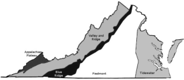
Regionalized map of Virginia.

A second characteristic of the map is that it is based on the subdivision of the state into geometrically defined shapes despite the obvious fact that the geographical space it describes is thoroughly continuous. The choice of a regionally based system of shapes is presumably not justified by an unrealistic belief in actual discontinuities between regions. Once again, the state is divided as it is because it suits our practical purposes to do so. It is particularly interesting that we adopt this strategy despite the ready availability of a familiar alternative that would appear to have many advantages: The Cartesian (actually spherical, but we can ignore that temporarily while we work with two-dimensional maps) system of latitude and longitude. Like geometric space, latitudes and longitudes are continuous, and they have the additional advantage of being numerical rather than geometric. Why don't children learn about the Commonwealth in terms of latitude and longitude?

Consider the question: Where are the mountains in Virginia? They are in the western part of the state, certainly, but looking at Figure 1 we can say more than that. They are in an arc along the western boundary of the state, running from southwest to northeast. We can run our finger along the Blue Ridge, and say, “They are about here.” The point is not that it is impossible to characterize precisely the location of the mountains using latitude and longitude. “West” refers to a direction in longitude, and though it is a little less clear how you would say it, so does “from southwest to northeast.” You could even define the regional boundary around the mountain region as a complex polygon, its vertices specified in terms of their latitude and longitude.

The difficulty of characterizing a southwest to northeast ridge in latitude and longitude will be important in what follows. We are so accustomed to latitude and longitude that it is easy to forget that they are not given by nature, any more than is the boundary around the Piedmont. In fact, if the main goal of the coordinate system were to keep track of the location of Virginia's mountains, the whole coordinate system could be “rotated” until it was parallel with them, with no reduction in mathematical precision. Even more important, there is no privileged relationship between continuous geometric spaces like geography and dimensional coordinate systems that may be used to describe them. In the psychological literature, continuous and dimensional are often used interchangeably, but they are not interchangeable. Dimensional coordinates may indeed be used to describe continuous spaces, but geometric or regional systems may be employed as well; and the orientation of coordinate systems is every bit as arbitrary as the location of lines used to define geographical regions. No less than regional boundaries, coordinate systems are MBA.

In general, coordinate systems of representing multivariate data have an advantage in terms of numerical precision and reproducibility, while graphical systems have an advantage in representing configural relations among sets of points. Consider the points in Table 1. If the task were simply to represent the identical configuration on your own desktop, the numerical representation would be perfectly adequate. But what does this set of points represent? Notice that the configural information comprises more than the simple sum of the information contained in each of the points, requiring in addition the relation of the points to each other. The answer, given in Figure 2, would take a long time to figure out, given only the numerical data. Numerical coordinate systems are good at reproducing data; configural systems are good for understanding their structure.

Table 1.

Cartesian Coordinates for 118 Points

Point	X	Y	Point	X	Y	Point	X	Y
1	581	348	41	971	630	81	352	527
2	534	370	42	558	680	82	350	599
3	534	384	43	453	665	83	339	609
4	560	384	44	535	639	84	326	543
5	607	337	45	565	651	85	315	527
6	602	324	46	754	613	86	331	498
7	623	312	47	745	604	87	323	476
8	658	326	48	734	595	88	299	488
9	672	311	49	758	577	89	268	492
10	693	299	50	753	463	90	285	517
11	731	198	51	762	440	91	232	486
12	719	184	52	752	331	92	219	489
13	728	156	53	758	313	93	176	482
14	689	117	54	744	283	94	173	559
15	720	89	55	733	309	95	189	609
16	743	112	56	689	342	96	201	634
17	744	144	57	679	339	97	157	621
18	749	152	58	645	565	98	129	523
19	787	171	59	633	565	99	107	517
20	797	199	60	620	547	100	124	462
21	852	253	61	598	556	101	103	424
22	883	308	62	578	535	102	85	474
23	877	326	63	556	536	103	102	574
24	869	542	64	550	523	104	81	571
25	865	324	65	545	461	105	68	489
26	846	284	66	537	453	106	94	408
27	833	284	67	564	397	107	102	321
28	797	248	68	534	403	108	77	294
29	791	272	69	531	450	109	115	282
30	803	305	70	515	467	110	110	266
31	790	300	71	476	450	111	244	293
32	791	312	72	473	420	112	264	311
33	804	337	73	462	419	113	304	316
34	781	381	74	463	436	114	361	284
35	786	429	75	401	476	115	453	297
36	797	412	76	402	493	116	481	334
37	795	555	77	379	537	117	524	355
38	820	603	78	369	633	118	560	352
39	988	590	79	354	627
40	997	606	80	365	526

Figure 2.

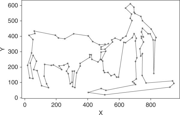
Configural representation of the points in Table 1.

The Curse of Dimensionality

The curse of dimensionality, which refers to the exponential rise in complexity associated with increased dimensionality of maps, is the essential reason why interpretation of multivariate spaces is as difficult as it is. The curse takes many forms (Hastie, Tibshirani, & Friedman, 2001). Consider Figure 3, in which 100 points are distributed across spaces of one, two, and three dimensions. In a single dimension, obviously, they are only .01 units apart. If these points were, for example, personality items, they would provide good “coverage” of the space defined by the single dimension. When the points are distributed in two dimensions, they are .1 units apart, with one point for each of 100 squares making up the two-dimensional space. In general, if k points are uniformly distributed in p-dimensional multidimensional space with a hypervolume of unity, the distance between neighboring points is given by

$$\frac{1}{k^{\frac{1}{p}}}$$ (0.1)

By the time you reach seven dimensions, the distance between neighboring points is more than half the total width of the space. Even in four dimensions, 10,000,000 points would be required to maintain the separation of .01 that was obtained with 100 points in a single dimension. Mentioning the possibility of four dimensions reminds us that the curse of dimensionality is reflected in severe problems of visualization as well. Four dimensions are practically impossible for the human mind to visualize, and as we will see, three dimensions are more difficult than one might think.

Figure 3.

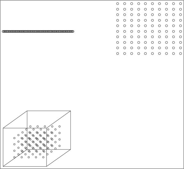
Illustration of the curse of dimensionality in one, two, and three dimensions.

Extensibility to high-dimensional spaces is one advantage of dimensional coordinate systems for representing maps. In terms of simple reproducibility of data, it is no more difficult to represent points in high dimensionality than it is in two, whereas the advantage of graphical systems for understanding configural properties becomes more difficult to realize in three dimensions and evaporates quickly after that. It is important to bear in mind, however, that although dimensional coordinate systems solve certain mathematical aspects of representing complex dimensional spaces, they are not a panacea for the curse of dimensionality. They do not, for example, help with the coverage problem, which is not a problem of reproducibility at all. And the shortcomings of coordinate systems for representing the configural properties of multidimensional spaces are only compounded in high dimensionality.

Multivariate Personality Theory as a Problem in Map Interpretation

This entire section follows closely from Maraun (1997). In the typical multivariate study of individual differences in personality, responses to a set of personality items are obtained from a large sample, usually via self-report. A covariance matrix is computed among the items, which is then submitted to some kind of multivariate statistical procedure such as factor analysis (FA). Describing the process as generally as possible, it can be divided into a sequence of steps:

• Estimation of a similarity or dissimilarity matrix among the items

• Determination of an appropriate reduced dimensionality for this matrix

• Mapping of the location of the items in this reduced space

• Characterization of the mapping using some form of graphical, configural, or coordinate system

• Application of the mapping to obtain multivariate scores for the subjects

Each step in this sequence can be undertaken in many different ways, but a particular set of choices has become dominant in the contemporary personality literature. The similarity matrix is computed as a covariance or correlation matrix among the items; the dimensionality of the space is determined by examination of the eigenvalues of the matrix; factor analysis is used to provide an initial configuration of points in the reduced space; the mapping is characterized dimensionally, using a coordinate system based on rotation to a criterion called simple structure. Small loadings of items on the rotated factors are set to zero, and subject scores are obtained either through formal estimation of factor scores or as unweighted sums of items that load on the rotated factors.

These procedures have become so universally adopted that it is now mostly forgotten that they were once the topic of intense debate among the finest multivariate statisticians of the middle of the twentieth century. A theory of multivariate analysis originating with Louis Guttman offers an alternative route through this sequence of methodological choices. Although the theoretical alternatives proposed by Guttman have been well described by Guttman and his followers and have recently been clearly reiterated in the personality domain (Maraun, 1997), it will be necessary to outline them briefly, especially to establish which differences we think are particularly important.

From the outset, Guttman conceives of the problem more literally in terms of mapping, as opposed to the numerical orientation in terms of matrix decomposition emphasized by factor-analytic approaches. Given a matrix of dissimilarities among a set of items, how can one best locate points in a k-dimensional space so the distance between the points (the distance metric to be employed is another methodological choice that needs to be made) corresponds to the dissimilarity matrix among the items? This problem is familiar to modern researchers as multidimensional scaling (MDS), which is the way we will refer to it here; Guttman's computational procedure was called smallest space analysis.

Guttman's (1955) seminal contribution was to establish that FA and MDS represent alternate paths through the set of methodological choices outlined above and, furthermore, that MDS is the more general of the two. In FA, the similarity matrix is a covariance matrix; in MDS it can be almost any estimate of pairwise difference, including an inverted (to change it from a similarity to a dissimilarity matrix) covariance matrix, a matrix based on some other statistical estimate of distance (such as a rank correlation, or Guttman's underused coefficient of monotonicity, called mu) or human judgments of pairwise differences among stimuli. In FA, items are mapped into space in a way that the angle between their polar coordinates corresponds linearly to their observed similarity; in MDS, items are mapped into space so the Euclidean distance (other distance metrics can be used) between them corresponds to their observed dissimilarity. In the nonmetric variety of MDS favored by Guttman, the correspondence between mapped distance and observed dissimilarity is not constrained to be linear, but merely monotonic.

Although we are convinced by Guttman's argument that the MDS procedures for locating points in reduced dimensional spaces offer many advantages over FA procedures, we also agree with Maraun (1997) that these differences are not at the crux of the matter. At this point in the methodological sequence, FA and MDS have used different methods to accomplish the same thing: Points have been located in a reduced dimensional space in a way that maximizes some criterion of correspondence between the distances among the points and the similarities among the items. From here forward, the problem for either FA or MDS is to characterize the multivariate map that has resulted.

In FA, the near-universal procedure is to select a coordinate system using a criterion called “simple structure” (Thurstone, 1947), which entails finding coordinates that maximize the loadings of the items on one dimension and minimize them on the others, amounting to finding axes that lie as close to the points as possible. Rotation to simple structure has become so commonplace, and the computational methods to conduct it so easy to use, that several important considerations have been widely forgotten. First of all, notwithstanding the simple structure criterion, the location of the coordinate axes through a multivariate space is MBA. From a mathematical point of view, no set of axes is any better than another (Mulaik, 2005; Sternberg, 1977; Thurstone, 1947). The simple structure criterion is a matter of human computational convenience rather than a structural property of the data. One must therefore be very careful about attributing a substantive interpretation to any particular rotation of the coordinate axes. Second, the fit of the data to the simple structure criterion is not a given but is rather an empirical hypothesis about the multivariate map. Many maps, indeed most maps, do not have simple structure. (The mountains in Virginia, for example, lack simple structure in that their location is not conveniently described by a set of coordinate axes.) Personality data in particular have repeatedly been shown to lack simple structure (Church and Burke, 1994; McCrae, Zonderman, Costa, Bond, & Paunonen, 1996). The common practice of setting small loadings to zero after axes have been rotated (or even worse, dropping items that “cross-load” on more than one factor) amounts to imposing simple structure on a map by eliminating the inconvenient parts of the data that fail to fit the model.

The classic example of the failure of dimensional coordinate systems to capture the important structural properties of a psychological phenomenon is Shepard's color perception data (1978), and in this case we refer the reader to Maraun's detailed account. To summarize, Shepard reanalyzed judgments of similarity among 14 color samples, submitted the dissimilarity matrix to an MDS procedure, and found that the resulting configuration of colors formed a circle, a similarity structure called a circumplex by Guttman. The circumplex reveals the structure of similarities among the colors but does not conform to simple structure. Factor analyses of the same data matrix resulted in five orthogonal dimensions that completely missed the essential circumplexical structure of the data.

The Circumplex in Personality Theory

The prominent dimensional system known as the Five-Factor Model (FFM; Goldberg, 1990; McCrae & Costa, 1990) of personality has emerged out of traditional FA (Cattell, 1957). Its development was achieved using the lexical hypothesis, the proposition that individual differences in personality become encoded in the everyday vocabulary. Factor analyses of self- and peer-ascription of adjectival descriptors, many derived from the compilation of Allport and Odbert (1936), resulted in a diversity of factor theories that eventually converged on the FFM outlined by McCrae and Costa (1990). Although the FFM is unquestionably one of the most significant personality research discoveries in recent history, an alternative tradition (Leary, 1957; Kiesler, 1983; Wiggins, 1982) has analyzed a subset of Allport and Odbert's adjectives that were interpersonal in nature and demonstrated that these data exhibited a circumplex structure as well.

Circumplexical models of normal personality have also been applied to the personality disorders (Blashfield, Sprock, Pinkston, & Hodgin, 1985; Pincus & Gurtman, 2006; Soldz, Budman, Demby, & Merry, 1993; Widiger & Hagemoser, 1997; Wiggins & Pincus, 1989). The circumplexical solutions that have been reported have differed in detail but are similar in overall structure. Following Wiggins and colleagues, the circumplex is usually described in terms of octants. Proceeding from the (MBA) top, they are, Dominance, Extraversion, Warmth, Ingenuous, Submissive, Aloof, Cold, and Arrogant (see, e.g., Figure 4.4 in Wiggins, 1996). Several shortcomings of the extant literature will be addressed in the current article. First, all studies reported to date have been based on preexisting PD scale scores rather than on the individual items. Our analysis will show that existing PD scales do not necessarily correspond to the similarity structure of the items.

Figure 4.

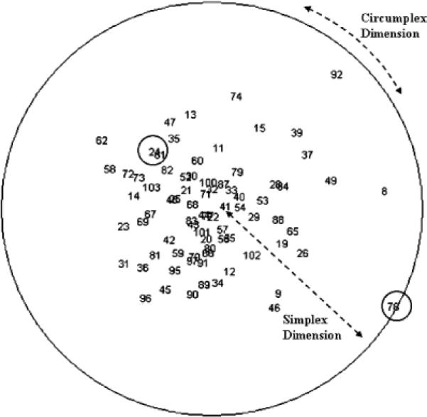
Two-dimensional radex NMDS solution of MAPP PD items.

Second, previous reports have been limited to circumplexical representations in the plane, although many published solutions are obviously not circumplexical. This is particularly true because the solutions often do not form a hollow circle but rather a filled-in disk, which, as we will see, is known as a radex (e.g., Soldz et al., 1993). We find that the radex structure has an important interpretation, and, moreover, that two dimensions are inadequate to represent PD data, leading us to explore solutions in three. Existing circumplexical models that attempt to describe personality data in greater than two dimensions have consisted of multiple orthogonal circumplexes (De Raad & Hofstee, 1993). Although this approach succeeds in demonstrating that the dimensional and circumplexical approaches to multivariate structure are not necessarily at odds with each other, orthogonal circumplexes share many of the disadvantages of orthogonal dimensions for the description of multivariate structure. Returning to our geographic metaphor, describing multivariate space with orthogonal circumplexes is like describing earthly geography only via reference to the “circumplexes” known as the equator and the Greenwich Meridian. Like latitude and longitude applied to two-dimensional maps, spherical coordinates are mathematically sufficient but not necessary and have significant limitations as tools for representing geographical structure.

In summary: (1) Although MDS offers some important advantages over FA as a tool for the representation of complex data in reduced dimensionality, the choice between statistical procedures is not crucial to our case. FA and MDS both represent stimuli in reduced multidimensional space, and the important question is how their configuration in space is to be characterized. (2) Coordinate systems rotated to simple structure are a poor representation of many maps. (3) Even in maps that do show some degree of simple structure, dimensional coordinate systems are not particularly informative about their configural properties. (4) Dimensional coordinates rotated to simple structure, like any concrete system for map characterization, are MBA. This last point is not unique to coordinate systems since the same is true of any alternative that might be proposed. Rather, it contradicts the now-widespread belief that dimensional coordinate systems rotated to simple structure have some special claim on the actual structural properties of the phenomenon under study. They do not.

In the current article we apply regional interpretation of multidimensional scaling analyses to the structure of personality disorder symptoms, using a large sample of self-report data. Although several interesting aspects of the structure of personality disorders are illuminated by a careful interpretation of a two-dimensional model, we find that a three-dimensional model provides a substantially better fit. We then explore some of the considerable difficulties that are encountered in the attempt to perform regional interpretation in three dimensions.

METHOD

Participants

The Multisource Assessment of Personality Pathology (MAPP) was administered to two samples.

Sample 1

This sample consisted of 1562 Air Force recruits (60% male, 40% female) who had just completed basic training at Lackland Air Force Base in San Antonio, Texas. Participants were general enlisted personnel who, upon arrival for 6 weeks of basic training, were grouped together to form units called flights. Unit sizes ranged from 27 to 54 recruits per flight (M = 41, SD = 6.3) and were either same-sex or mixed-sex in composition. The sample comprised 64% Caucasians, 17% African Americans, 9% Hispanics, and 10% other ethnicities (Asian, Native American, or biracial) with ages ranging from 18 to 35 and a mean of 20.2 years (SD = 2.4). Participation in the study was voluntary.

Sample 2

This sample consisted of 1693 college freshmen (33% male, 67% female) attending the University of Virginia. Participants were grouped by the same-sex dormitory hall on which they lived together during the first semester of the academic year. Each group was then assessed during the following spring term. Group sizes ranged from 3 to 21 students (M = 13, SD = 3.4). Participants were 79% Caucasian, 8% Asian, 6% African American, and 7% other ethnicities (Hispanic, Native American, or biracial) with ages ranging from 18 to 27 (M = 18.6, SD = 0.25). For participation, the students received their choice of experiment credit towards a psychology course or monetary compensation.

Measures

Multisource Assessment of Personality Pathology (MAPP)

The MAPP, a personality assessment inventory primarily used as a research instrument in the Peer Nomination Project (Oltmanns & Turkheimer, 2006), consists of 103 items, including 78 that are translations of the DSM-IV (1994) diagnostic criteria for each of the 10 PDs into lay terms (See Table 2). These items were constructed by simplifying the DSM-IV criteria to capture their meaning while eliminating any psychological jargon. One of the criteria for Narcissistic PD, “Is often envious of others or believes that others are envious of him or her (DSM-IV-TR, p. 717),” was split into two separate items: “Is jealous of other people,” and “Thinks other people are jealous of him/her.” Expert consultants in Axis II psychopathology then reviewed the translations and revised them for accuracy and clarity. The remaining 24 items describe positive characteristics, such as “Is sympathetic and kind to others” or “Has a cheerful and optimistic outlook on life.” These were included to decrease the emphasis on pathological personality traits. Only the 78 PD items were used in the current analysis.

Table 2.

Multi-Source Assessment of Personality Pathology PD Items

Item	PD	DSM-IV Criterion
8	SZ	A2
9	ST	A2
11	BD	7
12	NA	2
13	AV	5
14	DP	2
15	OC	2
19	ST	A7
20	AS	A2
21	HS	3
23	NA	4
24	AV	4
25	DP	8
26	OC	8
28	PA	A2
29	SZ	A1
30	ST	A9
31	AS	A3
32	BD	6
33	HS	5
34	NA	9
35	AV	6
36	DP	7
37	OC	7
39	PA	A3
40	SZ	A4
41	ST	A6
42	AS	A6
43	BD	2
44	BD	5
45	HS	6
46	NA	7
47	AV	7
48	DP	6
49	OC	6
52	PA	A4
53	SZ/ST	A5/A8
54	ST	A4
55	AS	A4
56	AS	A7
57	BD	8
58	HS	7
59	NA	8
60	AV	3
61	DP	3
62	OC	5
65	SZ	A7
66	AS	A1
67	BD	1
68	BD	9
69	HS	8
70	NA	5
71	AV	1
72	DP	1
73	DP	4
74	OC	1
77	PA	A6
78	SZ	A6
79	ST	A9
80	AS	A5
81	HS	1
82	AV	2
83	DP	5
84	OC	3
87	PA	A1
88	ST	A3
89	BD	4
90	HS	2
91	NA	1
92	OC	4
95	PA	A7
96	HS	4
97	NA	3
100	ST	A5
101	NA	6
102	PA	A5
103	NA	8

Procedure

As part of a larger study investigating the utility of peer report in personality assessment, participants were screened using a computerized battery of measures. Included in these measures was the self-report portion of the MAPP. Each participant was asked to rate him- or herself on a 4-point scale: (0) Never this way, (1) Sometimes this way, (2) Usually this way, (3) Always this way. Completion of this measure typically ranged from 45 minutes to 1 hour of the total 2 hours of assessment time.

Statistical Procedures

Guttman's Monotonicity Coefficient (Raveh, 1978), μ, was used to estimate the similarities among the 78 PD items of the MAPP. The μ coefficient is a measure of the degree to which the relation between a pair of variables is monotonic, i.e., an increase in the value of one variable is associated with an increase in the value of the other, without assuming linearity of the relation. The magnitudes of these coefficients can range from −1 to 1, where μ = 1 describes a perfect positive monotonic relationship between the two items. Mu was computed using the formula,

$${\mu }_1=\frac{\sum _{i>j}(Y_i-Y_j)}{\sum _{i>j}\mid Y_i-Y_j\mid }1\le j<i\le N$$ (1.2)

where Y_i − Y_j refers to the observed difference between the i^th and j^th items and N is the total number of items in the scale, that is, 78.

The similarity matrix was then submitted to nonmetric multidimensional scaling (NMDS) to recover a spatial representation of the items based on the rank order of the similarities. This analysis was carried out using the SAS System's PROC MDS, which requires the values of the similarities to be positive. To accommodate this constraint, a value of 1 was added to the monotonicity coefficients to shift their values from 0 to 2, where zero describes a perfect “negative” monotonic relationship. Fit of the NMDS solution was assessed with a goodness-of-fit index called Stress Formula 1 (Kruskal & Carroll, 1969).

$$\text{Stress}=\sqrt{\frac{\Sigma {(f\left(x_{ij}\right)-d_{ij})}^2}{\Sigma d_{ij}^2}}$$ (1.3)

In the equation, x_ij are observed pairwise differences, transformed by a monotonic function, f(x_ij); d_ij represents the Euclidean distance between points i and j in the estimated solution. The implication of the monotonic transform f is that only the ordinal properties of the observed distances are being modeled, creating an analysis known as nonmetric multidimensional scaling. Models in which the observed distances are modeled directly are known as metric scaling. Solutions with stress values less than 0.20 were considered to reflect acceptable goodness-of-fit as suggested by Kruskal (1964).

RESULTS

Two-Dimensional Solution

The values of μ ranged from −0.27 to 0.91. Using the transformed μ coefficients as input, NMDS produced stress values of 0.21, 0.15, and 0.12 for the two-, three-, and four-dimensional solutions, respectively, indicating that the three- and four-dimensional solutions fall in the acceptable range. Although the fit in two dimensions was inadequate, this solution was interpreted anyway to provide a basis for the understanding of a subsequent three-dimensional model.

Examination of the overall structure of the configuration revealed that it is best described as a radex, a structure first described by Guttman, 1954 (Figure 4). It may be that the failure of Guttman-style interpretation of multivariate spaces can be attributed to the superficially unimpressive appearance of a radex, which looks suspiciously like a scatterplot of the relation between two variables that have turned out to be uncorrelated. In fact, the radex is highly structured. It consists of two components—a circular dimension called a circumplex and an inner-outer dimension running from the center of the configuration to the perimeter, called a simplex.

To follow our interpretation of the solution that follows, it will be important to understand the details of the mapping of the radex structure onto the pairwise item similarities. Recall that the NMDS solution is a literal representation of inter-item similarity. Around the periphery of the solution, items are close to those around them but far away from equally peripheral items on the other side of the configuration. For example, Item 24 is estimated to be very similar to Item 61 but quite dissimilar to Item 78. In contrast, items near the center of the configuration are estimated to be roughly equal in similarity to items around the perimeter of the circumplex. These items, therefore, are more globally typical of the entire domain, rather than being specific to a particular region. To illustrate this property, we computed the corrected item-total correlations (the correlation of each item with the total of the other items) and plotted them against the distance between the modeled location of each item and the center of the solution. The result is shown in Figure 5. The core items are more broadly representative of the overall tendency to self-report Axis-II symptoms.

Figure 5.

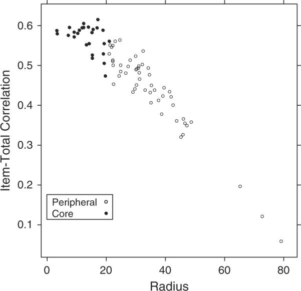
Item-total correlation as a function of item radius. Vertical line separates “core” items from “peripheral” items.

The radex produced by the two-dimensional solution was given a preliminary interpretation using a neighborhood or regionalization approach (Guttman, 1965) in which the content of adjacent items were examined to identify areas of similar content that could be grouped together to form MBA regions. These regions included seven positioned radially around the circumplex and a central region we refer to as the core (See Figure 6). We emphasize that the regions are strictly MBA, drawn only to help the human eye understand the regional structure of the mapping. Note also that we specifically avoid the practice, common even in MDS applications, of selecting arbitrary dimensions through the space for interpretation. Although such lines would be no more arbitrary than the regional boundaries we have drawn, habits of mind are such that most readers would quickly begin to reify them if they were included.

Figure 6.

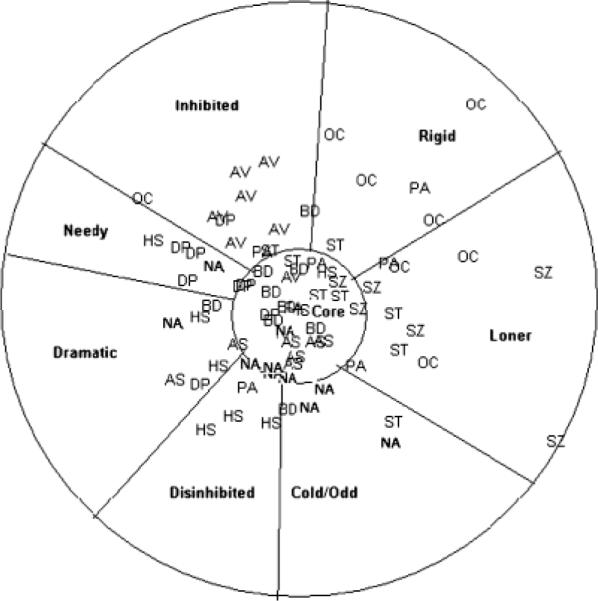
MBA regionalized two-dimensional NMDS solution of the MAPP PD items.

The core region, because of its central location in the radex, contains items that are generally similar to all of the surrounding regions, as opposed to being characteristic of any one of them. It consisted of criteria from 9 of the 10 DSM-IV (2000) PDs. Borderline PD (BPD) and Antisocial PD (ASPD) items were the most prevalent in the core (see Table 3). Although BPD and ASPD shared equal representation in the core with regard to number of criteria, it should be remembered once again that our demarcation of the boundary around the core region was MBA. To assess which diagnostic category was most representative of the center of the radex, we computed the radius of each item, or the Euclidean distance of each item to the center of the configuration. BPD items were closest to the center, followed by Schizotypal and Antisocial (Table 4). The criteria for obsessive-compulsive PD were the furthest from the center of the configuration, suggesting that the OC criteria are the least characteristic of the overall domain of Axis II criteria. We will interpret the structure of the regions in more detail as we proceed to the three-dimensional solution.

Table 3.

Regions of Two-Dimensional Solution

	Number of DSM-IV Criteria
Region	BD	AS	ST	HS	PA	NA	DP	AV	SZ	OC
Core	5	5	3	2	2	2	1	1	1	0
Rigid	0	0	1	0	1	0	0	0	0	4
Loner	0	0	1	0	2	0	0	0	6	3
Cold/Odd	1	0	1	0	0	4	0	0	0	0
Disinhibited	0	0	0	3	1	2	0	0	0	0
Dramatic	1	2	0	2	0	1	1	0	0	0
Needy	0	0	0	1	0	3	3	0	0	1
Inhibited	1	0	1	0	0	0	1	6	0	0

Table 4.

Mean Distance of PDs From Center of Two-Dimensional Solution

PD	Mean Radius
Borderline	14.79
Schizotypal	18.93
Antisocial	19.08
Paranoid	22.42
Dependent	25.27
Narcissistic	26.19
Avoidant	28.64
Histrionic	28.79
Schizoid	36.55
Obsessive-compulsive	46.37

To compare the NMDS solution to a traditional simple structure solution derived from factor analysis, an exploratory factor analysis of the 78 MAPP items was performed using M Plus. The number of factors needed to represent the MAPP was determined using the Kaiser-Guttman criterion of considering factors that have eigenvalues greater than 1.0 and by considering factor interpretability. Model fit was gauged by the Root Mean Square Error of Approximation (RMSEA) statistic where an RMSEA less than 0.05 is considered acceptable (Browne & Cudeck, 1993). Using these considerations a five factor solution was accepted as showing both good model fit (RMSEA=0.03) and interpretability.

Interpretation of the factor loadings was conducted following a Promax rotation of the original factor solution. The correlations among the factors in this analysis were found to be small to moderate, ranging from 0.23 to 0.49 (see Table 5). A loading cut of .30 was used for inclusion of an item in interpretation of a factor; consequentially 6 of the 78 items failed to be included in any of the five factors as seen in Table 6. Inspection of the content of the items with the highest loadings on each of the factors resulted in the following labels: Unrestrained, Dependent, Reckless, Rigid/Loner, and Identity Problems.

Table 5.

Correlations Among the Five Promax Rotated Factors

Factor	Unrestrained	Dependent	Reckless	Rigid/Loner	ID Problems
Unrestrained	–
Dependent	0.41	–
Reckless	0.40	0.30	–
Rigid/Loner	0.30	0.30	0.23	–
ID Problems	0.49	0.43	0.41	0.40	–

Table 6.

Loadings of a Five Factor Solution of the MAPP

	Factors
Item	Unrestrained	Dependent	Reckless	Rigid/Loner	ID Problems	h2
8	−0.06	−0.23	−0.10	0.48	0.25	0.36
9	0.09	0.05	0.05	−0.04	0.39	0.17
11	−0.20	0.27	0.01	0.12	0.59	0.48
12	0.41	0.03	0.02	0.09	0.23	0.23
13	−0.25	0.54	−0.05	0.22	0.25	0.47
14	0.05	0.51	0.20	−0.11	0.15	0.34
15	0.04	0.15	0.19	0.21	0.06	0.11
19	−0.07	−0.04	0.22	0.03	0.57	0.38
20	0.34	−0.02	0.31	−0.02	0.34	0.33
21	−0.03	0.35	0.14	−0.02	0.48	0.37
22	0.10	0.11	0.24	0.07	0.44	0.28
23	0.61	0.33	−0.19	−0.14	0.14	0.56
24	0.14	0.72	−0.27	0.00	0.24	0.67
25	0.04	0.55	0.29	−0.02	0.14	0.41
26	0.26	−0.12	−0.04	0.22	0.33	0.24
28	0.00	−0.02	0.07	0.39	0.38	0.30
29	−0.03	−0.03	0.39	0.39	0.23	0.36
30	0.12	0.41	−0.08	0.13	0.38	0.35
31	0.10	0.07	0.30	−0.27	0.42	0.35
32	0.01	0.18	0.04	0.03	0.62	0.42
33	−0.13	0.20	0.31	0.10	0.41	0.33
34	0.64	−0.05	0.08	0.14	−0.01	0.44
35	−0.12	0.55	−0.14	0.06	0.41	0.51
36	0.29	0.13	0.33	−0.10	0.07	0.22
37	0.18	0.11	0.05	0.26	0.02	0.12
39	−0.05	0.09	0.08	0.43	0.09	0.21
40	−0.15	0.15	0.39	0.33	0.24	0.36
41	−0.07	0.13	0.28	0.12	0.52	0.39
42	0.11	0.16	0.48	−0.12	0.21	0.33
43	0.27	0.14	0.26	0.02	0.32	0.26
44	0.11	0.23	0.54	0.15	0.19	0.42
45	0.56	−0.01	0.11	−0.12	0.15	0.36
46	0.17	−0.14	0.46	0.27	0.05	0.21
47	−0.08	0.60	−0.01	0.25	0.00	0.43
48	0.00	0.60	0.40	0.03	−0.01	0.52
49	0.26	0.00	−0.20	0.44	0.10	0.31
52	0.19	0.35	−0.09	0.10	0.39	0.33
53	−0.12	0.02	0.39	0.50	0.13	0.43
54	−0.08	0.13	0.30	0.12	0.44	0.32
55	0.25	−0.09	0.28	0.14	0.35	0.29
56	0.24	−0.07	0.48	0.23	0.11	0.36
57	0.19	−0.06	0.35	0.17	0.36	0.32
58	0.10	0.65	0.04	−0.10	−0.01	0.44
59	0.67	0.08	0.17	0.08	−0.10	0.50
60	−0.03	0.51	0.11	0.33	0.06	0.39
61	0.02	0.69	0.04	0.11	0.01	0.49
62	0.11	0.33	−0.02	−0.03	0.14	0.14
65	0.02	−0.22	0.35	0.48	0.19	0.44
66	0.28	−0.11	0.62	0.03	0.08	0.48
67	0.09	0.47	0.46	−0.02	−0.10	0.45
68	0.13	0.27	0.14	0.01	0.42	0.29
69	0.23	0.29	0.22	0.04	0.06	0.20
70	0.59	0.05	0.28	0.16	−0.13	0.47
71	0.04	0.37	0.27	0.32	0.08	0.32
72	0.08	0.61	0.13	−0.05	0.01	0.40
73	0.02	0.69	0.25	−0.03	−0.08	0.55
74	0.13	0.31	−0.07	0.45	−0.18	0.35
77	0.27	0.14	0.18	0.21	0.24	0.23
78	0.05	− 0.34	0.16	0.21	0.04	0.19
79	−0.08	0.24	0.18	0.42	0.21	0.32
80	0.26	−0.06	0.54	0.03	0.19	0.40
81	0.65	0.12	0.07	−0.06	0.04	0.45
82	0.18	0.51	0.03	0.15	0.06	0.32
83	0.22	0.32	0.53	0.09	−0.05	0.44
84	−0.01	0.10	0.30	0.54	−0.09	0.40
87	0.08	0.22	0.13	0.35	0.23	0.25
88	0.01	0.00	0.18	0.18	0.42	0.24
89	0.26	−0.16	0.52	−0.12	0.27	0.45
90	0.41	−0.09	0.46	−0.07	0.02	0.39
91	0.68	−0.05	0.25	0.15	−0.10	0.56
92	0.12	0.07	−0.10	0.37	−0.21	0.21
95	0.20	0.07	0.34	0.08	0.09	0.18
96	0.70	0.04	0.06	−0.08	−0.09	0.51
97	0.63	0.04	0.29	0.13	−0.17	0.53
100	0.06	0.33	0.07	0.23	0.33	0.28
101	0.37	0.08	0.47	0.11	0.05	0.38
102	0.27	0.10	0.03	0.16	0.24	0.17
103	0.37	0.49	−0.12	0.00	0.15	0.41

Based on the factor-analytic solution, the items composing each factor were located in the NMDS derived space. Upon visual inspection, the items associated with a given factor were found to group together in a reasonably contiguous manner as illustrated in Figure 7. The factor-based regions are simply another MBA regionalization of the two-dimensional NMDS space, reasonable enough on its own terms, but with no special claim to the “true” multivariate structure of the data.

Figure 7.

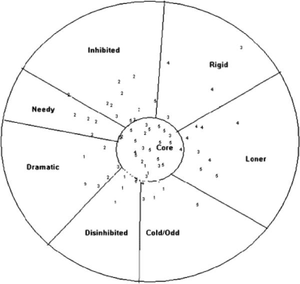
Two-dimensional NMDS solution. Numbers correspond to factors from Promax rotation of FA with five factors: 1 = Unrestrained, 2 = Dependent, 3 = Reckless, 4 = Rigid/Loner, 5 = ID Problems.

To quantify the amount of information lost by discarding items with factor loadings that did not meet the 0.3 cutoff we performed an analysis proposed by Maraun (1997). Maraun pointed out that since all of the factor loadings are required to represent the configuration of the items, removing loadings in order to impose very simple structure results in a loss of information. To quantify this loss, which Maraun called the percentage of structure ignored, the sums of squares of the factor loadings less than the cut score are divided by the total sum of squares of all factor loadings. Application of this method to our FA result showed that 23% of the structure was ignored by choosing only to interpret factor loadings greater than the cutoff.

Three-Dimensional Solution

As we have already noted, the two-dimensional NMDS model does not meet conventional fit criteria. We suspect that this is not an uncommon outcome, and the difficulties we encounter in the regional interpretation of the three-dimensional solution may suggest why most MDS analyses of personality data stop at two dimensions despite marginal fit. Modern computer graphics offer many advantages in the visualization of three-dimensional data, and we think we achieve some success in what follows, although in a journal format we are also hamstrung by the constraints of static grayscale images.

We began our interpretation of the three-dimensional NMDS by comparing it to the two-dimensional result. To facilitate comparison, a procrustes rotation was applied to the coordinates produced by the three-dimensional solution, with a criterion of rotating the first two dimensions of the 3-D solution to conform as closely as possible to the two-dimensional solution, with the third dimension orthogonal to the first two (see Figure 8). Aligning the solution in this manner emphasizes the additional information that is provided by the third dimension. Despite the attempt to make the relationship between the two- and three-dimensional solutions more apparent, however, the problem of regionalization, which was a matter of straightforward intuition in two dimensions, becomes much more difficult in three. The task is now to divide three-dimensional space into “chunks” that regionalize space in the same way that outlined areas regionalize the plane. The eye has a hard time following and making sense of the spatial relationships among the items once they are arrayed in three dimensions.

Figure 8.

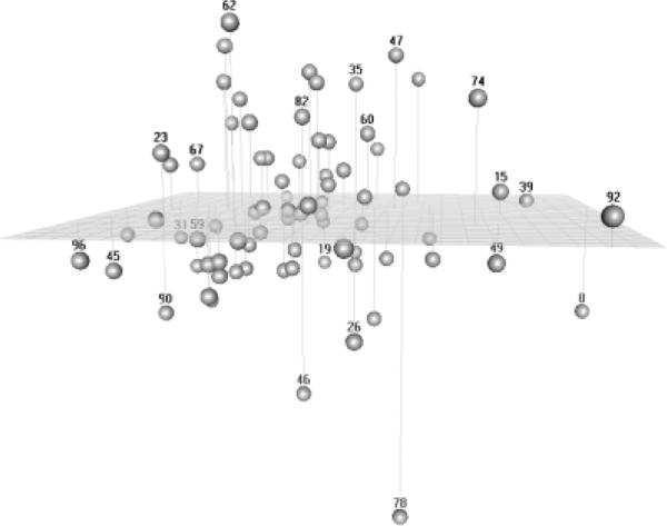
Procrustes rotated three-dimensional NMDS solution. First two dimensions correspond as closely as possible to two-dimensional solution, with new third dimension orthogonal.

In order to solve this problem in multidimensional data visualization, we relied on our knowledge of the structure of the similarity space in two dimensions: a core region containing items that were moderately similar to all other items, surrounded by a circumplex of items that were highly similar to their neighbors but different from those on the other side of the circumplex. With this in mind, we simplified the three-dimensional configuration into two structures, a core and a spherex. The core region was specified using the third of the items that were closest to the centroid of the three-dimensional configuration. The coordinates of the remaining items were projected to the surface of a unit sphere (see Figure 9).

Figure 9.

Regionalized MAPP PD items on the surface of the sphere.

We then attempted to characterize the regional structure of the core and the spherex. The relatively smaller number of items in the core could be regionalized in terms of four three-dimensional regions: Suspiciousness, Anger, Isolation, and Identity problems. This core configuration is illustrated in Figure 10. Once the noncore items have been projected outward to the spherex, the problem becomes one of identifying MBA regions on the surface of a globe. The item content of adjacent items on the sphere was examined for similarity and separated as before to form eight regions as illustrated in Figure 9. These regions are very similar to those defined in the two-dimensional solution except for the emergence of a Schizotypy region at the northern polar cap (with MBA orientation!) of the sphere.

Figure 10.

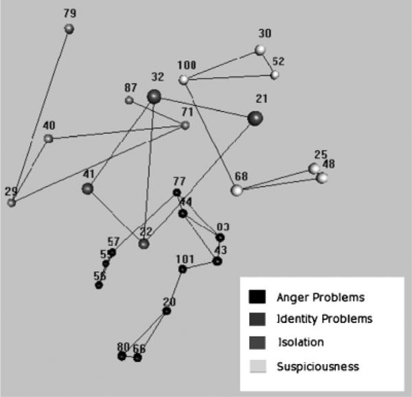
MBA structure of core the three-dimensional NMDS solution. Lines are drawn to help visualize four three dimensional regions of core: suspiciousness, aggressiveness, isolation, and identity disturbance.

DISCUSSION

When stimuli of high dimensionality are submitted to a multivariate statistical procedure that maps them into a lower dimensionality, characteristics of the data fix two aspects of the result—its dimensionality and its structure. Although, in our view, applied data generally do not have a “true” dimensionality that can be ascertained by the researcher, the fit of a model in any given reduced dimensionality is, nevertheless, strictly a characteristic of the data themselves. By the “structure” of the data we refer to their shape or configuration in the multidimensional space that is chosen. Once again, applied data are unlikely to result in a perfectly circular configuration, and it is up to the researcher to decide whether a given configuration is close enough to a perfect circumplex to ignore the differences. The shape of the locations of the items in the reduced space, however, is determined by the multivariate structure of the data.

All subsequent interpretations of multivariate results are MBA. The data do not militate which end of a configuration belongs on top, leaving the investigator free to orient the configuration as he or she wishes. This freedom can be a boon to flexible and descriptive interpretation of multivariate data, but it comes with the inherent danger that the investigator will soon forget that the decision to orient the data in a particular way was a matter of convenience, not empirical fact. Such a misguided investigator might then begin to assign empirical meaning to these orientations, like a child who wonders whether the location of the northern hemisphere on top of the globe is a reflection of some inherent superiority over the south.

Our admittedly oversimplified account of Guttman's scientific prescription is that multivariate science should be focused resolutely on quantification of dimensionality and interpretation of configural structure because this is where empirical constraints on our theorizing are located. The data determine how many dimensions are required to represent self-reported PD symptoms at some criterion of accuracy, and within that mapping the data determine the contiguity of like to like and the configuration of the structure of the whole. Although some form of line drawing is necessary to make sense of a multidimensional mapping, all line drawing is MBA. We prefer drawing of regions to the more common drawing of dimensions for several reasons. First, it serves as a corrective to the prevailing habit of believing that dimensions defined by simple structure are a reflection of natural laws; for whatever reason, scientists appear to be more willing to accept regions for what they are, that is, as meaningful but arbitrary contingencies in the service of multidimensional description. Second, regions are a more flexible method for operationalizing the crucial concept of contiguity as a means of capturing the location of the mountains in Virginia or the narcissism items in a mapping of the MAPP. Straight lines extending from positive to negative infinity are very limiting as a means of categorizing spatial configurations of contiguity, especially as regards soft psychological data.

Our regional investigation of the structure of the MAPP has demonstrated several interesting facts about the structure of the personality disorders. The circumplexical aspect of our solution is generally similar to Wiggins's version of the interpersonal circle (1995). To provide some orientation between the two representations, the Disinhibited region in our two-dimensional model can be viewed as a blending between the vindictive and domineering octants of the IPC. Both describe the portion of personality space made of narcissistic and domineering traits. Once the two models are aligned in this way, one can continue about the circle and find fairly direct correspondence between them based on their regional content. Minor differences are likely to be attributable to our use of individual criteria rather than predefined scales, as our analysis shows that scales do not correspond very well to the actual locations of the items.

Soldz et al. (1993) reported a solution that looked more like a radex than a circumplex, but they did not offer an interpretation of the radexical dimension. They also reported the “surprising” conclusion that Borderline PD was located close to the origin. We have shown that the radex dimension of the solution has a clear interpretation that has important implications for our understanding of personality disorders: certain traits, which we have characterized as anger, isolation, suspiciousness, and identity disturbance, are common to all of the PDs in the concrete sense that they have high item-total correlations with the universe of PD symptoms. Other traits, which can be viewed as more specialized variants of the core traits, are typical of specific types of PD but not of the universe as a whole. From Table 7, one can see that the mu coefficients of core regions with each of the 10 PD scales of the MAPP are generally higher compared to the regions located on the spherex. This relationship is perhaps more apparent when examining the spread and the median of each region's similarity to the 10 PDs in Figure 11.

Table 7.

Similarities of the Three-Dimensional Regions to the 10 DSM-IV PDs

Region	BD	AS	ST	HS	PA	NA	DP	AV	SZ	OC
Anger Problems	0.96	0.98	0.90	0.90	0.90	0.92	0.86	0.76	0.80	0.72
Identity Problems	0.97	0.83	0.91	0.86	0.84	0.78	0.82	0.80	0.74	0.67
Isolation	0.88	0.81	0.93	0.78	0.93	0.78	0.81	0.85	0.87	0.75
Suspiciousness	0.94	0.81	0.93	0.86	0.91	0.84	0.94	0.89	0.64	0.74
Rigid	0.73	0.55	0.74	0.63	0.79	0.65	0.67	0.71	0.67	0.95
Loner	0.73	0.67	0.87	0.59	0.84	0.68	0.54	0.63	0.93	0.84
Cold/Odd	0.75	0.77	0.75	0.69	0.78	0.85	0.57	0.52	0.82	0.73
Disinhibited	0.84	0.88	0.76	0.96	0.79	0.96	0.76	0.59	0.62	0.65
Dramatic	0.89	0.92	0.79	0.95	0.76	0.91	0.90	0.75	0.55	0.64
Needy	0.83	0.71	0.73	0.84	0.73	0.78	0.96	0.86	0.38	0.73
Inhibited	0.81	0.64	0.79	0.73	0.77	0.72	0.89	1.00	0.50	0.68
Schizotypy	0.85	0.78	0.98	0.79	0.74	0.70	0.70	0.68	0.80	0.62

Figure 11.

Each three-dimensional region's similarity to the 10 DSM-IV PDs.

The radex, we think, provides a ready explanation for the most commonly expressed shortcoming of Axis II, the high level of comorbidity among the PD subtypes. According to our account, PD subtypes overlap for two essential reasons. First of all, it is in the nature of regional descriptions of maps that neighboring regions will sometimes overlap in practice. Is Missouri a midwestern state or a southern one? Numeric dimensional systems for mapping solve the problem of overlap at the expense of rich configural description of the space. The second reason for comorbidity, one more specifically related to the empirical properties of PD criteria we have described, is because the various diagnostic entities share traits that are common to the entire domain. An individual who is withdrawn, hostile, and suspicious, with changeable identity, is at risk for practically any personality disorder, and it is no surprise that many such people qualify for several of them. Figure 12 is a schematic representation of how common traits might lead to comorbidity among the PDs.

Figure 12.

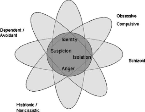
Schematic representation of trait comorbidity, illustrating that regional PD diagnoses can be expected to overlap because they share common core traits.

Another longstanding, if less frequently addressed, issue involves the special standing of Borderline PD among the personality disorders. Borderline was among the first PDs to be recognized clinically and retains an iconic status among personality disorders. Why? In fact, conventional psychometric and factor-analytic studies of the PDs suggest that the two main characteristics of Borderline PD, emotional dysregulation and identity disturbance, do not seem to belong together in the same syndrome (Thomas, Turkheimer, & Oltmanns, 2003). These conventional analyses, however, lack the radexical concept of core traits that we have developed here. Of all the PDs, BD symptoms lie closer to the core of the domain by a considerable margin. Borderline PD is literally iconic: It comprises the traits that define the universe of PDs.

It is also important to emphasize that many other MBA regionalizations of the PD domain are possible and interesting, and indeed might be desirable under some circumstances. For example, in Figure 6 the location of the narcissism items have been printed in boldface. Although their location does not correspond very well to the regionalization we have chosen, they nevertheless form a nearly contiguous region of the space, and characterizing that region helps us to understand the relation of narcissistic traits to other PD traits. Narcissism is a trait that is moderately typical of PDs in general, running along an axis from a needy concern with social standing (“is jealous of others,” “needs to be admired”) to an aloof disdain for others (“is not concerned for other people's feelings or needs”). The mutual proximity of the narcissism criteria suggests that it would be a reasonably good trait if we chose to use it (coefficient alpha for the 10 narcissism criteria, including the 2 items for the single jealousy criterion, is 0.82). If, on the other hand, we prefer the circumplexical regionalization as described in this article, the narcissistic concern with social standing will be treated separately from the aloofness. Both characterizations are valid and MBA.

Although it does not change the methodological framework presented in this article, we chose self-report in the current study as the basis of our analysis in the interest of consistency with the traditional literature on assessment of PD traits. We recognize that clinical experience and empirical evidence suggests that self-report of personality characteristics has its shortcomings, and indeed those who are familiar with the Peer Nomination Project are aware that peer report data was collected to supplement the self-report data we have used here (Klonsky, Oltmanns, & Turkheimer, 2002). We intend to conduct similar analyses in the peer nomination data and compare the degree to which the solution remains invariant.

CONCLUSION

The early factor analysts faced a difficult theoretical problem. They had established a goal of using factor analysis as a tool for uncovering the underlying causal mechanisms of mind and behavior in a domain where randomized experimentation was usually impossible. It turned out, however, that the structures discovered by factor analysis were indeterminate in several important senses. How can factor-analytic solutions correspond to causal biological processes if an infinite number of solutions fit equally well? The concept of simple structure was Thurstone's answer to this conceptual dilemma. Among all possible solutions, Thurstone presumed that the one with the greatest parsimony would correspond to physical reality, and he invested much of his genius in the enterprise of demonstrating that the property of simple structure remained lawfully invariant across behavioral and psychometric domains.

To the extent Thurstone's hypothesis is correct in any particular domain and the dimensions identified by simple structure do indeed capture the essential causal underpinnings of complex multivariate systems the process of detailed configural description of multivariate space as we have described it here becomes relatively unnecessary. If one is convinced that a small set of orthogonal dimensions provides a compelling scientific account of a multivariate domain, then measurement of persons on those dimensions are all that is required. Assessment, as opposed to mere measurement, with its connotation of configural description of the multivariate topography, is unnecessary (Matarazzo, 1990). If, however, the structure of a multivariate-item space (a) consists of more than a single dimension and (b) lacks simple structure in the sense that informative items are distributed throughout the multidimensional space, then the configuration of an individual's pattern of responses in the space will be poorly characterized by a set of means on arbitrary orthogonal dimensions. Descriptive characterization of an individual's tendency to endorse items in an MBA narcissistic region of the space requires a structural system that is more flexible than a fixed set of dimensions or diagnostic categories. The discovery and description of such regions is what is connoted by the term assessment over and above the more straightforward measurement.

From the earliest beginnings of the factor-analytic enterprise, some have harbored the suspicion that the dimensions derived by factor analysis and specified in terms of simple structure do not always represent causal reality. Perhaps they are simply mathematical conveniences, fit post hoc to covariance structures that were determined by other processes entirely. The great British factor analyst Godfrey Thomson, quoted by Thurstone himself,¹ expressed his skepticism as follows:

Briefly, my attitude is that I do not believe in `factors' if any degree of real existence is attributed to them; but that of course I recognize that any set of correlated human abilities can always be described mathematically by a number of uncorrelated variables or “factors,” and that in many ways…. My own belief is that the mind is not divided up into “unitary factors,” but is a rich, comparatively undifferentiated complex of innumerable influence (p. 267).

What is left for the personologist who no longer believes in the scientific reality of simple structure? It may seem too much to ask the scientist who has envisioned a systematic, replicable causal account of a psychological system to settle instead for detailed description and assessment of the structure of the multivariate phenomena at hand, but that is what is available to nonexperimental multivariate scientists. And as Guttman recognized, modern statistical and computational methods could be extraordinarily rich sources of multivariate scientific description if only we would let them. A revival of Guttman's insight is long overdue in the field of personality and its disorders.

REFERENCES

- Allport GW, Odbert HS. Trait names: A psycholexical study. Psychological Monographs. 1936;47:211. [Google Scholar]
- American Psychiatric Association . Diagnostic and statistical manual of mental disorders: DSM-IV. Author; Washington, DC: 1994. [Google Scholar]
- Blashfield RK, Sprock J, Pinkston K, Hodgin J. Exemplar prototypes of personality disorder diagnoses. Comprehensive Psychiatry. 1985;26:11–21. doi: 10.1016/0010-440x(85)90045-8. [DOI] [PubMed] [Google Scholar]
- Browne MW, Cudeck R. Alternative ways of assessing model fit. In: Bollen K, Long S, editors. Testing structural equation models. Sage; Newbury Park, NJ: 1993. pp. 136–162. [Google Scholar]
- Cattell Raymond B. Personality and motivation structure and measurement. World Book Co; 1957. [Google Scholar]
- Church AT, Burke PJ. Exploratory and confirmatory tests of the Big Five and Tellegen's three- and four-dimensional models. Journal of Personality and Social Psychology. 1994;66:93–114. doi: 10.1037//0022-3514.66.1.93. [DOI] [PubMed] [Google Scholar]
- De Raad B, Hofstee WKB. A circumplex approach to the trait adjectives supplemented by trait verbs. Personality and Individual Differences. 1993;15:493–505. [Google Scholar]
- Freud S. New introductory lectures on psychoanalysis. Norton; New York: 1965/1933. [Google Scholar]
- Goldberg LR. An alternative “description of personality”: The Big-Five factor structure. Journal of Personality and Social Psychology. 1990;59:1216–1229. doi: 10.1037//0022-3514.59.6.1216. [DOI] [PubMed] [Google Scholar]
- Guttman . A new approach to factor analysis: The radex. In: Lazarsfeld PS, editor. Mathematical thinking in the social sciences. Free Press; New York: 1954. [Google Scholar]
- Guttman L. A generalized simplex for factor analysis. Psychometrika. 1955;20:173–192. [Google Scholar]
- Guttman The structure of intercorrelations among intelligence tests; Proceedings of the 1964 Invitational Conference on Testing Problems; Princeton, NJ: Educational Testing Service; 1965. [Google Scholar]
- Hastie T, Tibshirani R, Friedman J. The elements of statistical learning. Springer; New York: 2001. [Google Scholar]
- Kiesler DJ. The 1982 interpersonal circle: A taxonomy for complementarity in human transactions. Psychological Review. 1983;90:185–214. [Google Scholar]
- Klonsky ED, Oltmanns TF, Turkheimer E. Informant reports of personality disorder: Relation to self-reports and future research directions. Clinical Psychology: Science and Practice. 2002;9:300–311. [Google Scholar]
- Kruskal JB. Multidimensional scaling by optimizing goodness of fit to a non-metric hypothesis. Psychometrika. 1964;29:1–27. [Google Scholar]
- Kruskal JB, Carroll JD. Geometric models and badness of fit functions. In: Krishnaiah PR, editor. Multivariate analysis. Academic Press; New York: 1969. pp. 639–671. [Google Scholar]
- Leary T. Interpersonal diagnosis of personality. Ronald; New York: 1957. [Google Scholar]
- Maraun MD. Appearance and reality: Is the big five the structure of trait descriptors? Personality and Individual Differences. 1997;22:629–647. [Google Scholar]
- Matarazzo JD. Psychological assessment versus psychological testing: Validation from Binet to the school, clinic, and courtroom. American Psychologist. 1990;45:999–1017. doi: 10.1037//0003-066x.45.9.999. [DOI] [PubMed] [Google Scholar]
- McCrae RR, Costa PT., Jr. Personality in adulthood. Guilford; New York: 1990. [Google Scholar]
- McCrae R, Zonderman A, Costa P, Bond M, Paunonen S. Evaluating replicability of factors in the Revised NEO Personality Inventory: Confirmatory factor analysis versus procrustes rotation. Journal of Personality and Social Psychology. 1996;70:552–566. [Google Scholar]
- Mulaik Stanley A. Looking back on the indeterminacy controversies in factor analysis. In: Maydeu-Olivares A, McArdle JJ, editors. Contemporary psychometrics: A festschrift for Roderick P. McDonald. Erlbaum; Mahwah, NJ: 2005. pp. 173–206. [Google Scholar]
- Oltmanns TF, Turkheimer E. Perceptions of self and others regarding pathological personality traits. In: Krueger RF, Tackett JL, editors. Personality and psychopathology. Guilford; New York: 2006. pp. 71–111. [Google Scholar]
- Pincus AL, Gurtman MB. Interpersonal theory and the interpersonal circumplex: Evolving perspectives on normal and abnormal personality. In: Strack S, editor. Differentiating normal and abnormal personality. 2nd ed. Springer; New York: 2006. pp. 83–111. [Google Scholar]
- Raveh A. Guttman's regression-free coefficients of monotonicity. In: Shye S, editor. Theory construction and data analysis in the behavioral sciences. Jossey-Bass; San Francisco: 1978. [Google Scholar]
- Shepard R. The circumplex and related topological manifolds. In: Shye S, editor. Theory, construction and data analysis in the behavioral sciences. Jossey-Bass; San Francisco: 1978. [Google Scholar]
- Soldz S, Budman SH, Demby A, Merry J. Representation of personality disorders in circumplex and five-factor space: Explorations with a clinical sample. Psychological Assessment. 1993;5:41–52. [Google Scholar]
- Sternberg RJ. Intelligence, information processing, and analogical reasoning. Erlbaum; Hillsdale, NJ: 1977. [Google Scholar]
- Thomas C, Turkheimer E, Oltmanns TF. Factorial structure of personality as evaluated by peers. Journal of Abnormal Psychology. 2003;112:81–91. [PMC free article] [PubMed] [Google Scholar]
- Thurstone LL. Multiple-factor analysis. University of Chicago Press; Chicago: 1947. [Google Scholar]
- Widiger TA, Hagemoser S. Personality disorders and the interpersonal circumplex. In: Plutchik R, Conte HR, editors. Circumplex models of personality and emotions. American Psychological Association; Washington, DC: 1997. pp. 299–325. [Google Scholar]
- Wiggins JS. Circumplex models of interpersonal behavior in clinical psychology. In: Kendall PD, Butcher JN, editors. Handbook of research methods in clinical psychology. Wiley; New York: 1982. [Google Scholar]
- Wiggins JS. The five-factor model of personality. Guilford; New York: 1996. [Google Scholar]
- Wiggins JS, Pincus AL. Conceptions of personality disorders and dimensions of personality. Psychological Assessment: A Journal of Consulting and Clinical Psychology. 1989;1:305–316.s. [Google Scholar]