Interstitial Adenosine: The Measurement, The Interpretation

In the current issue, Gidday et al. report on their observations in “Heterogeneity and Sampling Volume Dependence of Epicardial Adenosine Concentrations.”

I read their report with some anticipation. Was this the long awaited critical assessment of the epicardial disc technique for obtaining estimates of interstitial adenosine concentrations? The other promise was in the word “heterogeneity,” which stimulated my long standing (Yipintsoi et al., 1973) interest in figuring out why the range of normal myocardial blood flows is so broad, at all levels of spatial resolution (Bassingthwaighte, King and Roger, 1989). Could local adenosine concentrations be the governor, as proposed originally by the senior author, Robert Berne (1963)?

The two aspects of the title, the heterogeneity of interstitial fluid (ISF) adenosine concentrations, [Ado]_isf, and the accuracy and reproducibility of methods for estimating [Ado]_isf, are linked: the methods need to be well worked out in order to contemplate the physiology. All currently available methods for estimating [ADO]_isf are indirect. There are various ways of collecting “sweat” or transudate from the epicardial surface, using a small well (Hanley et al., 1983), or epicardial drippings (Decking et al., 1988; Heller and Mohrman, 1988; Mohrman and Heller, 1990). Placing absorbent discs on the epicardium gives estimates similar to the transudates (Tietjan et al., 1990; Headrick et al., 1991). Gidday et al. (1991) report average values of about 470 nm, using discs.

Transudates and disc fluids have the disadvantage, for interpretation, of representing mainly or only the subepicardial interstitium. Methods for estimating the whole heart average myocardial interstitial adenosine from measures of flows, from membrane and capillary wall permeabilities, from volumes of distribution, and from the venous outflow adenosine concentrations (Bassingthwaighte et al., 1985; Wangler et al., 1989; Gorman et al., 1991) are also indirect, but do attempt to take into account the known and measurable flow heterogeneities.

The applications of these methods give widely disparate estimates of interstitial adenosine levels, as reviewed in Table 1, taken from Gorman et al. (1991). No two methods have been applied simultaneously to one heart. What is more awkward is that the most direct measures are local and the global measures can only give an average.

TABLE 1.

Estimates of [ADO]_isf in isolated guinea-pig hearts

Method	Conditions	[ADO]v nM	[ADO]isf nM	ISF/Venous Ratio	Predicted [ADO]isf, nM	Reference
Transudate	Rest	30	180	6	73	Decking (1988)
Transudate	Rest	37	191	5	113	Mohrman (1990)
	Dipyridamole	90	785	9	623
SAH	Rest	9	80‡	9	13	Deussen (1988)
Epicardial disk	Rest	4	280	70	6	Tietjan (1990)
	Dipyridamole	27	1,190	44	69
Epicardial disk	Rest	17	154	9	35	Headrick (1991)
	Norepinephrine	461	496	1	1,071
Capillary transport	Rest	4	5–12	1.5–4		Wangler (1989)
	Dipyridamole*	44	191	4
Capillary transport	Rest	2	3–7	1.5–3.5		Gorman (1991)
	Norepinephrine†	45	166–324	4–7

Predicted [ADO]_isf was calculated from the cited study’s flow and [ADO]_v using average capillary transport parameters from Gorman et al., 1991. ISF, interstitial fluid; SAH, accumulation of S-adenosylhomocysteine. During dipyridamole it was assumed that endothelial adenosine uptake is blocked (PS_ecl = PS_eca = 0).

^*Constant pressure conditions.

^†Values after 20 min NE infusion.

^‡This value is for the cytosol of the myocyte, not ISF. (Reproduced from Gorman et al., 1991, with permission.)

Gidday et al. (1991) provide data from open chested dog hearts that give three important results:

1. Epicardial discs of small volume and of minimal thickness do equilibrate with the subepicardial tissue within one to 2 mins, and should therefore be useful for estimating local subepicardial [Ado]_isf.

2. Epicardial discs of greater thickness, and epicardial well chambers of 100 μl volume, do not equilibrate to levels of [Ado]_isf comparable to the thin discs. (I calculate, below, that this is due to the fact that 2 mins is not adequate time for diffusional equilibration.)

3. [Ado]_isf, as measured using thin epicardial discs, fluctuates in time and varies between pairs of locations on the surface of the heart.

My job in this editorial is two-fold: to analyze their data at a more physicochemical level, and to try to express how their observations contribute to the understanding of [Ado]_isf and its basis. The potential role of [Ado]_isf in vasoregulation provides incentive for such analysis, but it is not the only goal: it is also important to gain an understanding of purine uptake and metabolism in the heart and in particular to understand the relationships between the production of adenosine from ATP and its concentrations in the ISF and the effluent blood.

Hypotheses and models

Everyone uses models. They are the stated, or often unstated, hypotheses that appear in each paper. An X–Y plot and a Y on X regression line is an implicit or explicit statement that the Y variable is linearly dependent on the X variable. Likewise, the use of a semilog plot often implies a model; and when a straight line is fitted to the data on semilog paper, the implicit model is that the derivative of Y is linearly proportional to Y. This is the familiar instantaneously mixed chamber or one-compartment model, usually a function of time, dy/dt = –Ky, or when solved, y = y₀ exp [–Kt]. These two models, the line and the exponential, permeate our literature in abundance far beyond their reasonable application. Their simplicity is their appeal, and their downfall is their misapplication.

I regard a model as being a hypothesis. It is an expression of the idea that is to be tested by experiment. Hypotheses can be made with varying degrees of explicitness, all the way from a qualitative query, “If one gives drug A and it reduces the blood pressure, will it reduce the renal clearance of B?”, to a more exact mathematically expressible hypothesis such as “The sodium channel conductances are described with X% accuracy by the following equations…” The latter type of hypothesis is more desirable when the goal is to comprehend the behavior of a complex but integrated system.

In the present context, I will assess the work of Gidday et al. with respect to the “Dependence of ‘steady-state’ epicardial adenosine concentrations on sample volume/surface area ratio.” Gidday et al. (1991, their Fig. 1) show that the thin discs do equilibrate, that is, do reach a steady state, within 2 mins. The issue at hand concerns their interpretation of data on thicker discs and epicardial chambers. They do not provide data on the time course of concentrations in thicker discs or the 100 μl epicardial well, but assume that all of these also reach steady state. The argument that they do or do not reach steady state may be based on different models of the physical situation. If the fluid inside the discs is stagnant, then diffusion is the expected mechanism for solute movement into the disc. If the disc or well chamber fluid is rapidly mixed, then a compartmental model should suffice.

FIGURE 1.

Concentration distributions at various times in a disc of thickness l, when there is initially at t + 0 a concentration C0 in the disc, and the concentration at the surface at x/l = 1 is suddenly raised to C₁. The position x/l = 0 is at the side of the disc farthest from the contacting surface. Numbers on curves are values of Dt/l².

Diffusional versus compartmental models

Gidday et al. apply the mixing chamber model. Their intuition led them to feel that when diffusion distances are short, mixing should be attained. But the fluid within the disc is stagnant so I prefer a diffusional model. Interstitial diffusional distances are of the order of 8 to 10 μm in the heart, and diffusional relaxation times (the characteristic time required for concentration gradients to dissipate by 90%) are less than 100 milliseconds. The handy calculation for this 90% equilibration time by diffusion is

$${\tau }_{\mathrm{D}}=l^2∕\mathrm{D}$$ (1)

where l is the maximum distance and D is the classic diffusion coefficient. (At 37°C, for tracer water in water D is about 2 × 10 −5 cm²/s.) For diffusion, the equation shows that as the volume and the chamber length double, the time for equilibration quadruples.

One might use a mixing chamber model to approximate the equilibration of interstitial fluid with the stagnant fluid in the disc. This is qualitatively logical, but it is quantitatively incorrect. In trying to reconstruct their approach I put each step in quantitative terms. (In science, unlike modern politics, one must make a commitment.)

There is a flux of solute adenosine across the interface between the myocardium and the fluid in the disc. The disc is thin, so assume that the concentration is uniform within the disc; the flux continues until the concentration in the disc is the same as that in the interstitium. The rate of change of the concentration in the disc during the transient is the flux divided by the volume:

$$\frac{\mathrm{d}{C}_{\mathrm{disc}}}{\mathrm{d}t}=\frac{\mathrm{G}}{V_{\mathrm{disc}}}(C_{\mathrm{isf}}-C_{\mathrm{disc}}),$$ (2)

the solution of which for constant C_isf and for C_disc = 0 initially is

$$C_{\mathrm{disc}}\left(t\right)=C_{\mathrm{isf}}(1-\exp [-\mathrm{G}t∕V_{\mathrm{disc}}]$$ (3)

where G is the conductance for the flux across the interface; G has the units of a flow, volume/time, and V_disc the units of volume. Gidday et al. make their choice of this model explicit by the curve fitted to the data in their Figure 1. The time constant for equilibration by instantaneous mixing is:

$${\tau }_{\mathrm{mix}}=V_{\mathrm{disc}}∕\mathrm{G}=\pi {\mathrm{r}}^{2}l∕\mathrm{G}$$ (4)

where r is the radius of the disc and l its thickness. In comparing this expression with equation 1 note that τmix increases linearly with increasing thickness, whereas τD increases along with l². Equations 1 and 4 summarize the two opposing models.

From their estimate of the rate constant, 4.14/min, we would say there is 63% equilibration (which is 1 – 1/e) in 1/4.14 or 0.24 min or 14.5 s; this is the time constant for equilibration of the “mixing chamber.” From this the time required for 98% equilibration is 4 times the time constants, that is, about 58 s. Their data show equilibration in about a minute. Furthermore, they got the same ratios of adenosine to sucrose concentrations using single and double thickness discs, demonstrating equilibration and leading them to assume, apparently, that even thicker discs should also reach steady state in the 2 min period during which the disc lay on the surface.

In this mixing chamber model, because the time constant is V_disc/G, if one doubles the volume of the chamber the time constant doubles. But the data in their Figure 2 with larger volume discs appears to give smaller values than expected by this model.

FIGURE 2.

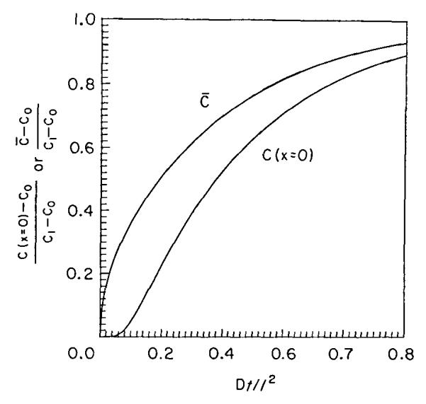
Average concentrations in the disc C̄, and concentration at the end of the disc, C(x = 0), at times normalized by multiplying time t by D/l².

Can diffusion limitation to equilibration within the discs explain their data. Yes, almost. The concentration profiles expected for diffusion into a stagnant layer are given by Crank (1956, his Figure 4.1), reproduced here as Figure 1. The numbers on the curves are the numbers of characteristic times, τ_D.

The average concentration within the disc is given by a curve, C̄, in Figure 2 (taken from Carslaw and Jaeger, 1959, their Figure 12). The curve labelled C(x = 0) gives the concentration in fluid at the far edge of the disc away from the epicardium. A curve of C̄ can be fitted through the data of Gidday’s Figure 1, and from the knowledge of the distances involved one could obtain an estimate of the effective D within the disc.

To do it the other way around is also legitimate: from the known dimensions and an estimated D, predict the result. The volume of a single disc is given as 4.8 μl and the surface area 0.636 cm², so the disc thickness, if it were pure water without matrix, would be 4.8 μl/0.636 cm² or 75.5 μm. If 1/3 of the disc is matrix then the thickness might be about 113 μm. With a diffusion coefficient for adenosine of 1.2 times that of sucrose (which I have calculated from the molecular volumes and shapes as suggested by Edward (1970), using space-filling models to determine the shapes), and a sucrose diffusion coefficient of 0.72 × 10⁻⁵ cm²/s, I estimate the adenosine diffusion coefficient to be 0.86 × 10⁻⁵ cm²/s. Then τ_D = l²/D = (113 μm)²/(0.86 × 10⁻⁵ cm²/s) = 14.8 s. The concentration-time curve using this D/l2 would fit the data of Gidday’s Figure 1 not badly, but might rise a little too fast. Maybe I underestimate the matrix volume fraction or should use a lower D if the pores are very small.

Can diffusional retardation of solute equilibration explain quantitatively their data showing low disc adenosine levels in thick discs relative to thin discs? To try this I have taken the volumes and surface area that they provide and calculated the disc or chamber thicknesses. For the discs I use my estimate of one third as the matrix fraction of the total volume (disc + water). On this basis the thicknesses for 1 and 2 discs are 113 and 226 μm; for the one mesh modified and two mesh modified discs, I calculate 256 and 377 μm, but I worry that the glue used in between the layers may reduce the cross-sectional area available for diffusion. For the chamber there is no matrix, and the thickness is 100 μl/l cm² or 1000 μm. I certainly do not expect a 1 mm layer to be well stirred: the classic study by Ginzburg and Katchalsky (1963) showed that mixing in surface layers is exceedingly slow even with high rates of stirring. In Figure 3 I have plotted the expected average concentrations in the various discs against the thicknesses for an equilibration time of 2 mins, the time the authors used. The line is labeled “Constant Source, No Barrier.” These expected average disc concentrations can be estimated from the graph in Figure 2 from the values of Dt/l², as in Table 2. The method is to calculate Dt/l² for each t and each thickness l and then slide along the line for C̄ in Figure 2 to obtain C(2 min)/C_oo. The curve I constructed on this basis (Fig. 3, filled squares) is above their observations on thicker discs, suggesting that simple diffusional resistance in the disc fluid alone is not the whole story.

FIGURE 3.

Adenosine concentrations in epicardial discs or chambers of varied thickness for 2 mins of equilibration. Open squares: data of Gidday et al., 1991; the point at 1000 μm is for a well chamber at 4 mins. Solid squares: unhindered diffusion from a constant source. Solid and open diamonds: unhindered diffusion from constant sources 100 and 200 μm deep in the epicardial surface of the heart.

TABLE 2.

Average concentrations in discs of varied thicknesses at t = 2 min

Volume of disc or chamber μl	Surface area of disc cm2	Estimated thickness of disc or chamber μm	Gidday et al. observations	Constant source
				No subepicardial layer		Subepicardial layer of thickness
						100 μm	200 μm
			$\frac{C_{2\min }}{C_{\infty }^{\ast }}$	*Dt/l2	$\frac{C_{2\min }}{C_{\infty }^{\ast }}$	$\frac{C_{2\min }}{C_{\infty }^{\ast }}$	$\frac{C_{2\min }}{C_{\infty }^{\ast }}$
0	-	0	1.00	-	1.00	1.00	1.00
4.8	0.64	113†	1.00	8.10	1.00	1.00	0.94
9.5	0.64	226†	1.12	2.02	0.99	0.93	0.80
17.0	0.64	400†	0.47	0.64	0.83	0.71	0.61
25.0	0.64	589†	0.35	0.50	0.62	0.52	0.46
100.0	1.00	1000	0.08	0.10	0.36	0.34	0.30

*Dt/l² shown only for the case with the source at the epicardial surface. $C_{\infty }^{\ast }$ represents the concentration in the thinnest epicardial disc at two minutes; C∞ for the calculations represents the equilibrium value.

† assumes disc matrix fractional volume of one third.

Submesothelial diffusion layer?

My next hypothesis was that the layer of submesothelial tissue, which is mainly loose areolar tissue between the surface of the myocardium itself and the mesothelial (endothelial) layer of visceral pericardium, might act as an additional diffusional layer between the myocardial source of adenosine and the disc. Consequently 2 lines are shown for layers with the same diffusion coefficient as in water with thicknesses of 100 and 200 μm (Fig. 3, filled and open diamonds). Neither of these curves have quite the right shape either, for the additional layer has more effect on delivery into the thin discs than on delivery into the thick discs. The curves would be lowered more toward the data if I used for this layer diffusion coefficients of the level obtained by Suenson et al. (1974) which were one quarter of the aqueous diffusion coefficient. To handle this properly we should work out the equations for a pair of diffusion layers with differing D’s, lower in the tissue than in the disc fluid. We should probably also put a hindering barrier representing the mesothelium separating them. In any case, these hypotheses that the diminished fractional equilibration can be explained by diffusion alone are in the right direction but do not offer a complete explanation. One conclusion is clear, however: the simplest of these calculations shows that the thick discs cannot be equilibrated in the time allowed, but the thinnest disc can be.

Mesothelial resistance

Gidday et al. consider that the mesothelium is not a significant barrier. Hanley et al. (1983) rubbed on it to destroy its contiguity yet found no difference in equilibration time. If we assume that there is no transport into mesothelial cells themselves, then we can ask if the transmembrane conductance can be high enough to account for this, or must there be transcellular transport as well as transport through the clefts. The conductance is given by permeability-surface area product; if it is the same as for sucrose penetrating interendothelial clefts, about l ml g⁻¹ min⁻¹, then the permeability, P, is about 3 × 10⁻⁴ cm/s. This is of the same order as is D/l for the thin disc, which is 0.86 × l0⁻⁵/113 × l0⁻⁴ or 7.6 × 10⁻⁴ cm/s, and is enough to explain the difference between my too small estimate of the equilibration time or τ_D compared to their observations. I would conclude that the mesothelial resistance is small and evident only when observations are made at short times.

Submesothelial depletion

Gidday et al. have proposed that the diffusion into the discs of larger volume leads to depletion of the adenosine concentration in the submesothelial layer. This is very likely; after all the volume of the well chamber is 100μl, while that of the submesothelial 100 μm thick layer is only 10μd, and under the discs only 6.4μ1. In the first minute a large fraction of the solute in the layer would be lost into the disc fluid, a serious depletion. This depletion would certainly persist for some minutes for the larger volume discs. Replenishment of the local [Ado]_isf must come from the local cells, not from the vascular space which rapidly supplies the sucrose. The depletion is greater when the diffusion coefficients within the tissue are smaller than those in the disc fluid, exacerbating the problem by adding the diffusional resistance in disc to that in the tissue and prolonging the time to equilibration. Depletion of a local region is, however, strictly a transient phenomenon. Steady state will be reached only when the ISF has been replenished and the disc concentration equals the ISF concentration.

Steady state and mass balance

Gidday et al. believed that they had reached a steady state in which the [Ado]_isf was lower than at t = 0 and the disc had equilibrated with this lower concentration. This idea ignores the fact that there will be continuing fluxes until there is no gradient, and the fact that a gradient cannot persist unless there is consumption. They assume that consumption within the disc is zero; if this assumption is correct, their idea of a steady state violates a fundamental conservation principle.

How do we go about avoiding such pitfalls. There are two parts to the answer. The first is figuring out how the mistake is made, the second is figuring out how to make checking easier. How the error occurred is probably now clear: by using the exponential or mixing chamber idea, and not making a series of observations on thick discs like they did on thin discs, they thought the time was adequate for equilibration.

If we accept the premise that no adenosine is chemically degraded in the disc fluids or interstitium, then we can state unequivocally that steady state will be achieved with a concentration in the disc fluid that exactly matches that in the subendothelial layer. Diffusional retardation of molecular movement governs the rate of achievement of this state but has no influence on the outcome. The only way there can be a standing gradient n concentrations between the myocardium and the disc if there is consumption of adenosine in the disc fluid itself. Binding to disc elements cannot do this either, for while diffusion is slowed by the presence of binding sites (Safford and Bassingthwaighte, 1977), this can only act to slow the rate of equilibration, not to change its level.

To avoid such traps I have some simple “gimmicks” which work for me. One is to make sure that the units of everything in a calculation balance out exactly; this means accounting for conversions using 60 s/min and such transformations that are easily forgotten. A second gimmick is to follow the rule of mass balance across an interface or into and out of a chamber or organ:

$$\text{Rate of change of amount contained}=\text{Flux in}-\text{Flux out},$$ (5)

and sticking carefully to moles, or equivalent. For the case in point, the amount in the disc is C_disc times V_disc, and the fluxes can be written down from the concentrations and the conductances. For the stirred mixing chamber idea, these would be simply:

$$V_{\mathrm{disc}}•\mathrm{d}{C}_{\mathrm{disc}}∕\mathrm{d}t=\mathrm{G}•C_{\mathrm{isf}}-\mathrm{G}•C_{\mathrm{disc}}-\text{Consumption}$$ (6)

where the units are V_disc, ml; C, mols/ml; G is the conductance, ml/s, and Consumption has the units moles/s, the same units as for the left side of the equation. (To explain G in diffusional terms consider it as representing a fluid layer or a membrane where G = DS/l or PS, where S is surface area and P permeability.) One reaches a steady state only when C_disc is not changing, so dC_disc/dt and the left side of the equation equal zero. If consumption inside the disc is zero, then the only circumstance allowing the right side of the equation to become zero is when C_isf = C_disc. This steady state is therefore also an equilibrium state.

If consumption were not zero, then in the steady state the consumption must exactly match the excess flux into the disc:

$$\text{Consumption}=\mathrm{G}•C_{\mathrm{isf}}-\mathrm{G}•C_{\mathrm{disc}},$$ (7)

GC_isf is the unidirectional flux from ISF to disc; GC_disc is the back flux. The presence of any adenosine deaminase in the disc would pull down the steady state concentration. Therefore, if there is any chance of adenosine degradation via enzymes such as a deaminase in the ISF, I would prefer putting EHNA, a deaminase blocker, into the fluid, to relying on the observation that a chemical test failed to detect deaminase.

Adenosine concentrations in the interstitial fluid

All this reanalysis fails to resolve the questions extant about how to measure C_isf either locally or globally. The disc and well techniques can at best give estimates of local concentrations at surfaces. In general the disc and well techniques give values higher than one would calculate from the venous outflow adenosine concentrations. Table 1 shows the wide diversity of results: transudate samples were nearly 200 nm, epicardial disc measures averaged 154,280 and 470 nm, while estimates from capillary transport techniques based on indicator dilution studies, which should give values averaged over the whole heart, were 3 to 12 nm. This disparity led Gorman et al. (1991) to question their physiological model for capillary-tissue exchange, and to test whether or not there was a specialized uptake mechanism for adenosine within the clefts between endothelial cells. Their answer was that intracleft uptake would only reconcile their analyses with the transudate and epicardial disc estimates if the density of uptake sites within the capillary endothelial clefts was several times higher than the density of sites on the capillary luminal surface of the endothelial cell. Because determining the rate of uptake within clefts less than 20 nm wide separately from the neighboring free surfaces, luminal and abluminal, is not technically possible, we remain dependent upon direct sampling techniques for trying to sort out the possibilities. It is therefore important that methods like the transudate and thin epicardial discs be used, even if they give only local surface information.

If there is not a specialized uptake mechanism for adenosine in capillary interendothelial clefts, an open question, then it might be concluded that the high epicardial transudate levels are either some rather odd artifact, or there is something special about the epicardial surface or about the way it responds to exposure. Could high adenosine concentrations locally be related to the neural plexuses beneath the pericardial surface? Plexuses are found in the subendocardial region as well. Certainly sympathetic stimulation raises adenosine levels, and while I have assumed that this comes from myocytes, the neurons have high ATP levels (as do endothelial cells) and have the capacity to produce all the adenosine that is to be found. At the highest levels, about 1000 nm adenosine, the cardiac content of interstitial adenosine is miniscule compared to intracellular ATP levels.

The possibility that discs and transudates represent local and perhaps artifactually high epicardial levels must be balanced against the alternative that the capillary transport analysis is wrong, underestimating ISF concentrations. The closest to direct comparisons are the nice analyses of Mohrman and Heller (1990), and they initiated the study of adenosine uptake in the cleft, the Appendix in Gorman et al. (1991). The capillary transport data are fairly strong, the data being now quite extensive and reproducible. The measures of capillary cleft and endothelial permeability are solid, while those on permeability of the myocyte and of the abluminal surface of the endothelial cell are relatively weak. The cleft itself is a mystery, but since the surface area is about one twelfth of the total, the influence is not likely very great. Table 1 lists only guinea pig data on isolated hearts perfused without erythrocytes, preparations which are good for testing specific mechanisms but which are not in a normal physiological state. A difference exists between studies: the capillary transport studies all had low venous adenosine concentrations whereas those using discs or transudates, with one exception, showed relatively high venous levels. It is therefore possible that differences in conditions in the various studies may be the sole basis of differences in estimated ISF concentrations, with all techniques except the thick discs and well chambers being correct.

Temporal and spatial heterogeneity of adenosine concentrations

Gidday et al. report large temporal fluctuations and large differences between two nearby samples obtained simultaneously. These are their most important observations. The variation is greater than measurement error. The temporal component of the variation is estimated to have a coefficient of variation of nearly 50 %, more variation than we find in spatial distributions in flows, but certainly compatible with the variation that is predicted by fractal extrapolation (Bassingthwaighte, King and Roger, 1989) down to regions of the sizes being sampled by the disc method, of the order of 5 to 20 μl. Do the temporal fluctuations in adenosine correlate with fluctuations in flows? What one would really like to know next is the relationship between the local flows and the local adenosine levels, with knowledge of the temporal fluctuations thrown in for good measure. This might be possible with the thin discs and with microspheres for flows, but the data collection and analysis problem with the disc technique is sufficiently formidable that it will be difficult to obtain large sets of data. We need data on local flows (e.g., with microspheres) along with [Ado]_isf in the same pieces.

The SAH method of Deussen, Borst and Schrader (1988) may give the best opportunity. The technique is to drive the S-adenosylhomocysteine hydrolase reaction backward from its normal net flux by raising the blood levels of tracer homocysteine. Having excess homocysteine inside the myocytes then serves as a bioassay for free intracellular adenosine, trapping it inside the cell as SAH, which is too hydrophilic to escape from the cell. Tissue sampling can then be done for measurement of tracer SAH content along with microsphere measurement of the local flow. The technique is an integral one, requiring the accumulation of SAH over at least several minutes. The method is probably sensitive enough to be useful in normal states when adenosine loss from ATP is minimal, and is clearly valuable when adenosine levels rise in hypoxia and ischemia. Even so, this is an assay for intracellular, not interstitial adenosine, and again one would have to resort to model analysis to interpolate between cytosolic and venous adenosine levels.

Conclusion

1. Methods for measuring interstitial adenosine concentrations are indirect.

2. Thin epicardial porous discs equilibrate rapidly and can be relied on to measure local subepicardial [Ado]_isf.

3. Thicker discs and epicardial chambers take long times to equilibrate and are more subject to error due to adenosine degradation. These should not be used.

4. Local epicardial [Ado]_isf levels appear to be much higher than global levels estimated from the venous concentrations and capillary transport parameters.

5. All methods show [Ado]_isf to be much higher than in the venous outflow.

6. Spatial and temporal heterogeneity in [Ado]_isf is probably real, not due to methodological error. The relationship between the heterogeneous [Ado]_isf and the heterogeneous regional myocardial blood flows is unknown but is important to our understanding of myocardial metabolism/flow relationships and myocardial vasoregulation.

References

- Bassingthwaighte JB, Wang CY, Gorman M, De Witt D, Chan IS, Sparks HV. Endothelial regulation of agonist and metabolite concentrations in the interstitium. In: Yudilevich DL, Mann GE, editors. Carrier-Mediated Transport of Solutes from Blood to Tissue. Longman; New York: 1985. pp. 191–203. [Google Scholar]
- Bassingthwaighte JB, King RB, Roger SA. Fractal nature of regional myocardial blood flow heterogeneity. Circ Res. 1989;65:578–590. doi: 10.1161/01.res.65.3.578. [DOI] [PMC free article] [PubMed] [Google Scholar]
- Berne RM. Cardiac nucleotides in hypoxia: possible role in regulation of coronary blood flow. Am J Physiol. 1963;204:317–322. doi: 10.1152/ajplegacy.1963.204.2.317. [DOI] [PubMed] [Google Scholar]
- Carslaw HS, Jaeger JC. Conduction of Heat in Solids. Clarendon Press; Oxford: 1959. [Google Scholar]
- Crank J. The Mathematics of Diffusion. Clarendon Press; Oxford: 1956. [Google Scholar]
- Decking UK, Juengling ME, Kammermeier H. Am J Physiol. Heart Circ Physiol. 1988;254(23):H1125–H1132. doi: 10.1152/ajpheart.1988.254.6.H1125. Interstitial transudate concentration of adenosine and inosine in rat and guinea pig hearts. [DOI] [PubMed] [Google Scholar]
- Deussen A, Borst M, Schrader J. Formation of S-adenosylhomocysteine in the heart. I. An index of free intracellular adenosine. Circ Res. 1988;63:240–249. doi: 10.1161/01.res.63.1.240. [DOI] [PubMed] [Google Scholar]
- Edward JT. Molecular volumes and the Stokes-Einstein equation. J Chem Ed. 1970;47:261–270. [Google Scholar]
- Gidday JM, Kaiser DM, Rubio R, Berne RM. Heterogeneity and sampling volume dependence of epicardial adenosine concentrations. J Mol Cell Cardiol. 1992;24:351–364. doi: 10.1016/0022-2828(92)93190-u. [DOI] [PubMed] [Google Scholar]
- Ginzburg BZ, Katchalsky A. The factional coefficients of the flows of non-electrolytes through artificial membranes. J Gen Physiol. 1963;47:403–418. doi: 10.1085/jgp.47.2.403. [DOI] [PMC free article] [PubMed] [Google Scholar]
- Gorman MW, Wangler RD, Bassingthwaighte JB, Mohrman DE, Wang CY, Sparks HV. Interstitial adenosine concentration during norepinephrine infusion in the isolated guinea pig hearts. Am J Physiol. 1991:H901–909. doi: 10.1152/ajpheart.1991.261.3.H901. Heart Circ Physiol 30. [DOI] [PMC free article] [PubMed] [Google Scholar]
- Hanley F, Messina LM, Baer RW, Uhlig PN, Hoffman JIE. Am J Physiol. (Heart Circ Physiol. 1983;245(14):H327–H335. doi: 10.1152/ajpheart.1983.245.2.H327. Direct measurement of left ventricular interstitial adenosine. [DOI] [PubMed] [Google Scholar]
- Headrick JP, Matherne GP, Berr SS, Han DC, Berne RM. Am J Physiol. Heart Circ Physiol. 1991;260(29):H165–H172. doi: 10.1152/ajpheart.1991.260.1.H165. Metabolic correlates of adenosine formation in stimulated guinea pig heart. [DOI] [PubMed] [Google Scholar]
- Heller LJ, Mohrman DE. Estimates of interstitial adenosine from surface exudates of isolated rat hearts. J Mol Cell Cardiol. 1988;20:509–523. doi: 10.1016/s0022-2828(88)80078-6. [DOI] [PubMed] [Google Scholar]
- Mohrman DE, Heller LJ. Am J Physiol. Heart Circ Physiol. 1990;259(28):H772–H783. doi: 10.1152/ajpheart.1990.259.3.H772. Transcapillary adenosine transport in isolated guinea pig and rat hearts. [DOI] [PubMed] [Google Scholar]
- Safford RE, Bassingthwaighte JB. Calcium diffusion in transient and steady states in muscle. Biophys J. 1977;20:113–136. doi: 10.1016/S0006-3495(77)85539-2. [DOI] [PMC free article] [PubMed] [Google Scholar]
- Suenson M, Richmond DR, Bassingthwaighte JB. Diffusion of sucrose, sodium, and water in ventricular myocardium. Am J Physiol. 1974;227:1116–1123. doi: 10.1152/ajplegacy.1974.227.5.1116. [DOI] [PMC free article] [PubMed] [Google Scholar]
- Tietjan CS, Tribble CG, Gidday JM, Phillips CL, Belardinelli L, Rubio R, Berne RM. Am J Physiol. Heart Circ Physiol. 1990;259(28):H1471–H1476. doi: 10.1152/ajpheart.1990.259.5.H1471. Interstitial adenosine in guinea pig hearts: an index obtained by epicardial disks. [DOI] [PubMed] [Google Scholar]
- Wangler RD, Gorman MW, Wang CY, De Witt DF, Chan IS, Bassingthwaighte JB, Sparks HV. Am J Physiol. Heart Circ Physiol. 1989;257(26):H89–H106. doi: 10.1152/ajpheart.1989.257.1.H89. Transcapillary adenosine transport and interstitial adenosine concentration in guinea pig hearts. [DOI] [PMC free article] [PubMed] [Google Scholar]
- Yipintsoi T, Dobbs WA, Jr, Scanlon PD, Knopp TJ, Bassingthwaighte JB. Regional distribution of diffusible tracers and carbonized microspheres in the left ventricle of isolated dog hearts. Circ Res. 1973;33:573–587. doi: 10.1161/01.res.33.5.573. [DOI] [PMC free article] [PubMed] [Google Scholar]