Looping Probabilities in Model Interphase Chromosomes

Abstract

Fluorescence in-situ hybridization (FISH) and chromosome conformation capture (3C) are two powerful techniques for investigating the three-dimensional organization of the genome in interphase nuclei. The use of these techniques provides complementary information on average spatial distances (FISH) and contact probabilities (3C) for specific genomic sites. To infer the structure of the chromatin fiber or to distinguish functional interactions from random colocalization, it is useful to compare experimental data to predictions from statistical fiber models. The current estimates of the fiber stiffness derived from FISH and 3C differ by a factor of 5. They are based on the wormlike chain model and a heuristic modification of the Shimada-Yamakawa theory of looping for unkinkable, unconstrained, zero-diameter filaments. Here, we provide an extended theoretical and computational framework to explain the currently available experimental data for various species on the basis of a unique, minimal model of decondensing chromosomes: a kinkable, topologically constraint, semiflexible polymer with the (FISH) Kuhn length of l_K = 300 nm, 10 kinks per Mbp, and a contact distance of 45 nm. In particular: 1), we reconsider looping of finite-diameter filaments on the basis of an analytical approximation (novel, to our knowledge) of the wormlike chain radial density and show that unphysically large contact radii would be required to explain the 3C data based on the FISH estimate of the fiber stiffness; 2), we demonstrate that the observed interaction frequencies at short genomic lengths can be explained by the presence of a low concentration of curvature defects (kinks); and 3), we show that the most recent experimental 3C data for human chromosomes are in quantitative agreement with interaction frequencies extracted from our simulations of topologically confined model chromosomes.

Introduction

Genes that are spatially close can be regulated together (1–4), even if they are located in different parts of a chromosome (α-globin locus (5)) or on different chromosomes (olfactory receptor genes (6)). Attempts to rationalize the mechanisms by which loci come together and form transient associations (3) require an understanding of the local and the large-scale spatial organization and dynamics of chromosomes in interphase nuclei.

Experimentally, the large length-scale organization of interphase chromosomes can be investigated by marking of specific DNA sequences via fluorescence in situ hybridization (FISH) (2,7,8) (Fig. 1). Given the low spatial resolution of FISH, contacts between chromatin fibers are more readily identified using high-resolution techniques such as cryo-FISH (9) and chromosome conformation capture (3C) (10,11). 3C and other 3C-based technologies, as for instance 5C (12) and the very recent Hi-C (13), use formaldehyde cross-linking and locus specific polymerase chain reaction to detect physical contacts between genomic loci (Fig. 2). In principle, 3C can provide quantitative information about interaction frequencies between arbitrary chromatin sites.

Figure 1.

Mean-square internal distances R²(|N₂ − N₁|) between targeted interphase chromosome sites at N₁ and N₂ mega-basepairs (Mbp) from one chosen end of the fiber: comparison between currently available FISH data and our model for interphase chromosomes (for details, see (19)). (Brown squares) FISH data for yeast chromosomes (8). (Violet squares) FISH data for human chromosomes (7). The short length-scale distances (up to ≈4 Mbp) were measured on the (nearly equilibrated) end region 4p16.3 on human chromosome 4 (19). (Black lines) Exact wormlike chain (WLC) expression, Eq. 1: l_K = 300 nm (solid line) and l_K = 56 nm (dashed line). (Red line) Model human chromosomes. (Cyan line) Model human chromosomes with N₁ = 0. (Green line) Model yeast chromosomes.

Figure 2.

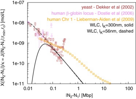
Rescaled interaction frequencies X(|N₂ − N₁|)/κ between chromosome sites at N₁ and N₂ mega-basepairs (Mbp) from one chosen end of the fiber can be quantitatively detected by chromosome conformation capture (3C). (Brown squares) 3C interaction frequencies between sites exploring the entire contour length (L_c ≈ 0.3 Mbp) of chromosome 3 in yeast Saccharomyces cerevisiae (10). (Violet squares) 5C interaction frequencies between sites exploring the (silenced) human β-globin locus (12). (Orange squares) Hi-C interaction frequencies between sites on human chromosome 1 (13). (Black lines) Interpolation formula for a WLC proposed by Shimada and Yamakawa (22), Eq. 5: l_K = 300 nm (solid line) and l_K = 56 nm (dashed line). Due to the unknown efficiency of the cross-linking reaction, 3C does not measure the absolute value of the interaction frequencies and we have shifted the experimental data according to a convention discussed in 3C Interaction Frequencies X(L) and Chain Looping Probabilities J(L; r_min, r_c).

To infer the (local) structure of the chromatin fiber or to distinguish functional interactions from random colocalization, it is useful to compare FISH and 3C data to predictions from statistical fiber models. For example, the 3C contact frequencies between sites at opposite ends of the yeast chromosome largely exceed theoretical predictions (Fig. 2) and their interpretation in terms of a biologically functional ring formation (10) corresponds well to the independent observation of telomere pairing for yeast chromosome 3 as a consequence of the specific anchoring of chromosome ends to the nuclear envelope (14). Other observed deviations from the equilibrium statistics of wormlike chains such as the segregation of chromosomes into territories have been alternatively ascribed to biologically controlled contacts between chromatin fibers (random-walk/giant-loop model (7), multiloop/subcompartment model (15), random loop model (16), thermodynamic models (17)) or to generic polymer effects (i.e., the “crumpled globule” (18)). We have recently used computational techniques to provide quantitative evidence supporting the crumpled-globule model (19). We have carefully mapped the relevant length- and timescales in eukaryotic nuclei onto a minimal polymer model of decondensing chromosomes obeying topological (entanglement) constraints. Our simulations demonstrated the emergence of the fractal structures predicted by the crumpled globule model. In particular, we quantitatively reproduced FISH observations for the existence of territories and their shapes, for the observed fiber dynamics, and for spatial distances between marked chromosome sites for human, Drosophila, and budding yeast chromosomes (Fig. 1). The observation that the general folding of chromatin fibers inside interphase nuclei may follow from generic polymer behavior obviously does not exclude the presence of specific, biologically evolved contacts. The point is that, similarly to the example for yeast cited above, functional contacts within and between chromosome territories may be identified via a comparison to the predictions of a suitable generic model.

Available expressions (20,21) for looping probabilities are largely based on generalizations of the classical result by Shimada and Yamakawa (22) for isolated, wormlike semiflexible polymers with infinitesimal capture radius in thermal equilibrium (Fig. 2, Eq. 5).

In this article, we improve on the theoretical description of nonspecific chromosomal contacts. We quantify the effects of finite chromatin fiber thickness, facilitated kinking, and territory formation on the expected contact statistics. In particular, we extend the theoretical description of interphase chromosomes in several directions:

Due to the smaller aspect ratio of chromatin, the assumption of an infinitesimal capture radius is more problematic than in the case of DNA. Here we present a reliable expression for looping probabilities in equilibrated wormlike chains with finite diameters or capture radii, which strongly modifies the expected behavior for small genomic distances. The expression is derived from our recent results for the end-to-end distance probability density for semiflexible polymer chains (23), which incorporate all analytically known limiting cases.

Closer inspection of the theoretical curves in Figs. 1 and 2 reveals an apparent inconsistency: locally (i.e., up to genetic distances of 1 Mbp), the FISH data for mean-square spatial distances are in excellent agreement with the wormlike chain model for a Kuhn length l_K ≈ 300 nm (8) (Fig. 1). In contrast, the 3C data seem to suggest a much softer fiber (10) (l_K ≈ 56 nm, Fig. 2). Building on recent results for DNA (24,25), we show that this apparent conflict can be resolved by assuming a small concentration of kinks along the chromatin fiber.

Whereas small chromosomes (as in yeasts) effectively equilibrate, large chromosomes (as in humans) do not mix and remain confined to discrete territories. In Rosa and Everaers (19), we compared the predictions of our minimal model of decondensing chromosomes to available FISH data. Here we extend the comparison to recent experimental 3C data for human chromosomes (13).

The objective of treating these independent aspects of chromosome statistics in a single publication is to establish a unique minimal polymer model of decondensing DNA, which can be compared to FISH and 3C data for all species. The article is organized as follows: Theory of Wormlike Chain Looping reviews the theory of wormlike chains. Model and Methods describes our simulation model of (topologically confined) wormlike and kinkable chromatin fibers and defines the methods employed. We then present our results and conclude by a short discussion.

Theory of Wormlike Chain Looping

As in our previous work (19), we model the (30-nm) chromatin fiber as a semiflexible polymer chain. Fiber statistics at equilibrium is described by the so-called wormlike chain (WLC) model, which is characterized by a crossover from rigid rod to random coil behavior at a characteristic length-scale, i.e., the Kuhn length l_K = 50–300 nm of the 30-nm chromatin fiber (8,10). Consider two points located at N₁ and N₂ mega-basepairs (Mbp) from one chosen end of the fiber. They are separated by L = |N₁ − N₂| × 10 μm/Mbp along the contour of the chromatin fiber (26). On small scales, the fiber is essentially stiff with a mean-square spatial distance R²(L ≪ l_K) = L². On large scales, fibers are bent by thermal fluctuations with R²(L) = Ll_K. The full crossover is described by (27)

$$R^2\left(L\right)=\frac{l_{\mathrm{K}}^2}{2}\left(\frac{2L}{l_{\mathrm{K}}}+e^{-2{\mathrm{L}/\mathrm{l}}_{\mathrm{K}}}-1\right)$$ (1)

(black lines, Fig. 1). In particular, Eq. 1 holds in the bulk of semidilute solutions where chains strongly overlap.

An interpolation formula for chain looping

In this work, two sites at mutual genomic separation L along the same chromatin fiber are said to form a contact if their spatial distance r becomes smaller than a suitable reaction distance r_c. For a polymer fiber with excluded volume interactions (like the one considered here), the physical meaning of r corresponds to the distance between two points on the center-line of the fiber (see Average Square Internal Distances for Simulated Chromosomes, and Chain Looping Probabilities for Simulated Chromosomes).

The corresponding looping probability J(L;r_min,r_c) is defined by (21)

$$J\left(L;r_{\text{min}},r_{\mathrm{c}}\right)=\frac{1}{V_{\text{int}}\left(r_{\mathrm{c}}\right)}\underset{{\mathrm{r}}_{\text{min}}}{\overset{{\mathrm{r}}_{\mathrm{c}}}{\int }}{p}_{\mathrm{L}}\left(r\right)4\pi r^{2}dr.$$ (2)

Here, p_L(r) is the probability density of the internal distances between chromatin sites at mutual genomic separation L; r_min ≈ 40 nm is the distance of minimum approach (which takes into account excluded volume effects) and V_int(r_c) = 4πr_c³/3 is the reacting volume. (Excluded volume interactions prevent fibers from coming closer than r_min and, for our chromatin model, one would naively expect r_min = 30 nm. This is not the case. In fact, because of the large fiber stiffness (l_K = 300 nm), at short length-scales chromatin fibers behave like rigid rods, whose reciprocal excluded volume is ≈l_K²σ (28). Then, the corresponding excluded volume per monomer is $\approx l_{\mathrm{K}}{\sigma }^2\approx \frac{4\pi }{3}{r}_{\text{min}}^3$ or, r_min ≈ 40 nm.)

The expression J(L;r_min, r_c) gives directly the concentration of one binding site in proximity of the other. For experimental convenience, J(L;r_min, r_c) is usually expressed in moles per liter (mol/L) where 1 mol/L ≈ 0.6 nm⁻³.

It is useful to rewrite Eq. 2 as

$$J\left(L;r_{\text{min}},r_{\mathrm{c}}\right)=J\left(L;0,r_{\mathrm{c}}\right)-\frac{V_{\text{int}}\left(r_{\text{min}}\right)}{V_{\text{int}}\left(r_{\mathrm{c}}\right)}J\left(L;0,r_{\text{min}}\right),$$ (3)

which reduces the problem to computing the function J(L;0, r), i.e., the looping probability of a phantom chain at finite contact radius r.

In the Gaussian long chain limit, J(L;0, r) is given by a simple exact expression. In this case, p_L(r) is described by the three-dimensional Gaussian function p_L(r) = (3/2πLl_K)^3/2 exp(−3r²/2Ll_K) (27) and J_GC(L;0, r) is given by

$$J_{\text{GC}}\left(L;0,r\right)=\left[\text{erf}\left(\sqrt{\frac{3r^2}{2L{l}_{\mathrm{K}}}}\right)-\frac{2}{{\pi }^{1/2}}\sqrt{\frac{3r^2}{2L{l}_{\mathrm{K}}}}\exp \left(-\frac{3r^2}{2L{l}_{\mathrm{K}}}\right)\right]/\frac{4}{3}\pi r^3,$$ (4)

where

$$\text{erf}\left(x\right)=\frac{2}{{\pi }^{1/2}}\underset{0}{\overset{\mathrm{x}}{\int }}\exp \left(-y^2\right)dy.$$

Because L ≫ l_K, Eq. 4 simplifies further to

$$J_{\text{GC}}\left(L;0,r\right)\approx \frac{1}{{\mathrm{l}}_K^3}{\left(\frac{3}{2\pi {L/\mathrm{l}}_K}\right)}^{3/2}.$$

No explicit expression for p_L(r) is available, current proposed formulas being 1), only valid around full chain extension (29); 2), mean-field-like (30,31); or, 3), otherwise computationally very demanding (32).

Recently, we have proposed the following interpolation expression p_L^I(r) for the end-to-end distance probability density of a semiflexible polymer chain, which is valid for all Kuhn lengths and end-to-end distances (23) (see Appendix for a definition of the different quantities involved):

$$p_{\mathrm{L}}^{\mathrm{I}}\left(r\right)=J_{\text{SY}}\left(L\right){\left(\frac{1-c{\rho }^2}{1-{\rho }^2}\right)}^{5/2}\exp \left(\frac{\sum _{\mathrm{i}=-1}^0\sum _{\mathrm{j}=1}^3{c}_{\text{ij}}{\lambda }^{\mathrm{i}}{\rho }^{2\mathrm{j}}}{1-{\rho }^2}\right)\times \exp \left(-d\lambda \frac{ab\left(1+b\right){\rho }^2}{1-b^2{\rho }^2}\right)\times I_0\left(-d\lambda \frac{a\left(1+b\right)\rho }{1-b^2{\rho }^2}\right)\text{.}$$ (5)

Equation 5 provides to a good approximation the end-to-end distance probability density of a wormlike chain over the entire range of lengths and end-to-end distances (23). In this article, we use Eq. 5 together with Eqs. 2 and 3, to obtain a simple and accurate extension of the Shimada and Yamakawa ring-closure probability to finite contact radii.

We conclude this section by remarking that the theory above is valid only for equilibrated, homogeneously bending, locally straight chromatin fibers. Real fibers exhibit local defects (33). Moreover, in species with chromosomes which are ≳5 Mbp, topological constraints or entanglements prevent equilibration during the typical cell cycles leading to chromosome segregation (19). The territory structure resembles a crumpled-globule, with a fractal structure: the average square internal distance R²(L) between fiber loci at mutual genomic separation L is given by R²(L) ∼ L^2/3, which contrasts the R²(L) ∼ L equilibrium behavior (18). In the following, we employ molecular dynamics (MD) computer simulations to investigate the effects of entanglements, incomplete equilibration, and fiber kinking on intrachromosomal contacts.

Model and Methods

Fiber models

To model the 30-nm chromatin fiber, we have used the generic bead-spring polymer model of Kremer and Grest (34): the model takes into account the connectivity, stiffness, excluded volume, and local topology conservation of the fiber. As in our previous work (19), we have worked at the typical nuclear density of ≈0.012 bp/nm³ = 12 Mbp/μm³, or ≈6 × 10⁻⁶ mol/L.

Chains are composed of N_b interacting beads of diameter σ = 30 nm. Each bead is thus equivalent to 3000 basepairs (26).

There are three types of interactions: U_LJ, U_FENE, and U_stiff. U_LJ is a shifted, purely repulsive Lennard-Jones potential

$$U_{\text{LJ}}=\{\begin{array}{l}4\varepsilon \left[{\left(\sigma /r_{\text{ij}}\right)}^{12}-{\left(\sigma /r_{\text{ij}}\right)}^6+1/4\right],r_{\text{ij}}\le \sigma 2^{1/6}\hfill \\ 0,r_{\text{ij}}>\sigma 2^{1/6}\hfill \end{array}$$ (6)

between any two monomers. The potential

$$U_{\text{FENE}}=\{\begin{array}{l}-0.5k{R}_0^2\ln \left[1-{\left(r_{\text{ij}}/R_0\right)}^2\right],r_{\text{ij}}\le R_0\hfill \\ 0,r_{\text{ij}}>R_0\hfill \end{array}$$ (7)

gives the additional interaction between nearest neighbors along the chain. Simulation parameters are given by R₀ = 1.5σ, k = 30.0ɛ/σ² and temperature k_BT = 1.0ɛ (34).

Fiber stiffness is modeled by U_stiff(θ), where θ is the angle formed by the oriented unit vectors of two consecutive bonds. In this work, we discuss the following three expressions for U_stiff(θ) (Fig. 3):

$$U_{\text{stiff}}^{\left(\text{a}\right)}\left(\theta \right)=\frac{k_{\theta }}{2}{\theta }^2,$$ (8)

$$U_{\text{stiff}}^{\left(\mathrm{b}\right)}\left(\theta \right)=k_{\theta }\left(1-\cos \theta \right),$$ (9)

$$U_{\text{stiff}}^{\left(\mathrm{c}\right)}\left(\theta \right)=\frac{k_{\theta }}{2}{\theta }^2{\left(\tanh \left[{\left(\frac{2E_{\mathrm{s}}}{k_{\theta }{\theta }^2}\right)}^{10}\right]\right)}^{1/10}.$$ (10)

Figure 3.

Potentials used to model the stiffness of the fiber with a Kuhn length l_K ≈ 300 nm (k_θ = 5 k_BT): U_stiff (θ) = k_θ/2 θ² (Eq. 8, red line); U_stiff (θ) = k_θ (1 − cos θ) (Eq. 9, green line); $U_{\text{stiff}}\left(\theta \right)=k_{\theta }/2{\theta }^2{\left(\tanh \left[{\left(2{\mathrm{E}}_{\mathrm{s}}/{\mathrm{k}}_{\theta }{\theta }^2\right)}^{10}\right]\right)}^{1/10}$, and E_s = 5.2 k_BT (Eq. 10, blue line).

Equations 8 and 9 are standard choices in modeling semiflexible fibers. In particular, Eq. 9 was used in our previous work (19).

We have chosen the analytical functional form given by Eq. 10 as a practical-to-implement expression to simulate semiflexible polymers with localized sharp bendings (kinks). Equation 10 keeps the general features of the kinkable WLC potential discussed in Wiggins et al. (24): it has the same small-θ behavior of Eqs. 8 and 9 (≈k_θ/2 θ²) and saturates (= E_s) at angles θ ≳ π/2 (Fig. 3, blue line). Clearly, other choices for the effective bending potential are possible and there are no limits to the complexity of effects that contribute to it (e.g., on large scales, local cooperative unstacking of nucleosomes (35) could look like kinking similar to the related discussion for DNA where the nonlinear fiber stiffness (24,36) and local melting (25) are expected to lead to the same effective large-scale behavior). In general, for the large-scale properties, only the second moment of the bend angle distribution matters. For the rare events that require sharp bending, only the maximum energy penalty for bending matters. The effective bending potential Eq. 10 is a convenient expression that captures both of these essential limits.

Pragmatically defining a kink as two consecutive bonds making an angle θ ≥ π/2, the kinking probability per unit length ζ is given by

$$\begin{array}{c}\zeta =\frac{1}{\sigma }\frac{\underset{\pi /2}{\overset{\pi }{\int }}d\theta \sin \theta e^{-\beta U_{\text{stiff}}^{\left(\mathrm{c}\right)}\left(\theta \right)}}{\underset{0}{\overset{\pi }{\int }}d\theta \sin \theta e^{-\beta U_{\text{stiff}}^{\left(\mathrm{c}\right)}\left(\theta \right)}}\\ \approx \frac{\beta k_{\theta }}{\sigma }{e}^{-\beta E_{\mathrm{s}}}\approx \frac{l_{\mathrm{K}}}{2{\sigma }^2}{e}^{-\beta E_{\mathrm{s}}}\end{array}\text{.}$$ (11)

In similarity to the Kuhn length l_K, the kinking probability ζ is a physical observable, while k_θ and E_s are parameters that depend on the discretization of the fiber model. E_s can be related to the free energy penalty of ≈9 k_BT for kinking a short (0.01 Mbp) chromatin filament between two particular nucleosome core particles (37). As each nucleosome core particle contains ≈200 bp (38), Eq. 11 gives a kink density of ≈46 kinks/Mbp. Accurate fitting of the experimental 3C data to our simulations gives the smaller value of ≈10 kinks/Mbp, which has been used throughout the text.

Simulation details

We performed MD simulations, using an integration time t_int = 0.012τ_MD, where τ_MD = σ(m/ɛ)^1/2 is the Lennard-Jones time and m is the bead mass (34). As we showed in our previous work, mapping the single-monomer dynamics to the mean-square displacement of an active gene in yeasts fixes τ_MD = 0.02 s (19).

Initial configurations, decondensation, and equilibration

Model yeast chromosomes. We performed constant volume simulations of a model system of six polymer chains of individual contour length L_c = 1.05 Mbp. Because yeast chromosomes can actually equilibrate (19), we have chosen a system of equilibrated chains as the initial condition. Model human chromosomes. We performed constant pressure simulations of a model system of four polymer chain of individual contour length L_c = 97.2 Mbp. Chains were initially prepared in a mitotic-like state, as described in our previous work (19), and fiber decondensation was simulated up to time t = 2.4 × 10⁵ s (≈3 days) using bending potential U_stiff(θ) = k_θ(1 − cos θ) (Eq. 9). The configuration stored at the end of this simulation was used as the initial state for both the simulations with bending potentials Eqs. 8 and 10.

Finally, robustness of results for model human chromosomes has been checked against simulations of decondensing ring polymers of different linear sizes: L_c = 2 × 2.7, × 48.6, and × 97.2 Mbp (19).

A summary of the investigated model systems, the employed bending potential, and the length of the individual simulation runs is given in Table 1.

Table 1.

Simulation times for model yeast and human chromosomes

Ustiff(θ)	$\frac{{\mathrm{k}}_{\theta }}{2}{\theta }^2$	kθ(1 − cos θ)	$\frac{{\mathrm{k}}_{\theta }}{2}{\theta }^2{\left(\tanh \left[{\left(\frac{2{\mathrm{E}}_{\mathrm{s}}}{{\mathrm{k}}_{\theta }{\theta }^2}\right)}^{10}\right]\right)}^{1/10}$
Model yeast chromosomes (6 × 1.05 Mbp)	2.4 × 105	2.4 × 105	2.4 × 104
Model human chromosomes (4 × 97.2 Mbp)	2.4 × 103	2.4 × 105∗	2.4 × 103

For ring polymers, we have used only the bending potential given by U_stiff(θ) = k_θ(1 − cos θ) and simulated decondensation up to 2.4 × 10⁵ s, discarding the first 2.4 × 10⁴ s from averaged calculations (19).

^∗The first 2.4 × 10⁴ s were discarded from averaged calculations.

Switching between bending potentials: local reequilibration

The average square internal distance R²(|i − j|) between the i^th and j^th monomer from one chosen end of the fiber is given by

$$\begin{array}{c}{R}^2\left(|i-j|\right)={\sigma }^2\sum _{\mathrm{k}=1}^{|\mathrm{i}-\mathrm{j}|}\sum _{\mathrm{l}=1}^{|\mathrm{i}-\mathrm{j}|}{\langle \cos \theta \rangle }^{|\mathrm{k}-\mathrm{l}|}\\ ={\sigma }^2\sum _{\mathrm{k}=1}^{|\mathrm{i}-\mathrm{j}|}\sum _{\mathrm{l}=1}^{|\mathrm{i}-\mathrm{j}|}{e}^{-2\sigma |\mathrm{k}-\mathrm{l}|/{\mathrm{l}}_{\mathrm{K}}},\end{array}$$ (12)

where l_K = −2σ/log 〈cos θ〉 is the Kuhn length of the fiber and

$$\langle \cos \theta \rangle =\frac{{\int }_0^{\pi }d\theta \sin \theta \cos \theta \exp \left(-\beta U_{\text{stiff}}\left(\theta \right)\right)}{{\int }_0^{\pi }d\theta \sin \theta \exp \left(-\beta U_{\text{stiff}}\left(\theta \right)\right)}.$$

The value l_K as a function of the stiffness constant k_θ and for the three model potentials (Eqs. 8–10) is shown in Fig. 4, alongside the corresponding large-k_θ analytical expression obtained for the potentials in Eqs. 8 and 9 (black line).

Figure 4.

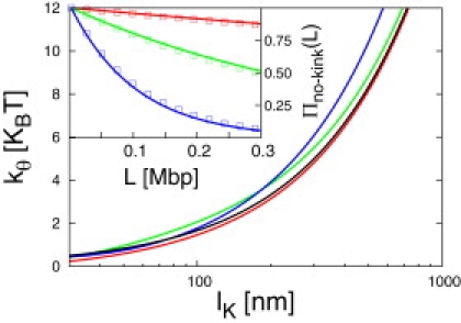
Kuhn length of the fiber as a function of the stiffness constant k_θ (in temperature units) for the three bending potentials, as shown in Eqs. 8–10. (Black line) Large-k_θ analytical expression obtained for potentials from Eqs. 8 and 9 (l_K ≈ 60βk_θ nm). (Inset) The probability Π_no–kink(L) of observing no kink along the contour length L of a chromatin fiber is affected by the choice of the potential modeling the stiffness of the fiber: results from the exact evaluation of Eqs. 11 and 13 (lines) and for simulated fibers after switch among the potentials from Eqs. 8–10 (squares). Colors as in Fig. 3.

Clearly, the values for 〈cos θ〉 (and consequently, l_K) are almost identical between the different potentials. We may therefore switch between the bending potentials, Eqs. 8–10, without affecting the large-scale chain statistics. Obviously, such a switch should entail the appearance and disappearance of the expected, small number of kinks. Using Eq. 11, the probability Π_no–kink(L) of observing no kink along the contour length L is given by

$${\Pi }_{\text{no}-\text{kink}}\left(L\right)={\left(1-\sigma \zeta \right)}^{L/\sigma -1},L>\sigma .$$ (13)

Fig. 4 (inset) shows Π_no–kink(L) as obtained by direct evaluation of Eq. 13 (lines) and for simulated fibers after a switch among the potentials in Eqs. 8–10 (squares). The excellent agreement indicates that our fibers are properly reequilibrated.

Average square internal distances for simulated chromosomes

Given a MD time series with N_t sampled configurations, r_b^ch(i) (b = 1, …, N_b) is the spatial position of the b^th bead from one chosen end of the ch^th chain (ch = 1, …, N_ch) in the i^th configuration (i = 1, …, N_t). Then, the spatial vector connecting chain monomers b and b + l is d_{b, l}^ch(i) = r_b+l^ch(i) − r_b^ch(i). The average square internal distance R^{2, ch}_L between sites separated by l monomers along the ch^th chain is defined as

$$R_{\mathrm{L}=l·\sigma }^{2,\text{ch}}=\frac{1}{N_{\mathrm{t}}\left(N_{\mathrm{b}}-l\right)}\sum _{\mathrm{i}=1}^{N_t}\sum _{\mathrm{b}=1}^{N_b-l}{\left({\mathbf{d}}_{\mathrm{b},\mathrm{l}}^{\text{ch}}\left(i\right)\right)}^2.$$ (14)

The reported average square internal distances R²_L were obtained by averaging Eq. 14 over the complete set of N_ch simulated chains,

$$R_{\mathrm{L}}^2=\frac{1}{N_{\mathit{c}\mathit{h}}}\sum _{\text{ch}=1}^{{\mathrm{N}}_{\text{ch}}}{R}_{\mathrm{L}}^{2,\text{ch}}$$

and corresponding error bars were calculated as the standard deviation from the mean.

Chain looping probabilities for simulated chromosomes

In the same way, we define the spatial distance between monomers b and b + l on the ch^th chain as

$$d_{\mathrm{b},\mathrm{l}}^{\text{ch}}\left(i\right)=\Vert {\mathbf{d}}_{\mathrm{b},\mathrm{l}}^{\text{ch}}\left(i\right)\Vert \text{.}$$

Then, the average looping probability $J_{{\mathrm{L},\mathrm{r}}_{\mathrm{c}}}^{\text{ch}}$ between sites separated by l monomers along the ch^th chain is defined as

$$J_{\mathrm{L}=l·\sigma ,{\mathrm{r}}_{\mathrm{c}}}^{\text{ch}}=\frac{1}{V_{\text{int}}\left(r_{\mathrm{c}}\right)}\frac{1}{N_{\mathrm{t}}\left(N_{\mathrm{b}}-l\right)}\sum _{\mathrm{i}=1}^{{\mathrm{N}}_{\mathrm{t}}}\sum _{\mathrm{b}=1}^{{\mathrm{N}}_{\mathrm{b}}-l}\Theta \left(r_{\mathrm{c}}-d_{\mathrm{b},\mathrm{l}}^{\text{ch}}\left(i\right)\right),$$ (15)

where Θ(x) is the Heaviside step function. The reported looping probabilities $J_{{\mathrm{L},\mathrm{r}}_{\mathrm{c}}}$ were obtained by averaging Eq. 15 over the complete set of N_ch simulated chains,

$$J_{{\mathrm{L},\mathrm{r}}_{\mathrm{c}}}=\frac{1}{N_{\mathit{c}\mathit{h}}}{\sum }_{\text{ch}=1}^{{\mathrm{N}}_{\text{ch}}}{J}_{{\mathrm{L},\mathrm{r}}_{\mathrm{c}}}^{\text{ch}},$$

and corresponding error bars were calculated as the standard deviation from the mean.

3C interaction frequencies X(L) and chain looping probabilities J(L;r_min, r_c)

3C interaction frequencies X(L) and looping probabilities J(L;r_min, r_c) (defined by Eq. 2) are linked by X(L) = κJ(L;r_min, r_c), where κ is a proportionality constant that takes into account the efficiency of the cross-linking reaction (10). Unfortunately, κ is not known. In this work, we have used the normalization

$${\lim }_{\mathrm{L}\to 0}J\left(L;r_{\text{min}},r_{\mathrm{c}}\right)=\frac{1}{V_{\text{int}}}$$

where V_int is the reacting volume (see An Interpolation Formula for Chain Looping). Hence, throughout the text, 3C experimental data have been multiplied by a suitable constant that compensates for the unknown factor κ and thus allows comparison to theoretical predictions.

Results

Wormlike 30-nm fibers

As a first step, we have compared the looping probabilities predicted by our interpolation formula for the end-to-end distance probability density (Eq. 5, together with Eqs. 2 and 3) to the looping probabilities between sites in simulated 30-nm wormlike chromatin fibers with l_K = 300 nm (8,19) and at increasing capture radii r_c (Fig. 5, top). Because our interpolation formula applies to WLCs without kinking, we have used

$$U_{\text{stiff}}\left(\theta \right)=\frac{k_{\theta }}{2}{\theta }^2$$

(Eq. 8) as bending potential. The excellent agreement validates both our theory and the employed simulation/data analysis.

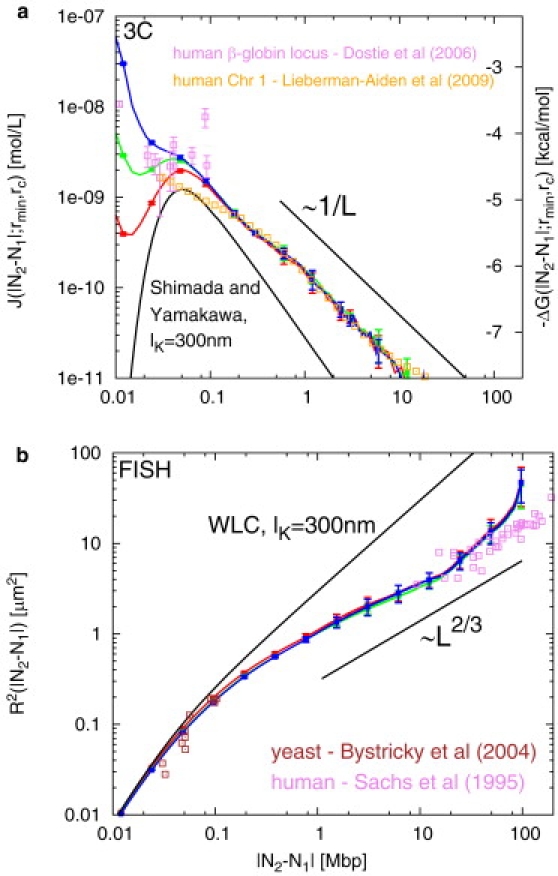
Figure 5.

Looping probabilities J(L;r_min, r_c) between chromatin loci in wormlike 30-nm fibers with l_K = 300 nm (8,19). (Top) Theoretical predictions (solid lines) derived from our interpolation expression for the probability density of internal distances p_L^I(r) (Eq. 5, together with Eqs. 2 and 3) agree with measured looping probabilities (squares) in equilibrated model 30-nm fibers. (Bottom) Experimental 3C interaction frequencies in yeasts (10) may be reproduced only assuming unrealistically high contact radii. Solid lines are the same as in top panel.

In a second step, we have compared the looping probabilities for wormlike chains to experimental data in budding yeasts (in fact, being very small, yeast chromosomes have enough time to mix and equilibrate (19), and therefore represent an interesting case study to test our theory). To account for 3C interaction frequencies in yeasts (10), retaining a fiber Kuhn length l_K = 300 nm, it is necessary to assume unphysically large contact radii (r_c ≳100 nm, Fig. 5, bottom).

In contrast, when reducing the Kuhn length to 56 nm (10), the WLC can account for the data using realistic contact radii (Fig. 6, top). However, this ≈5-times smaller value for the Kuhn length is clearly incompatible with FISH data on internal distances between chromosome sites (Fig. 6, bottom). We can exclude possible effects due to different stages of the cell cycle: both 3C and FISH data were collected in yeast cells during the G₁ phase (8,10). We conclude that the combined experimental evidence on intrachromosomal contacts cannot be accounted-for, on the basis of the WLC model.

Figure 6.

By using a softer chromatin fiber with l_K = 56 nm (3), theoretical predictions for looping probabilities J(L;r_min, r_c) (solid lines) derived from our interpolation expression for the probability density of internal distances p_L^I(r) (Eq. 5, together with Eqs. 2 and 3) reproduce well 3C interaction frequencies in yeasts (10) (top). However, average square internal distances between chromatin sites measured by FISH (8) are clearly off when compared to the theoretical WLC expression from Eq. 1 (bottom).

Kinkable 30-nm fibers

Following a recent discussion in the DNA literature (24,25), it turns out that this apparent paradox can be solved by assuming the presence of a small concentration of kinks along the chromatin fiber.

Fig. 7 (top) shows again the same experimental data, this time in comparison to simulation results for the three different bending potentials (solid lines). In all three cases (and throughout the remainder of this article as well), l_K = 300 nm and we use a physically sensible value of r_c = 45 nm for the contact radius. The effect on the predicted looping probabilities at short genomic distances is dramatic. As few as ≈10 kinks/Mbp increase the contact probabilities in the experimental range by up to ≈2 orders of magnitude and are sufficient to reproduce the observed 3C interaction frequencies in yeasts. At the same time, the predictions of the wormlike and the kinkable chromatin fiber model for FISH experiments are nearly indistinguishable (Fig. 7, bottom). This apparent discrepancy can be understood by comparing the corresponding internal distance probability densities p_L(r) (Fig. S1 in the Supporting Material). The curves have the general features expected for semiflexible chains. In particular, they are peaked at short length-scales and become Gaussian-like at large length-scales. The point to note is that different bending potentials strongly affect the wings of the distribution (r ≤ r_c, vertical lines in Fig. S1) responsible for the 3C signal, but lead to no changes in the peak regions of the distributions that determine the FISH signal (compare the logarithmic scales used in Fig. 7 (bottom) and the linear scales used in Fig. S1). We remark here that the insensitivity of FISH to kinking effects is not a matter of experimental resolution: rather, it should be viewed as an intrinsic limitation on the kind of information that can be effectively extracted from the use of this technique.

Figure 7.

Minimal concentrations of kink along the chromatin fiber increase looping probabilities at short length-scales to up to ≈2 orders of magnitude (top). However, FISH is rather insensitive to kinks (bottom). In both panels, the Kuhn length l_K of the chromatin fiber is = 300 nm. Colors as in Fig. 3.

Chromosome territories and confinement effects

In our previous work, we showed that incomplete relaxation of the bulk of long chromosomes (like in humans and Drosophila) due to topological constraints lead to formation of distinct territories, while telomeric regions can reptate into neighboring territories and equilibrate (19). Fig. 7 (top) also contains looping probabilities between sites located on the tails of model human chromosomes (dashed lines). The same holds for the FISH data: they are almost indistinguishable from predictions of the equilibrated yeast chromosomes (Fig. 7, bottom).

Instead, how do topological constraints influence looping probabilities? Fig. 8 (top) shows looping probabilities between internal sites on model human chromosomes. We immediately observe that, although the short-L behavior reproduces the general patterns previously reported in model yeast chromosomes, the large length-scale behavior is compatible with the power law J(L;r_min, r_c) ∼ L⁻¹, which sharply contrasts the (Gaussian) behavior J(L;r_min, r_c) ∼ L^−3/2 found in equilibrated chromatin fibers (Fig. 7, top). The origin of this discrepancy relies on the different fractal structure of human and yeast chromosomes. In fact, the large-L behavior of the average square internal distances between human chromosome sites follows R²(L) ≈ L^2ν with ν = 1/3 (19). Hence, p_L(r) has to obey the scaling form p_L(r) ≈ L^−3νf(r/L^ν) with f(0) ≠ 0. It is easy to show (see Eq. 2) that, in the large-L limit, J(L;r_min, r_c) ∼ f(0)/L^3ν, which immediately implies J(L;r_min, r_c) ∼ L⁻¹. This characteristic behavior of crumpled-globules (18) is clearly borne out by our simulations data (Fig. 8, bottom).

Figure 8.

(Top) Looping probabilities J(L;r_min, r_c) (left y axis) and looping free energy cost ΔG(L;r_min, r_c) (right y axis) between chromatin sites on model human chromosomes. The large length-scale behavior is compatible with the power law ∼ L⁻¹. (Black line) Shimada and Yamakawa (22) theoretical expression from Eq. 5. (Bottom) In agreement with our finding for model yeast chromosomes (Fig. 7, bottom), FISH is insensitive to kinking. Here, average square internal distances for model human chromosomes have been calculated by assuming the existence of a centromere-hinge, as explained in our previous work (19). Colors as in Fig. 3.

At the time of writing, the experimental test of this prediction seemed far away. However, in the week before the submission of this article, a new, extensive set of Hi-C data appeared (13) (orange squares, Fig. 8) that is in perfect agreement with the predictions from our parameter-free model of interphase chromosomal structure and dynamics. In fact, based on a comparison to simulation data for a related model, Lieberman-Aiden et al. (13) arrives at the same conclusion about the ∼L⁻¹ scaling.

This relation has also an immediate thermodynamical implication. In fact, by defining the corresponding looping free energy cost ΔG(L;r_min, r_c) (expressed in [kcal/mol]) as

$$\Delta G\left(L;r_{\min },r_{\mathrm{c}}\right)=-R_{\text{gas}}T\log \left[J\left(L;r_{\min },r_{\mathrm{c}}\right)\times V_{\text{int}}\right],$$ (16)

where R_gas = 1.987 cal/mol.K is the gas constant and T = 298 K is the room temperature in Kelvin, we deduce that large-L looping inside territories is thermodynamically favored (Fig. 8, top, right y axis) when compared to looping between equilibrated 30-nm fibers of equal contour length (black curve).

For the sake of completeness, we report the average square internal distances between chromosome sites (Fig. 8, bottom panel). In agreement with our previous finding for model yeast chromosomes (Fig. 7, bottom), these curves are insensitive to kinking, as well.

To check the robustness of these findings, we have compared predictions from model human chromosomes to ring polymers of different sizes (see Fig. 9 and Fig. S2). In line with our published results on the internal structure of interphase chromosomes (19) (reproduced in Fig. 9, bottom), looping probabilities also beautifully collapse on a single master curve (Fig. 9, top). As reported in Rosa and Everaers (19), noticeable discrepancies are likely to be simulation artifacts that stem from different choices made in the initial configuration.

Figure 9.

Looping probabilities J(L;r_min, r_c) (top) and average square internal distances (bottom) between chromatin sites on model human chromosomes and ring polymers of different linear sizes collapse to single curves. Here, we have reported simulations results corresponding to the fiber stiffness potential U_stiff(θ) = k_θ(1 − cos θ) from Eq. 9. (Bottom panel, green solid line) Corresponding to the line plotted in Fig. 8, bottom. We remark that noticeable discrepancies between the curves are likely to be simulation artifacts, which are due to different choices in the initial configurations (19).

Conclusions

In this article, we have presented an extended theoretical and computational framework to explain the FISH and 3C data for various species on the basis of a unique, minimal model of decondensing chromosomes: a kinkable, topologically constraint, semiflexible polymer with the (FISH) Kuhn length of l_K = 300 nm, 10 kinks per Mbp, and a contact distance of 45 nm. This provides the basis for the interpretation of the wealth of forthcoming experimental results from new 3C-based technologies (3,11) and the identification of biological functions via a comparison to a well-founded physical reference model.

In particular, we have presented the following results:

We have given a simple, analytical expression for looping probabilities between sites on wormlike chromatin fibers for finite fiber diameter and finite contact radii. This formula is based on the analytical expression recently proposed by us (N. Becker, A. Rosa, and R. Everaers, unpublished) for the end-to-end distance probability density between two sites, which is valid for all fiber stiffnesses and contour lengths, and that generalizes the classical formula by Shimada and Yamakawa (22). Through comparison to 3C interaction frequencies, we have found that the WLC cannot account for all experimental data at the same time (compare Figs. 1 and 2).

In line with recent modeling effort to explain unexpectedly high cyclization probabilities of short DNA fragments (24,25), we have shown that one can expect strong enhancement of contacts between sites located at genomic distances smaller than the chromatin Kuhn length of ≈0.03 Mbp if the fiber presents local curvature defects (kinks). In particular, good agreement with 3C experimental data is found by assuming the very small density of ≈10 kinks/Mbp, corresponding to an energy penalty of ≈10 k_BT to kink a short chromatin fragment between two nucleosome core particles (37).

Topological constraints confine the bulk of long chromosomes (like in humans) to distinct territories (19), which can then be described as crumpled-globules (18). This implies that the large-scale fractal behavior of the average-square internal distances between marked chromatin sites is given by R²(L) ∼ L^2/3, in sharp contrast with the Gaussian behavior R²(L) ∼ L found for short equilibrated chromosomes (like in yeasts). In turn, this implies that whereas contact probabilities between distant sites in yeasts decay like ∼L^−3/2, the large-scale interaction frequencies between sites on long chromatin fibers decay like ∼L⁻¹ (see Chromosome Territories and Confinement Effects), a prediction that has very recently received experimental confirmation (13).

An interesting corollary from our previous work is the necessity to distinguish between the behavior of the bulk of a long chromosome and its telomeric region. The latter can equilibrate by randomly extending into and retracting from neighboring territories. For example, we argued that the FISH data for the terminal 4p16.3 region reported in Sachs et al. (7) should be atypical for the chromosome as a whole. By the same logic, we expect that intrachain contacts in the terminal region should be suppressed relative to the bulk of the chromosome, while the generic model suggests the opposite trend for interchain interactions.

Finally, we note that in this work we have assumed that interphase chromosomes form 30-nm diameter chromatin fibers with local defects represented via generic kinks. There is evidence that interphase chromosomes (partially) behave like solutions of disordered 10-nm diameter fibers (39). This would not invalidate our kinetic arguments for the existence of territories, as a stronger decondensation would not change the topological state of the fiber (with respect to entanglements) or lead to a faster equilibration. We leave the investigation of this scenario and of the possibility of a simultaneous presence of condensed and decondensed chromosome regions for future work.

Appendix

Equation 5 contains the following expressions and numerical constants (23),

$$\begin{array}{c}\rho =r/L\\ \lambda =l_{\mathrm{K}}/2L\\ a=14.054\\ b=0.473\\ c_{\text{ij}}=\left(\begin{array}{ccc}-3/4& 23/64& -7/64\\ -1/2& 17/16& -9/16\end{array}\right)\\ 1-c={\left(1+{\left(0.38{\lambda }^{-0.95}\right)}^{-5}\right)}^{-1/5}\\ 1-d=\{\begin{array}{cc}0& \lambda <1/8\\ \frac{1}{0.177/\left(\lambda -0.111\right)+6.40{\left(\lambda -0.111\right)}^{0.783}}& \text{otherwise},\end{array}\end{array}$$

and I₀(x) is a modified Bessel function of the first kind. J_SY(L) is the so-called Shimada and Yamakawa J-factor, which measures the ring closure probability at any orientation of chain ends (J_SY (L) = lim_r→0 J(L;0,r) = p_L(0), Eq. 2). It is given by a closed interpolation formula that matches between the short (L ≲ l_K) and large (L ≫ l_K) exact length-scale behaviors of a WLC (22). For the sake of completeness, we report also the complete expression for J_SY(L) (Eqs. 50 and 65 in Shimada and Yamakawa (22)):

$$J_{\text{SY}}\left(L\right)=\frac{1}{l_{\mathrm{K}}^3}\times \{\begin{array}{ll}896.32{\lambda }^5\exp \left(-14.054\lambda +\frac{0.246}{\lambda }\right),\hfill & \lambda \ge 8\hfill \\ {\left(\frac{3\lambda }{\pi }\right)}^{3/2}\left(1.0-\frac{5\lambda }{4}-\frac{79{\lambda }^2}{160}\right),\hfill & \text{otherwise}.\hfill \end{array}$$

Other recent works of relevance to this article include Cook and Marenduzzo (40) and Dorier and Stasiak (41).

Supporting Material

Two figures are available at http://www.biophysj.org/biophysj/supplemental/S0006-3495(10)00219-5.

References

- 1.Aten J.A., Kanaar R. Chromosomal organization: mingling with the neighbors. PLoS Biol. 2006;4:e155. doi: 10.1371/journal.pbio.0040155. [DOI] [PMC free article] [PubMed] [Google Scholar]
- 2.Cremer T., Cremer C. Chromosome territories, nuclear architecture and gene regulation in mammalian cells. Nat. Rev. Genet. 2001;2:292–301. doi: 10.1038/35066075. [DOI] [PubMed] [Google Scholar]
- 3.Dekker J. Gene regulation in the third dimension. Science. 2008;319:1793–1794. doi: 10.1126/science.1152850. [DOI] [PMC free article] [PubMed] [Google Scholar]
- 4.Cavalli G. Chromosome kissing. Curr. Opin. Genet. Dev. 2007;17:443–450. doi: 10.1016/j.gde.2007.08.013. [DOI] [PubMed] [Google Scholar]
- 5.Vernimmen D., De Gobbi M., Higgs D.R. Long-range chromosomal interactions regulate the timing of the transition between poised and active gene expression. EMBO J. 2007;26:2041–2051. doi: 10.1038/sj.emboj.7601654. [DOI] [PMC free article] [PubMed] [Google Scholar]
- 6.Lomvardas S., Barnea G., Axel R. Interchromosomal interactions and olfactory receptor choice. Cell. 2006;126:403–413. doi: 10.1016/j.cell.2006.06.035. [DOI] [PubMed] [Google Scholar]
- 7.Sachs R.K., van den Engh G., Hearst J.E. A random-walk/giant-loop model for interphase chromosomes. Proc. Natl. Acad. Sci. USA. 1995;92:2710–2714. doi: 10.1073/pnas.92.7.2710. [DOI] [PMC free article] [PubMed] [Google Scholar]
- 8.Bystricky K., Heun P., Gasser S.M. Long-range compaction and flexibility of interphase chromatin in budding yeast analyzed by high-resolution imaging techniques. Proc. Natl. Acad. Sci. USA. 2004;101:16495–16500. doi: 10.1073/pnas.0402766101. [DOI] [PMC free article] [PubMed] [Google Scholar]
- 9.Branco M.R., Pombo A. Intermingling of chromosome territories in interphase suggests role in translocations and transcription-dependent associations. PLoS Biol. 2006;4:e138. doi: 10.1371/journal.pbio.0040138. [DOI] [PMC free article] [PubMed] [Google Scholar]
- 10.Dekker J., Rippe K., Kleckner N. Capturing chromosome conformation. Science. 2002;295:1306–1311. doi: 10.1126/science.1067799. [DOI] [PubMed] [Google Scholar]
- 11.Simonis M., Kooren J., de Laat W. An evaluation of 3C-based methods to capture DNA interactions. Nat. Methods. 2007;4:895–901. doi: 10.1038/nmeth1114. [DOI] [PubMed] [Google Scholar]
- 12.Dostie J., Richmond T.A., Dekker J. Chromosome conformation capture carbon copy (5C): a massively parallel solution for mapping interactions between genomic elements. Genome Res. 2006;16:1299–1309. doi: 10.1101/gr.5571506. [DOI] [PMC free article] [PubMed] [Google Scholar]
- 13.Lieberman-Aiden E., van Berkum N.L., Dekker J. Comprehensive mapping of long-range interactions reveals folding principles of the human genome. Science. 2009;326:289–293. doi: 10.1126/science.1181369. [DOI] [PMC free article] [PubMed] [Google Scholar]
- 14.Bystricky K., Laroche T., Gasser S.M. Chromosome looping in yeast: telomere pairing and coordinated movement reflect anchoring efficiency and territorial organization. J. Cell Biol. 2005;168:375–387. doi: 10.1083/jcb.200409091. [DOI] [PMC free article] [PubMed] [Google Scholar]
- 15.Münkel C., Langowski J. Chromosome structure predicted by a polymer model. Phys. Rev. E Stat. Phys. Plasmas Fluids Relat. Interdiscip. Topics. 1998;57:5888. [Google Scholar]
- 16.Bohn M., Heermann D.W., van Driel R. Random loop model for long polymers. Phys. Rev. E Stat. Nonlin. Soft Matter Phys. 2007;76:051805. doi: 10.1103/PhysRevE.76.051805. [DOI] [PubMed] [Google Scholar]
- 17.Nicodemi M., Prisco A. Thermodynamic pathways to genome spatial organization in the cell nucleus. Biophys. J. 2009;96:2168–2177. doi: 10.1016/j.bpj.2008.12.3919. [DOI] [PMC free article] [PubMed] [Google Scholar]
- 18.Grosberg A., Rabin Y., Neer A. Crumpled globule model of the three-dimensional structure of DNA. Europhys. Lett. 1993;23:373. [Google Scholar]
- 19.Rosa A., Everaers R. Structure and dynamics of interphase chromosomes. PLoS Comput. Biol. 2008;4:e1000153. doi: 10.1371/journal.pcbi.1000153. [DOI] [PMC free article] [PubMed] [Google Scholar]
- 20.Rippe K. Making contacts on a nucleic acid polymer. Trends Biochem. Sci. 2001;26:733–740. doi: 10.1016/s0968-0004(01)01978-8. [DOI] [PubMed] [Google Scholar]
- 21.Douarche N., Cocco S. Protein-mediated DNA loops: effects of protein bridge size and kinks. Phys. Rev. E Stat. Nonlin. Soft Matter Phys. 2005;72:061902. doi: 10.1103/PhysRevE.72.061902. [DOI] [PubMed] [Google Scholar]
- 22.Shimada J., Yamakawa H. Ring-closure probabilities for twisted wormlike chains. Application to DNA. Macromolecules. 1984;17:689. [Google Scholar]
- 23.Reference deleted in proof.
- 24.Wiggins P.A., Phillips R., Nelson P.C. Exact theory of kinkable elastic polymers. Phys. Rev. E Stat. Nonlin. Soft Matter Phys. 2005;71:021909. doi: 10.1103/PhysRevE.71.021909. [DOI] [PMC free article] [PubMed] [Google Scholar]
- 25.Yan J., Kawamura R., Marko J.F. Statistics of loop formation along double helix DNAs. Phys. Rev. E Stat. Nonlin. Soft Matter Phys. 2005;71:061905. doi: 10.1103/PhysRevE.71.061905. [DOI] [PubMed] [Google Scholar]
- 26.Finch J.T., Klug A. Solenoidal model for superstructure in chromatin. Proc. Natl. Acad. Sci. USA. 1976;73:1897–1901. doi: 10.1073/pnas.73.6.1897. [DOI] [PMC free article] [PubMed] [Google Scholar]
- 27.Doi M., Edwards S.F. Oxford University Press; New York: 1986. The Theory of Polymer Dynamics. [Google Scholar]
- 28.Rubinstein M., Colby R.H. Oxford University Press; New York: 2003. Polymer Physics. [Google Scholar]
- 29.Wilhelm J., Frey E. Radial distribution function of semiflexible polymers. Phys. Rev. Lett. 1996;77:2581–2584. doi: 10.1103/PhysRevLett.77.2581. [DOI] [PubMed] [Google Scholar]
- 30.Thirumalai D., Ha B.Y. Academic Press; San Diego CA: 1998. Statistical Mechanics of Semiflexible Chains: a Mean-Field Variational Approach. [Google Scholar]
- 31.Winkler R.G. Deformation of semiflexible chains. J. Chem. Phys. 2003;118:2919. [Google Scholar]
- 32.Mehraeen S., Sudhanshu B., Spakowitz A.J. End-to-end distribution for a wormlike chain in arbitrary dimensions. Phys. Rev. E Stat. Nonlin. Soft Matter Phys. 2008;77:061803. doi: 10.1103/PhysRevE.77.061803. [DOI] [PubMed] [Google Scholar]
- 33.Lee K., Kang M.J., Kwon H. Expansion of chromosome territories with chromatin decompaction in BAF53-depleted interphase cells. Mol. Biol. Cell. 2007;18:4013–4023. doi: 10.1091/mbc.E07-05-0437. [DOI] [PMC free article] [PubMed] [Google Scholar]
- 34.Kremer K., Grest G.S. Dynamics of entangled linear polymer melts: a molecular-dynamics simulation. J. Chem. Phys. 1990;92:5057. [Google Scholar]
- 35.Worcel A., Strogatz S., Riley D. Structure of chromatin and the linking number of DNA. Proc. Natl. Acad. Sci. USA. 1981;78:1461–1465. doi: 10.1073/pnas.78.3.1461. [DOI] [PMC free article] [PubMed] [Google Scholar]
- 36.Lankas F., Lavery R., Maddocks J.H. Kinking occurs during molecular dynamics simulations of small DNA minicircles. Structure. 2006;14:1527–1534. doi: 10.1016/j.str.2006.08.004. [DOI] [PubMed] [Google Scholar]
- 37.Mergell B., Everaers R., Schiessel H. Nucleosome interactions in chromatin: fiber stiffening and hairpin formation. Phys. Rev. E Stat. Nonlin. Soft Matter Phys. 2004;70:011915. doi: 10.1103/PhysRevE.70.011915. [DOI] [PubMed] [Google Scholar]
- 38.Alberts B., Johnson A., Walter P. Garland Science; New York: 2002. Molecular Biology of the Cell. [Google Scholar]
- 39.Dehghani H., Dellaire G., Bazett-Jones D.P. Organization of chromatin in the interphase mammalian cell. Micron. 2005;36:95–108. doi: 10.1016/j.micron.2004.10.003. [DOI] [PubMed] [Google Scholar]
- 40.Cook P.R., Marenduzzo D. Entropic organization of interphase chromosomes. J. Cell Biol. 2009;186:825–834. doi: 10.1083/jcb.200903083. [DOI] [PMC free article] [PubMed] [Google Scholar]
- 41.Dorier J., Stasiak A. Topological origins of chromosomal territories. Nucleic Acids Res. 2009;37:6316–6322. doi: 10.1093/nar/gkp702. [DOI] [PMC free article] [PubMed] [Google Scholar]
Associated Data
This section collects any data citations, data availability statements, or supplementary materials included in this article.