Quantification of Clustering in Joint Interspike Interval Scattergrams of Spike Trains

Abstract

Joint interval scattergrams are usually employed in determining serial correlations between events of spike trains. However, any inherent structures in such scattergrams that are often seen in experimental records are not quantifiable by serial correlation coefficients. Here, we develop a method to quantify clustered structures in any two-dimensional scattergram of pairs of interspike intervals. The method gives a cluster coefficient as well as clustering density function that could be used to quantify clustering in scattergrams obtained from first- or higher-order interval return maps of single spike trains, or interspike interval pairs drawn from simultaneously recorded spike trains. The method is illustrated using numerical spike trains as well as in vitro pairwise recordings of rat striatal tonically active neurons.

Introduction

Neuronal spike-train sequences often exhibit an underlying correlation structure despite their interspike interval (ISI) variability (1–4). A common method of visualizing the underlying structures is the use of joint ISI scattergrams. For a single spike train, a joint ISI scattergram is constructed by computing the first-order return maps (which plot the given ISI sequence α_i versus its time-lagged sequence α_i+1), which pictorially depict geometric dependence between the neighboring ISIs (5,6). For visualizing dependencies between higher-order neighbors, higher-order return maps can be constructed using longer time lags between the ISIs. The scattergrams are not limited to single spike-train sequences, but can be extended to pairs of simultaneously recorded spike trains. For such pairs of spike trains, pairs of ISIs at any given time instance may be obtained by interpreting the sequence of ISIs as a sequence of states of the neuron (7), and scattergrams of the state pairs can be constructed. Another method of visualizing simultaneous spike trains is to construct joint peristimulus time histograms (8), which again offer a visual depiction of inherent structures between instantaneous rates derived from the ISIs.

A commonly used method to quantify joint ISI scattergrams is computing a serial or Pearson correlation coefficient. The serial correlation coefficient can be a sufficient description of a datum that is void of any dominant inherent structure. However, a considerable amount of crowding and structure between the interval pairs can be seen in some experimental return maps (2,6,9–12). These structures are the density modulations of the ISI pairs within the scattergrams. A serial correlation coefficient fails to quantify these structures, because the coefficient simply measures the degree of association between pairs, and does not attempt to parse the structures.

Another method that has been employed to quantify the ISI scatter is the so-called box dimension borrowed from nonlinear time series analysis techniques. This method has been applied to single spike-train sequences (13–16), as well as to scattergrams, to estimate the dimensionality of the attractors (6) caused by the ISI pairs, and it thus may provide a quantification of the scatter among the ISI pairs. A box dimension for a scattergram requires that square boxes of fixed sizes be constructed in the two-dimensional space. The number of such boxes with one or more ISI pairs is taken into account. The exponent of that number as a function of the side length of the boxes results in the box dimension. This measure does not account for the density in each such square. For example, if all the pairs under observation fall in a single box, then the box dimension would become zero, and if the ISI pairs are uniformly scattered in the two-dimensional plane, then it would tend to 2. Thus, this method computes the dimensional spread of the underlying data pairs, and not the density observed in the scattergrams.

Here, we describe a hierarchical method that directly quantifies the density modulations observed in a given scattergram. We introduce a cluster coefficient that is proportional to the local number density of pairs of points in the scattergrams. A profile of such cluster coefficients is obtained systematically as a function of the scale length in the scattergram. In addition, a clustering density is defined by taking the derivative of the cluster coefficient profile. The clustering density is amenable for computing statistical quantities such as first- and second-order moments that quantify the deviations in clustering in the space of lengthscale of the scattergram.

The modulations in a scattergram result in local crowding. Crowding of ISI pairs can naturally arise in experiments due to temporal clustering of spike events (1,17,18). However, not all clusters of points in the joint scattergrams are caused by temporal clustering of intervals. For our purposes, a cluster is viewed as a group of points (i.e., ISI pairs) in a fixed rectangle in the scattergram, and every pair in the scattergram falls in a cluster. The total rectangular area of the scattergram is split into a fixed number of smaller rectangular boxes, and the group of pairs in each rectangular box is referred to as a cluster. The cluster coefficient is proportional to the weighted sum of the number densities in the rectangular boxes. A cluster coefficient of unity would correspond to the case of all the pairs falling in a single rectangle, and is smaller in the case where pairs span more than one rectangle. The spacing of the rectangular grid is an adjustable parameter that depends on the mean values of the intervals along each axis. A cluster coefficient is computed at each level of the grid spacing, and thus, a functional profile of the coefficient is obtained that reveals the clustering at different lengthscales. We formulate the method and define the cluster coefficient and the clustering density in the next section. The method is applied then to spike-train sequences obtained from a stochastic FitzHugh-Nagumo neuron model with different noise levels, as well as to spike-train pairs obtained from pairwise recordings of rat striatal neurons in slices.

Cluster Coefficient and Clustering Density

The cluster coefficient is defined based on the two-dimensional density of the scattergrams. We illustrate the construction of pairs of ISIs from a pair of spike-train sequences. The ISI pairs are represented in a two-dimensional phase plane whose sides represent ISI sequences derived from the spike trains. Fig. 1, a and b, illustrates first return maps (serial correlograms) of ISIs obtained from two simultaneously recorded, tonically active striatal neurons plotted individually under control conditions, and Fig. 1 e shows the scattergram between the two cells obtained from forming pairs according to the methods of Kreuz et al. (7). Fig. 1, c–f, represents the corresponding scattergrams with apamin applied to the bath. Application of the drug alters the scattergram distribution of ISI pairs, in some cases reducing the size of the dominant single cluster. To quantify the clustering, a rectangular grid is formed in which the grid spacing along either axis is proportional to the mean ISI of the spike-train sequence represented on the corresponding axis. The number of ISI pairs in each nonempty rectangular bin is computed and a cluster coefficient is defined on them.

Figure 1.

Typical scattergrams quantified by cluster coefficient C_w and clustering density F(w). (a–d) Cumulative joint ISI scattergrams (from across all the experimental trials) of two tonically active striatal neurons under control (a and b) and under application of apamin (c and d). These scattergrams plot first return maps (ISI_n versus ISI_n+1) of the recorded ISI sequences. (e and f) Mutual ISI pairs formed from the two simultaneous recordings under the two conditions. (g and h) The ISI densities under the two conditions for cell 1 (g) and cell 2 (h) are displayed. This example is analyzed in the Applications section.

Computing ISI pairs

Pairs from a single spike train

Let A_i, i = 1, …, N_A be the given spike-train sequence. The ISI pair sequence is obtained from return maps of the ISIs. The first-order return maps are obtained by forming pairs from the sequence A_i and its time-lagged sequence A_i+1. The ISI pairs thus are written as (α_i, β_i) = (A_i+1 − A_i, A_i+2 − A_i+1), where i = 1, …, N_A − 2. These pairs are plotted in the ISI phase plane (α(t), β(t)) for binning the pairs in rectangular intervals. Higher-order return maps are similarly constructed. A kth order sequence of pairs is written as (α_i, β_i) = (A_i+1 – A_i, A_i+k+1 – A_i+k), where i = 1, …, N_A − k − 1.

Pairs from two different spike trains

Let A_i, i = 1, …, N_A, and B_i, i = 1, …, N_B be two spike time sequences for which the cluster coefficient is being sought. Let sequences I_i, i = 1, …, N_A − 1, and J_i, i = 1, …, N_B – 1 be the two ISI sequences derived from the original spike trains. We aim to form pairs of ISIs that would be represented in a two-dimensional plane. I_i and J_i cannot by themselves form pairs of values, because the relative phases at which the spike times of the first cell occur with respect to the spike times of the second cell, and vice versa, do not in general remain constant throughout the length of recording times. However, at any given point of time t, one can readily identify the preceding and succeeding spike times from each spike-train sequence. In other words, each ISI could be thought of as a state of the neuron, and such states could become pairs of values at any point in time, t, or at times corresponding to the spike times of each neuron. This concept was originally described by Kreuz et al. (7), who employed it in defining an ISI-distance measure. Here, (α(t), β(t)) are the ISI pairs constructed according to this concept. α(t) = A_j+1 − A_j, such that A_j ≤ t < A_j+1. In a similar way, β(t) = B_k+1 − B_k, such that B_k ≤ t < B_k+1. Time t either can assume a sequence of times separated by a fixed width or can be discrete, assuming all the values of A_i and B_i. We adopt the latter method here, writing the ISI pairs as (α_i, β_i), i = 1, …, N, where N ≤ N_A + N_B − 2. These ISI pairs are represented as points in a two-dimensional phase plane (α, β).

Defining the cluster coefficient, C_w, from the ISI pairs

We define a cluster as the group of ISI pairs (α_i, β_i) falling in fixed predefined ranges of ISIs. The size of the cluster is the number of such ISI pairs, and the total number of clusters accounts for all ISI pairs. We define a cluster coefficient, C_w, that quantifies the amount of clustering by first identifying groups of ISI pairs (α_i, β_i), arranging them in descending order of size, and then adding the contributions of each group.

Our approach here is to quantify the clustering without using any parameters. However, we do use a scale parameter, w, that determines the size of the rectangular grid for the purpose of finding clusters. We make C_w assume a maximum value in the simple case of a pair of regular spike trains with any frequency, since such a case will simply be a single point with high density in the phase space of ISIs. Two spike train sequences whose spike times are phase-locked in a 1:2 ratio will show two clusters in the ISI phase space described earlier, but will possess a cluster coefficient less than unity.

The given spike train sequences A_i and B_i are converted to interspike interval pairs (α_i, β_i), i = 1, …, N, as described earlier. N is the total number of ISI pairs. Let $\langle \alpha \rangle =\frac{1}{N}\sum _{i=1}^N{\alpha }_i$ and $\langle \beta \rangle =\frac{1}{N}\sum _{i=1}^N{\beta }_i$ be the average ISI values of the two sequences. The ISI pairs are now assigned to two-dimensional rectangular bins of length w〈α〉 along the x axis and w〈β〉 along the y axis. w is a nonnegative constant that determines the bin widths. The ISI pairs falling in each rectangle constitute a cluster. We are not concerned with the distribution of the ISIs within the cluster or the distances between such clusters. Let S_i,_j denote the bin ij that includes all the ISI pairs that fall in the rectangular window [x₀ + w〈α〉(i − 1), x₀ + w〈α〉i] and [y₀ + w〈β〉(j − 1), y₀ + w〈β〉j]. That is, the bin S_ij counts all ISI values for which x₀ + w〈α〉(i − 1) ≤ α_i < x₀ + w〈α〉i and y₀ + w〈β〉(j − 1) ≤β_j < y₀ + w〈β〉j. The values x₀ and y₀ are adjusted such that the biggest density cluster is at the center of the rectangle surrounding it. However, computation of the coordinates of the biggest density cluster itself is carried out by setting x₀ = min{α_i, i = 1, …, N}, and y₀ = min{β_i, i = 1, …, N} and adjusting a grid reference scale length, w = w^ref. The ensuing fluctuations in the computation are discussed later. The bins S_ij are then arranged in descending order of bin counts. Let n_i, i = 1, …, N_C be such an ordered sequence of nonzero bin counts. N_C is the number of nonzero clusters. We call n_i the cluster size of cluster i. The hierarchical nature of n_i as a function of i is illustrated in Fig. 2 a at different w using a scattergram obtained from the stochastic FitzHugh-Nagumo model with noise level D = 0.1. At large w (w = 0.2), there remains only one cluster, and at very small w, equal-sized but small clusters remain.

Figure 2.

Validation of the conditions for cluster coefficient formulation. (a) Number of ISI pairs (n_i) versus i for an ISI scattergram shown of Fig. 3 at different scales, w. At very large w (0.2, for example), there is only one cluster. At w ≈ 0, small clusters (∼1/N) of equal size appear. (b) Using the same scattergram, the coefficients T_i versus w are shown for three values of i. The hierarchical ordering of the clusters ensures that largest clusters (f₁, for example) have larger coefficients (T₂). (c) A cluster coefficient at a w where there is only one big cluster of density d in the scattergram is shown for two different formulations. (d) C_w as a function of the largest density cluster for two scattergrams. (e) Graphical depiction of the area terms that contribute to C_w. The sum of the terms will always be less than or equal to unity. To illustrate, f₁ = 0.5, f₂ = 0.3, and f₃ = 0.15. More clusters will add smaller areas, but will fit within the unit square. (f) Relation between cluster coefficient and number of clusters, N_C, in the case where all clusters have the same cluster size. At large N_C, C_w is inversely proportional to the number of clusters.

Let the local number density be defined by f_i = n_i/N. By definition, f_i ≤ 1, and since the number densities are ordered according to their magnitude, if i > j, then f_i ≤ f_j. Then, the cluster coefficient, C_w, is defined as

$$C_w=f_1+a_2{f}_2+a_3{f}_3+\dots +a_N{f}_N\text{.}$$ (1)

The ratio of the coefficients T_i = a_i/a_i-1 is chosen such that it does not increase with increasing i, and a₁ = 1. Our choice of T_i is guided by the following considerations. We relate C_w to the density of the clusters. Thus, at a value of w for which there remains only one cluster, only the first term f₁ becomes nonzero, and C_w thus becomes unity. If, at a given w, there still remains only one dominant cluster, with all other scattergram points homogeneously distributed, then we want C_w to directly represent this scenario such that f₁ is the biggest contributor to C_w. T_i can become unity for some values of i, but obviously it cannot be unity for all i, because that would render C_w = 1 for all w, and thus make C_w independent of w. The weights a_i are chosen to satisfy three conditions: 1), weight a_i reflects the hierarchy of the local number density, f_i, such that T_i < 1, for i > 1; 2), the dominant factor contributing to C_w is linear in the highest local number density, i.e., f₁; and 3), C_w is a function of w, and is less than or equal to unity for any configuration of f_i values.

Hypothesis: The recursive relation T_i = f_i−1 satisfies the above three conditions.

Fig. 2 b illustrates a scattergram of the stochastic FitzHugh-Nagumo model in which T_i is computed as a function of w. Only T₂ can go up to 1 for large w; all other T_i values are less than or equal to T₂, since they are obtained from terms that have T₂ as a factor. T₂ can increase to 1, because as w increases, the density of the largest cluster increases to unity, and the size of the other clusters must become smaller. Thus, T_i, i = 3, …, N becomes 0 when T₂ approaches unity. The nature of the approach to unity is dependent on the distribution of the ISI pairs in a given scattergram. If the scattergram consists of only one dominant crowded region, then an S-shaped profile toward unity can be expected.

It is easy to validate condition 1. For w = w^∗, let there be two clusters. Then, C_w = f₁ + a₂f₂. However, T₂ = a₂ = f₁ = 1 − f₂ < 1, and the ith coefficient ratio in an N-cluster scattergram is T_i = f_i−1 < 1 by definition. The linearity condition is demonstrated by two examples. Consider again the case of two clusters at w = w^∗. Then,

$$C_w=f_1+a_2{f}_2=f_1+f_1\times \left(1-f_1\right)=2f_1-f_1^2=2d-d^2,$$

where d ≡ f₁ is the density of the largest local cluster. Since d < 1, the second term is much smaller than the first, and consequently, the dominant contribution of the largest local number density, f₁, to C_w is the first power of f₁. As a second example, consider a case where there is only one dense cluster, and the rest of the ISIs are distributed uniformly such that the densities are given by f₁ = d and f_i = 1/N for i = 2, …, N. We assume that there is at least one cluster such that d ranges from 0 to 1 − 1/N. Then, C_w is given by a function that depends on both d and N:

$$\begin{array}{c}{F}_N\left(d\right)=d+a_2\frac{1}{N}+\dots +a_N\frac{1}{N}\\ =d\left(1+\frac{1}{N}+\frac{1}{N^2}+\dots +\frac{1}{N^{N-1}}\right)\\ =d\left(\frac{1-x^N}{1-x}\right)\to d,\text{as}N\to \mathrm{\infty }\end{array},$$ (2)

where x =1/N. This expression is plotted in Fig. 2 c for two values of N. As can be seen directly from this expression, F_N(d) tends to d, the density itself, as N → ∞. We can contrast this property with other possible nonlinear formulations of C_w. If, instead of Eq. 1, we had used a formulation such as ${{\sum }_{i=1}^N{f}_i}^2$ to represent C_w, the above sample scattergram would give the cluster coefficient

$$G_N\left(d\right)=d^2+\frac{1}{N^2}+\dots +\frac{1}{N^2}\text{.}$$ (3)

Thus, the cluster coefficient would become a nonlinear function of d. G_N(d) is illustrated in Fig. 2 c for two values of N. The advantage of a hierarchical choice of coefficients is also evident here. In the nonlinear formulation, the coefficients are not self-determined, and thus, for small N, they need to be corrected to avoid the finite jump in G_N(d), as seen in the figure, when the density itself is close to 0. In our hierarchical choice of coefficients, this is self-corrected, and there is no jump seen in F_N(d) when d = 0. In real scattergrams, however, density distributions among the clusters can be more complex. Fig. 2 d shows the dependence of C_w on the density of the largest cluster, f₁. The value of w is varied to effect changes in f₁ so that it can range between 0 and 1. The value of w at which f₁ reaches unity is different for the results shown in the figure. However, the profile itself is close to linearity. The contribution of other larger clusters becomes significant when considerable deviation from the linearity is seen. The sudden increment seen in the experimental curve for intermediate w is due to the readjustment of the ISI pairs into bigger clusters when w is increased. This can happen because the position of our grid is taken with respect to one biggest cluster at a given w^ref.

To validate the third condition, we first depict geometrically (Fig. 2 e) the areas represented by the terms in the definition of C_w in Eq. 1 as subareas in a unit square. Since each f_i is less than or equal to unity, any product of any number of such terms will also be less than or equal to unity. Also, the sum of all the f_is is equal to unity. The first term, f₁, which represents the biggest density in the hierarchy, is shown by the rectangular area with sides 1 and f₁. The second term, f₁ × f₂, contributes a smaller area than that of the first. Thus, successive terms contribute successively smaller areas, but all terms fit within the unit square whose area is unity. Thus, C_w will always be less than or equal to unity for any configuration of f_is. As an example, we next consider an extreme example in which all clusters are of equal size, which would produce a maximum C_w. For a value of w that results in a single cluster in the scattergram, C_w = 1, but if two or more clusters result, then C_w < 1. We see that for two equal-sized clusters, f₁ = f₂ = ½, which leads to C_w = 0.75. For three equal-sized clusters, f_i = 1/3, i = 1, 2, 3, which leads to C_w = 0.48. For N_C (N/n) clusters of each size n, we have $f_1=\dots =f_{N_C}=f=1/N_C$. Then, the cluster coefficient is given by the expression

$$C_w=f+f^2+\dots +f^{N_C}=\frac{f-f^{N_C+1}}{1-f},$$ (4)

which is valid for all positive integers of N_C. This expression is plotted in Fig. 2 f as a function of the number of clusters (dots are the evaluations at integer values, and the dashed curve is a continuous plot of the expression). For a large number of clusters, C_w is proportional to the inverse of the number of clusters. That is, for a homogeneous and continuous distribution of ISI pairs in the two-dimensional plane, the cluster coefficient becomes equal to the density of the distribution (1/N). We can use this formula to find C_w in the limit of w → 0. In this limit, N_C = N, and thus, f = 1/N and can be assumed to be much smaller than unity for large N. Thus, 1/(1 − f) can be expanded in a Taylor series, and after simplification, we find that to the first order in f, C_w → f = 1/N, which at large N_C validates the result in Fig. 2 f.

The cluster coefficient, C_w, quantifies the clustering between the interval sequences at each value of w. The functional dependence of C_w on w is obtained by increasing w from 0 to a value at which a single rectangle contains all the ISI pairs, and thus a single cluster is formed. Increasing w further has no effect on C_w. For a regular spike train with no ISI deviation, C_w is nothing but a Heaviside function, and for all other types of ISI sequence, C_w always has a profile as a function of w.

Clustering density, F(w)

The growth rate of C_w with respect to w quantifies the density of the hierarchically ordered local number densities. We call this rate the clustering density,

$$F\left(w\right)=\frac{d{C}_w}{dw}\text{.}$$ (5)

F(w) has the characteristics of a density distribution, since its integral is continuous and goes from 0 to 1. Thus, C_w has the characteristics of a cumulative distribution. However, F(w) itself is not a measure of the density of clusters in the scattergram, as we did not consider the mutual distances between the clusters in formulating Cw. F(w) quantifies the rate of change of the clusters, and its coefficient of variation (CV) is a measure of the deviation in the clusters. For a scattergram with a single point (from a regular spike train), C_w becomes a step function with the step at w = 0, and the corresponding F(w) is a delta function with width 0. The width of F(w) becomes nonzero as the scatter of the ISI pairs becomes larger. For the uniform distribution of ISI pairs discussed earlier, the local density at a given w can be written as f_i = f for all i, and f = (w〈ISI〉/Δ)², where Δ is the width of the ISI scatter along any of the axes. The corresponding C_w values (using the formula in Eq. 4), along with results obtained from actual simulations, are presented in Fig. 3 a. The overestimation at large w is caused by the fact that the computational grid is positioned with respect to the highest density point, resulting in f_i < f₁ for i > 2. The mean C_w is smoothed, and its derivative is presented as F(w) in Fig. 3 b. C_w is affected by the rate of the ISIs, but the CV of F(w) is not.

Figure 3.

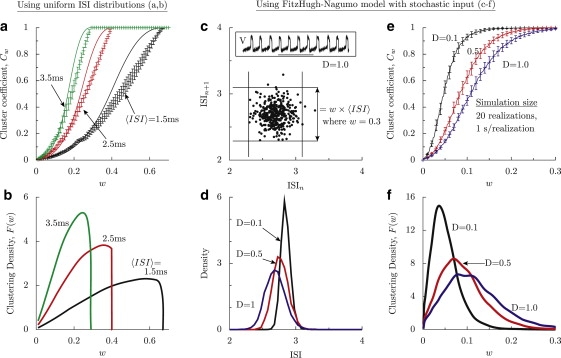
Application of the model to numerical spike trains of uniform ISI distribution (a and b) and the stochastic FitzHugh-Nagumo model (c–f). (a) Cluster coefficient for scattergrams of uniform ISI distributions for three different mean ISIs, keeping the distribution width, Δ, constant at 1 ms. Twenty realizations of 1-s duration were used. The length of the error bars is twice the standard deviation. For computation, the maximum density point of the scattergram is explicitly given as (〈ISI〉, 〈ISI〉), instead of using a w^ref. The solid lines are analytical curves predicted by Eq. 4, with f = (w × 〈ISI〉/Δ)². (b) Clustering density for the corresponding curves in a. The CV of F(w) is unchanged at 0.37 with rate, whereas the CVs of the ISI distribution for 〈ISI〉 = 1.5, 2.5, and 3.5 are, respectively, 0.19, 0.12, and 0.08. (c) ISI scattergram of order 1 at noise level D = 1.0 for spike trains of the stochastic FitzHugh-Nagumo model. The construction of the grid at scale w = 0.3 is illustrated. The grid is positioned such that the largest cluster at scale w^ref is at the center of a grid. The inset is a voltage time course of the model. The length of the horizontal bar is 10 ms. (d) The ISI density (using cumulative data from all realizations) shows broadening of its distribution and a slight speed-up of the spiking with noise level. (e) C_w as a function of w for three levels of noise intensity. The solid curves are the mean of 20 realizations of 1 s each. The error bars extend 1 standard deviation on either side of the mean. w^ref = 0.02. (f) Clustering density, F, as a function of w for the three curves in e. F(w) is computed using a smoothed Bézier fit of the mean C_w. The CVs of F(w) do not alter considerably, and at noise levels D = 0.1, 0.5, and 1.0, they are 0.62, 0.56, and 0.55, respectively.

Applications

Application to stochastic FitzHugh-Nagumo spike trains

FitzHugh-Nagumo (19) model equations using a voltage variable, V, and a feedback variable, u, in their spontaneous spiking parameter regime (as given below) were stochastically integrated (20), and sequences of spike times were obtained at different levels of external noise, D:

$$\epsilon \frac{dV}{dt}=\left(V-\frac{1}{3}{V}^3-u\right)+\eta \left(t\right),$$ (6)

$$\frac{du}{dt}=\gamma V+\beta ,$$ (7)

where ɛ = 0.01, γ = 1, β = 0.9, and 〈η(t)η(t′)〉 = 2Dδ(t − t′). Time t is measured in millivolts. For a given noise level D, 20 realizations of 1-s duration each were obtained to collect spike times. A typical time course, a typical ISI scattergram, and the ISI densities for three noise levels are shown in Fig. 3, c and d. The mean C_w across the realizations is shown in Fig. 3 e at three levels of D, with error bars indicating the standard deviation around the mean. The clustering densities (Fig. 3 f) were computed from mean C_w profiles after smoothing with a Bézier fit.

In the absence of stochastic input (D = 0), the model spikes at regular intervals of 2.86 ms. The corresponding ISI scattergram has no spread, and the ISI density is a delta function. With increasing D, the mean spiking frequency increases (ISI density thus shifts to lower ISIs), and the ISI scattergram remains as a single dense region and acquires a broadening around its mean, though the CV of the ISIs is small—0.02 at D = 0.1, 0.04 at D = 0.5, and 0.05 at D = 1.0. However, C_w captured the density modulations prominently; it reached unity at higher w with increasing D, which increases the scatter (Fig. 3 e). C_w decreased with D for intermediate values of w. The clustering density, F(w), computed from a smoothed mean of C_w showed broadening of its distribution with D (Fig. 3 f), but its CV is not very sensitive to D.

Application to paired recordings of tonically active neurons

Pairwise whole-cell current-clamp recordings were made from tonically active neurons of the striatum in the basal ganglia of rat brain slices in vitro. These neurons are involved in the motor learning mechanism and can show spontaneous and burst firing patterns. The recorded neurons fired spontaneously but irregularly. Blocking the afterhyperpolarization currents using apamin can transition the cells into burst firing (21) in the absence of synaptic input. The recordings were made before and after application of apamin at 34°C. A small, steady external current was applied to the neurons to alter the firing rate. For the control case, one of the neurons received a steady current of 0.2 nA. Before the bath application of apamin, its level was varied from 0.12 nA to 0.2 nA, whereas the second neuron did not receive any current. Recordings were made in multiple trials, each trial lasting either 5 or 10 s. Before apamin, 18 trials of 5-s duration were obtained from a single pair of cells. From the same pair, 20 trials of 10-s duration were obtained after the bath application of apamin.

Only one of the cells (Cell 2) exhibited visible burst spiking after apamin. However, the spiking pattern across the trials varied considerably. The first cell did not burst. Means of the ISI values were computed from the pooled ISIs in each condition. The corresponding ISI densities are shown in Fig. 1, g and h. Both cells showed a decrease in average firing rate after apamin (the mean ISIs increased from 0.51 to 1.15 s and 0.45 to 0.61 s under control and apamin, respectively). The CVs of the ISIs of the two cells increased when apamin was applied (from 0.34 to 0.43 and 0.92 to 1.21, respectively). The scattergrams of the joint ISIs for individual cells, as well as for the simultaneous ISIs, are shown in Fig. 1, a–f, using pooled data from all the trials.

Our computation of the cluster coefficient uses scattergrams formed from individual trials under control and apamin, and the results are presented as averages of quantities of interest over the trials. For the analysis of spike trains belonging to cell 1 and cell 2 individually, first-order ISI scattergrams are obtained from each trial, and the ISI pairs (ISI_i, ISI_i+1) were formed before and after apamin. The corresponding C_w for each trial is computed, and the averages across the trials are presented in the upper portions of Fig. 4, a and b. To appropriately display the large randomness in C_w, we used error bars showing the first and third quartile of the distributions at each w. Let C_w^control and C_w^apamin represent these average quantities. For each cell, the percentage increment of the averaged cluster coefficient due to apamin is $(C_w^{apamin}-C_w^{control})/C_w^{control}\times 100$ and is shown in the lower portions of Fig. 4, a and b, for the two cells. We used the unpaired t test to compute the confidence level in the effect of apamin at each w using the two sample sizes available under the two experimental conditions for each cell. The values of w at which the percent increments in C_w have confidence levels >90% are in color. In a similar way, joint scattergrams were formed from pairs of ISIs computed from each trial. The ISI pairs (α_i, β_i) were computed using the method described earlier. Their averages (〈α〉, 〈β〉) were computed before and after apamin for each trial separately, the corresponding values of C_w were found, and their means with error bars are presented, as before, in Fig. 4 c (upper). The percent increase of the mean C_w due to apamin, along with the corresponding confidence level, is shown in Fig. 4 c (lower). Corresponding to the three cases (cell 1, cell 2, and cell 1 versus cell 2) the mean C_w as a function of w is smoothed with a Bézier fit and their numerical derivative is computed to find the clustering density, F(w) (Fig. 4, d–f).

Figure 4.

Application to pairwise whole-cell recordings of striatal tonically active neurons. (a–c, upper) Cluster coefficients, C_w, as a function of w under control conditions and apamin application computed from scattergrams constructed for cell 1 alone, cell 2 alone, and cell 1 versus cell 2, respectively, as shown in Fig. 1, but using individual trials. Solid lines are the means across the trials, and the lower and upper limits of each error bar represent the first and third quartiles of Tukey's box plot. w^ref = 0.1. (a–c, lower) Percent increase due to apamin of the mean C_ws corresponding to the recordings in the upper panels. The percent confidence in the effect of apamin is also shown as a function of w using an unpaired t test on the two samples at each w. Colored dots indicate confidence levels >90%. (d–f) Clustering density, F(w), for the three cases shown in a–c under control and apamin conditions. Clustering density is computed from the mean C_w after smoothing with a Bézier fit. After apamin, the CVs of F(w) changed from 0.75 to 0.91 (d), from 1.07 to 1.35 (e), and from 1.0 to 1.19 (f).

The experimental scattergrams are considerably different in the spread of the ISI pairs from those obtained from the stochastic FitzHugh-Nagumo model of the previous section. More than one big cluster can be seen in certain scattergrams because of the temporal spike bursting. In addition, we also encounter very few ISI pairs (as few as four) in scattergrams of certain trials. Together, they contribute to large fluctuations in C_w from trial to trial. In the numerical implementation, as explained previously, a small reference value, w^ref, is used for finding the maximum density cluster, such that the center point of that cluster is fixed always at the center of the rectangle that surrounds it at any w > w^ref. In the implementation algorithm, w^ref is adjusted until a single maximum is found. However, a scattergram with multiple dense regions (Fig. 1 d, for example) can have rectangular grids not necessarily centered around the densest clusters. This can cause loss of local monotonicity in C_w as a function of w. However, in the C_w computed for the experimental scattergrams (Fig. 4, a–c), our method did not result in a significant deviation from monotonicity of C_w. The approach to C_w can itself be very slow for some scattergrams. The clustering densities are also qualitatively different from those for the FitzHugh-Nagumo model. They start at a nonzero value and are dependent completely on the nature of the scattergrams. Changes in the cluster coefficient after drug application can be nonzero, even near w = 0. However, the differences due to drug application tend to 0 for values of w that result in grid spacings closer to the scattergram size. C_w reaches unity at smaller w for tighter clustering of the entire scattergram, and for sparse clustering, unity is attained at larger w. The effect of apamin is seen as a clear trend in C_w as a function of w. The clustering has drastically improved, up to 60% for w near 0.25 (corresponding to a grid size of 0.25 × 〈ISI〉), in cell 1 after apamin. Although the ISI pairs span larger ranges after apamin, the dominance of a single visible cluster in the scattergram ensures that the corresponding C_w reaches unity as quickly as that under control, and the difference is close to 0 for large w. In cell 2, strong clustering is seen (up to 40% for w near 0.2) after apamin, but at longer grid spacings, the clustering in fact became significantly weaker. From the scattergrams (Fig. 1, b and d), we can infer that the single dominant cluster split into two after apamin, and the cluster at shorter intervals that is due to the bursting in cell 2 is denser, and thus, at shorter grid spacings (determined by w), the C_w after apamin is larger than that in the control condition. This leads to the positive lobe in Fig. 4 b (lower). The emergence of the negative lobe is due to the spread of the ISI pairs in the scattergrams, which show a very limited spread of the ISI pairs in the control compared to the apamin condition. C_w computed for the joint scattergrams showed a significant effect of apamin for w < 1, corresponding to grid spacings smaller than one mean ISI value. Clustering densities varied little for scattergrams of cell 1 (Fig. 4, d–f), but showed broader widths due to apamin for cell 2, as well as for cell 1 versus cell 2. Unlike the examples drawn from uniform ISI distribution and the stochastic FitzHugh-Nagumo model, in all three experimental cases, the CV of F(w) changed considerably after apamin.

Summary and Discussion

We introduced a scale-dependent cluster coefficient, C_w, to quantify density modulations of interspike interval scattergrams, as an alternative to other methods such as linear correlation coefficient and box dimension. A clustering density function, F, which is the derivative of C_w with respect to w, provides quantification of variability or spread of the clustering in the w-space. The clustering is computed at each lengthscale of the scattergram. The cluster density is computed from a smoothed C_w profile, and its statistics, such as CV, are used to quantify the deviations in the clustering. The biggest contribution to the cluster coefficient at a given w comes from the largest cluster, and any other cluster of equal or smaller size is scaled with all the preceding (and thus larger) clusters, and their contribution is thus smaller.

We demonstrated the profile of C_w and F(w) for spike trains drawn from a uniform distribution, a stochastic FitzHugh-Nagumo model, and pairwise recordings of striatal tonically active neurons. For these three cases, we studied the effect of spike rate, external noise, and drug effects, respectively. C_w is sensitive to all these parameters. F(w) also showed sensitivity to these parameters, but its CV is only sensitive to the drug effects. The distribution F(w) may also have multimodality if C_w has plateau regions, a scenario that might occur if multiple dense regions are separated by empty regions in the scattergram.

Fluctuations in C_w and the choice of w^ref

No smoothing of the local densities, f_i, was employed in computing C_w. Also, the grid that was used to find f_i for determining the highest density uses w^ref and is positioned with respect to the the minima of ISI sequences. This may contribute to local fluctuations of C_w when the method is applied to scattergrams with multiple dense regions, or even nearly uniform-density scattergrams, due to the imprecision in finding the highest local density. A kink or a locally decreasing profile of C_w is an indication of a poor choice of w^ref or poor estimation of the highest density point. In such cases, smoothing techniques could be employed to smooth the two-dimensional scattergram density, and the maximal density coordinate may be provided directly. For typical scattergrams such as those illustrated in Fig. 1, a value of w^ref near 0 is usually sufficient such that only one single density maximum is found. For uniform density distributions, the center point of the scattergram could be supplied as the maximal density coordinate. Nonmonotonic behavior may still occur if all significantly large clusters cannot be centered by specifying one maximal density coordinate. In such cases, extensions of our method must be sought, perhaps by using disjoined multiple grids.

Dependence of C_w and F(w) on rate

The two sides of the rectangle in the grid used to compute C_w are w × 〈α〉 and w × 〈β〉. For ISI scattergrams of single spike trains, each side becomes w × 〈ISI〉. But C_w is plotted in both cases as a function of scale length w and not as a function of the side length of the rectangle itself. This leads to a dependence of C_w on the spike rate. A slow spike train with a certain amount of scatter of ISIs in the scattergram will be considered to have tighter clustering than a fast spike train with the same amount of scatter because the spread when measured with respect to its mean is larger in the latter case. As a consequence, the clustering density, F(w), will have a sharper peak and a smaller width for the spike train that has smaller CVs of its ISIs.

Difference from cluster analysis

Several methods reported in the literature sought to identify the occurrence of clusters in recordings of spike trains (1,17,18). Although scattergrams obtained from spike trains with temporal clusters could lead to clusters in the return maps, our aim was to quantify the clusters seen in the return maps, and not to identify them in the spike trains. Methods regularly used in spike sorting (22,23), for example, consider the distribution of the points and their relative mutual distance. Our method differs from this technique in that we do not factor the mutual distances into our calculation. The meaning of a cluster as used here is not the same as that used in typical cluster analysis literature. A cluster here is simply a group of ISI pairs in an area-limited rectangular grid. This area limiting is necessary to introduce length (or time) scale (w) in the scattergram phase space. In the absence of such a scale, the scattergrams obtained for the stochastic FitzHugh-Nagumo model, for example, would be considered to have a single cluster at all the noise levels illustrated. This would not give any useful quantification of the spread of the ISI density with noise level. The important parameter in our analysis is the scale length, w. It determines the number of clusters in the scattergram at each scale length. Every ISI pair is counted and is part of a cluster. But single outliers in the ISI phase space form the smallest clusters, and their contribution is thus much smaller than 1/N, where N is the total number of ISI pairs. The weight of each cluster depends on the number of ISI pairs in that cluster. Our analysis is focused on clustering in a two-dimensional space, and our method simply quantifies the density fluctuations in it using a hierarchical method.

A numerical implementation routine in Mathematica and another in MATLAB for computing w versus C_w for either single spike trains at a given order or two simultaneous spike trains are provided in the Supporting Material.

Supporting Material

Numerical package for computing cluster coefficient is available at http://www.biophysj.org/biophysj/supplemental/S0006-3495(10)00345-0.

References

- 1.Legéndy C.R., Salcman M. Bursts and recurrences of bursts in the spike trains of spontaneously active striate cortex neurons. J. Neurophysiol. 1985;53:926–939. doi: 10.1152/jn.1985.53.4.926. [DOI] [PubMed] [Google Scholar]
- 2.Ratnam R., Nelson M.E. Nonrenewal statistics of electrosensory afferent spike trains: implications for the detection of weak sensory signals. J. Neurosci. 2000;20:6672–6683. doi: 10.1523/JNEUROSCI.20-17-06672.2000. [DOI] [PMC free article] [PubMed] [Google Scholar]
- 3.Joshua M., Adler A., Bergman H. Synchronization of midbrain dopaminergic neurons is enhanced by rewarding events. Neuron. 2009;62:695–704. doi: 10.1016/j.neuron.2009.04.026. [DOI] [PubMed] [Google Scholar]
- 4.Deister C.A., Chan C.S., Wilson C.J. Calcium-activated SK channels influence voltage-gated ion channels to determine the precision of firing in globus pallidus neurons. J. Neurosci. 2009;29:8452–8461. doi: 10.1523/JNEUROSCI.0576-09.2009. [DOI] [PMC free article] [PubMed] [Google Scholar]
- 5.Perkel D.H., Gerstein G.L., Moore G.P. Neuronal spike trains and stochastic point processes. I. The single spike train. Biophys. J. 1967;7:391–418. doi: 10.1016/S0006-3495(67)86596-2. [DOI] [PMC free article] [PubMed] [Google Scholar]
- 6.Segundo J.P., Sugihara G., Bersier L.F. The spike trains of inhibited pacemaker neurons seen through the magnifying glass of nonlinear analyses. Neuroscience. 1998;87:741–766. doi: 10.1016/s0306-4522(98)00086-4. [DOI] [PubMed] [Google Scholar]
- 7.Kreuz T., Haas J.S., Politi A. Measuring spike train synchrony. J. Neurosci. Methods. 2007;165:151–161. doi: 10.1016/j.jneumeth.2007.05.031. [DOI] [PubMed] [Google Scholar]
- 8.Brown E.N., Kass R.E., Mitra P.P. Multiple neural spike train data analysis: state-of-the-art and future challenges. Nat. Neurosci. 2004;7:456–461. doi: 10.1038/nn1228. [DOI] [PubMed] [Google Scholar]
- 9.Lebedev M.A., Nelson R.J. High-frequency vibratory sensitive neurons in monkey primary somatosensory cortex: entrained and nonentrained responses to vibration during the performance of vibratory-cued hand movements. Exp. Brain Res. 1996;111:313–325. doi: 10.1007/BF00228721. [DOI] [PubMed] [Google Scholar]
- 10.Surmeier D.J., Towe A.L. Properties of proprioceptive neurons in the cuneate nucleus of the cat. J. Neurophysiol. 1987;57:938–961. doi: 10.1152/jn.1987.57.4.938. [DOI] [PubMed] [Google Scholar]
- 11.Surmeier D.J., Towe A.L. Intrinsic features contributing to spike train patterning in proprioceptive cuneate neurons. J. Neurophysiol. 1987;57:962–976. doi: 10.1152/jn.1987.57.4.962. [DOI] [PubMed] [Google Scholar]
- 12.Wilson C.J., Weyrick A., Bevan M.D. A model of reverse spike frequency adaptation and repetitive firing of subthalamic nucleus neurons. J. Neurophysiol. 2004;91:1963–1980. doi: 10.1152/jn.00924.2003. [DOI] [PubMed] [Google Scholar]
- 13.Rasouli G., Rasouli M., Kwan H.C. Fractal characteristics of human Parkinsonian neuronal spike trains. Neuroscience. 2006;139:1153–1158. doi: 10.1016/j.neuroscience.2006.01.012. [DOI] [PubMed] [Google Scholar]
- 14.Das M., Gebber G.L., Lewis C.D. Fractal properties of sympathetic nerve discharge. J. Neurophysiol. 2003;89:833–840. doi: 10.1152/jn.00757.2002. [DOI] [PubMed] [Google Scholar]
- 15.Eblen-Zajjur A., Salas R., Vanegas H. Fractal analysis of spinal dorsal horn neuron discharges by means of sequential fractal dimension D. Comput. Biol. Med. 1996;26:87–95. doi: 10.1016/0010-4825(95)00043-7. [DOI] [PubMed] [Google Scholar]
- 16.Kestler J., Kinzel W. Multifractal distribution of spike intervals for two oscillators coupled by unreliable pulses. J. Phys. A. 2006;39:L461–L466. [Google Scholar]
- 17.Cocatre-Zilgien J.H., Delcomyn F. Identification of bursts in spike trains. J. Neurosci. Methods. 1992;41:19–30. doi: 10.1016/0165-0270(92)90120-3. [DOI] [PubMed] [Google Scholar]
- 18.van Elburg R.A.J., van Ooyen A. A new measure for bursting. Neurocomputing. 2004;58–60:497–502. [Google Scholar]
- 19.Lindner B., Garcío-Ojalvo J., Schimansky-Geier L. Effects of noise in excitable systems. Phys. Rep. 2004;392:321–424. [Google Scholar]
- 20.Honeycutt R.L. Stochastic Runge-Kutta algorithms. I. White noise. Phys. Rev. A. 1992;45:600–603. doi: 10.1103/physreva.45.600. [DOI] [PubMed] [Google Scholar]
- 21.Bennett B.D., Callaway J.C., Wilson C.J. Intrinsic membrane properties underlying spontaneous tonic firing in neostriatal cholinergic interneurons. J. Neurosci. 2000;20:8493–8503. doi: 10.1523/JNEUROSCI.20-22-08493.2000. [DOI] [PMC free article] [PubMed] [Google Scholar]
- 22.Hyvarinen A. Fast and robust fixed-point algorithms for independent component analysis. IEEE Trans. Neural Netw. 1999;10:626–634. doi: 10.1109/72.761722. [DOI] [PubMed] [Google Scholar]
- 23.Takahashi S., Sakurai Y. Sub-millisecond firing synchrony of closely neighboring pyramidal neurons in hippocampal CA1 of rats during delayed non-matching to sample task. Front. Neural Circuits. 2009;3:9. doi: 10.3389/neuro.04.009.2009. [DOI] [PMC free article] [PubMed] [Google Scholar]
Associated Data
This section collects any data citations, data availability statements, or supplementary materials included in this article.