Abstract
A constant pH replica exchange molecular dynamics (REMD) method is proposed and implemented to improve coupled protonation and conformational state sampling. By mixing conformational sampling at constant pH (with discrete protonation states) with a temperature ladder, this method avoids conformational trapping. Our method was tested and applied to seven different biological systems. The constant pH REMD not only predicted pKa correctly for small, model compounds but also converged faster than constant pH molecular dynamics (MD). We further tested our constant pH REMD on a heptapeptide from ovomucoid third domain (OMTKY3). Although constant pH REMD and MD produced very close pKa values, the constant pH REMD showed its advantage in the efficiency of conformational and protonation state samplings.
Introduction
Solution pH is a very important thermodynamic variable that affects protein structure, function and dynamics1–3. Many biological phenomena such as protein folding/misfolding4–6, substrate docking7,8 and enzyme catalysis9–11 are pH-dependent. Examples include amyloid fibril formation12 such as misassembly of prion proteins13, ATP synthesis14 and pH-dependent partial α-helical formation of a 13-residue N-terminal fragment from ribonuclease A4,5. This pH-dependence of structure and dynamics comes from changes in the ratio of protonation states for the different residues at different solution pH values.
The pH value at which a particular titratable residue side chain has equal population of protonated and deprotonated states is called the pKa value of that side chain15–18. The pKa value of a titratable side chain can be highly affected by the environment of that titratable side chain such as protein environment polarity. An ionizable side chain in the interior of a protein can have a different pKa value from the isolated amino acid in solution18. For example, Asp26 of thioredoxin, which lies in a deep pocket of the protein, has a pKa value of 7.5 while the intrinsic pKa value of aspartic acid is 4.019. Furthermore, a charged side chain can favor different protonation states in order to stabilize protein structure by forming a salt bridge20. The conformation and protonation distributions are highly coupled21–23: changes in either of them can affect the other one.
Due to the importance of solution pH, Molecular Dynamics (MD) simulations have been used to study its effect on protein structure and dynamics. Other popular theoretical methods developed to calculate (predict) pKa values include the electrostatic continuum dielectric model and the Poisson-Boltzmann Equation (PBE)17,24–27, free energy calculation methods16,28–30 and empirical methods31,32. More details on computer simulation of pKa prediction and pH dependence of protein structure and dynamics can be found in recent studies33–51. The traditional way of studying the effect of pH is setting a constant protonation state before a simulation is carried out. The major problem of this method is that it decouples the correlation between conformation and protonation state yielding a wrong population of protonation states, especially when the solution pH is close to the pKa of that titratable site. Furthermore, assigning protonation states before a simulation often involves a guess of protonation state based on our experience.
Constant-pH molecular dynamics (constant-pH MD) methods were developed in order to correlate protein conformation and protonation state. The purpose of constant-pH MD is to describe protonation equilibrium correctly at a given pH. One category of constant-pH MD methods uses a continuous protonation parameter. Earlier models include a grand canonical MD algorithm developed by Mertz and Pettitt52 in 1994 and a method introduced by Baptista et al.35 in 1997. In the Mertz and Pettitt model, protons are allowed to be exchanged between a titratable side chain and water molecules. Baptista et al. used a potential of mean force to treat protonation and conformation simultaneously. Later, Börjesson and Hünenberger53,54 developed a continuous protonation variable model in which protonation fraction is adjusted by weak coupling to a proton bath, using an explicit solvent. More recently, the continuous protonation state model was further developed by the Brooks’ group39–43,55. They called their constant-pH MD algorithm continuous constant-pH molecular dynamics (CPHMD). In the CPHMD method, Lee et al.55 applied λ-dynamics56 to the protonation coordinate and used the Generalized Born (GB) implicit solvent model. They chose a λ variable to control protonation fraction and introduced an artificial potential barrier between protonated and deprotonated states. The potential is a biasing potential to increase the residency time close to protonation/deprotonation states and it centered at half way of titration (λ=1/2). The CPHMD method was then extended by incorporating improved GB model and replica exchange molecular dynamics (REMD) algorithm for better sampling40–43. The applications of CPHMD and replica exchange CPHMD included predicting pKa values of various proteins40, studying proton tautomerism39 and pH-dependent protein folding and folding intermediate of villin headpiece domain42,43.
In addition to continuous protonation state models, discrete protonation state methods have also been developed to study pH-dependence of protein structure and dynamics36,46–49,57–63. The discrete protonation state models utilize a hybrid molecular dynamics and Monte Carlo (hybrid MD/MC) method. Protein conformations are sampled by molecular dynamics and protonation states are sampled using a Monte Carlo scheme periodically during a MD simulation. A new protonation state is selected after a user-defined number of MD steps and the free energy difference between the old and the new state is calculated. The Metropolis criterion64 is used to accept or reject the protonation change. Various solvent models and protonation state energy algorithms were used in discrete protonation state constant pH MD simulations. The Baptista group36,46–49 used the Poisson-Boltzmann (PB) equation to calculate protonation energies while their MD was done in explicit solvent. Walczak and Antosiewicz63 also employed the PB equation to determine protonation energy but they used Langevin Dynamics to propagate coordinates between MC steps. Bürgi et al.57 calculated the transition energy between two protonation states by using thermodynamic integration (TI) method and explicit solvent. More recently, Mongan et al.62 developed a method combining the GB model65,66 and the discrete protonation state model. In Mongan’s method, the GB model was used in protonation state transition energy as well as solvation free energy calculations. Therefore, solvent models in conformational and protonation state sampling are consistent and the computational cost is small. This model was later coupled with the Accelerated Molecular Dynamics67,68 to achieve better conformational sampling69. Dlugosz and Antosiewicz also used the discrete protonation state method to study succinic acid58 and a heptapeptide derived from ovomucoid third domain (OMTKY3)60,61. This heptapeptide corresponds to residue 26–32 of OMTKY3 and has the sequence of acetyl-Ser-Asp-Asn-Lys-Thr-Tyr-Gly-methylamine. Nuclear magnetic resonance (NMR) experiments indicated the pKa of Asp is 3.6, 0.4 pKa unit lower than the value of blocked Asp dipeptide61. In their studies, the conventional molecular dynamics (MD) simulations were carried out to sample peptide conformations. Dlugosz and Antosiewicz sampled protonation states using the PB equation and used analytical continuum electrostatics to treat solvation effects. Their method predicted the pKa to be 4.24.
Due to the correlation between conformation and protonation sampling, correct sampling of protonation states requires accurate sampling of protein conformations. Hence, generalized ensemble methods70–73 such as multicanonical ensemble algorithm74,75, simulated tempering76 and replica exchange molecular dynamics (REMD)77 should be used to avoid kinetic trapping which comes from low rates of barrier crossing in constant temperature MD simulations. These methods make the system perform a random walk in temperature or energy space which allows the system under study to easily overcome energy barriers and hence reduces the problem of kinetic trapping. REMD, the MD version of parallel tempering (PT)78 has the advantage of a-priori known weight factors, as Boltzmann weights. REMD has been used in many studies of protein structure and dynamics and proven to drastically increase rates of convergence towards a proper equilibrium distribution. Khandogin et al. applied the REMD algorithm to the continuous protonation state constant-pH method and named it REX-CPHMD. They applied REX-CPHMD to pKa predictions and pH-dependent protein dynamics such as folding and aggregations40–43.
In this paper, we present a study of conformation and protonation state sampling using a REMD algorithm on the discrete protonation state model proposed by Mongan et al. We first tested our method based on five dipeptides and a model peptide having the sequence Ala-Asp-Phe-Asp-Ala (ADFDA). The two ends of model peptide ADFDA were not capped so the two ionizable side chains would have different environment. Then our method is applied to a heptapeptide from OMTKY3, the same heptapeptide as Dlugosz and Antosiewicz studied in their paper60,61. Our purpose is to show that the REMD algorithm coupled with a discrete protonation state description can greatly improve pH-dependent protein conformation and protonation state sampling.
Methods
A. Constant-pH MD algorithm in AMBER
A detailed description of the discrete protonation state model can be found in the paper of Mongan et al.62. This algorithm employs discrete protonation states, MC sampling of protonation states and the use of a GB model in MD and MC. Given a protein with N titratable sites, the discrete protonation state model means protonation states of a protein are described by a vector n=(n1, n2, …, nN) where each ni is some integer representing the protonation state of titratable residue i. In AMBER, five amino acids are designed to be titratable: aspartate, glutamate, histidine, lysine and tyrosine. For each titratable residue, different protonation states have different partial charges on the side chain. This model also includes syn and anti forms of protons for the aspartate and glutamate side chains as well as the δ and ε proton locations for histidine.
The goal of constant-pH MD is to describe equilibrium between protonated and deprotonated forms correctly at a given pH. In the discrete protonation model, the populations of each form are sampled by MC method periodically during a MD simulation. At each Monte Carlo step, a titratable site and a new protonation state for that site are chosen randomly and the transition free energy at this fixed configuration is used to evaluate the MC move.
Considering a titratable site A in a protein environment, its protonated form is protA-H and deprotonated form is protA−. The equilibrium between the two forms is governed by their free energy difference. This free energy difference is the ensemble average of different configurations. However, the free energy difference cannot be computed by a molecular mechanics (MM) model since the transition between two forms deals with bond breaking/forming and solvation of a proton which involves quantum mechanical effects.
The above problems can be solved by using a reference compound. The reference compound has the same titratable side chain as protA-H but with known pKa value (pKa,ref). Following Mongan et al.62, we assume the transition free energy can be divided into the quantum mechanics (QM) part and the molecular mechanics (MM) part. We further assume that the quantum mechanical energy components are the same between the reference compound and the protA-H. Since the pKa of the reference compound is known, its transition free energy from deprotonated form to protonated form at a given pH is:
| (1) |
So the QM component of the transition free energy can be expressed as:
| (2) |
where ΔGref ,MM is the molecular mechanics contribution to the free energy of protonation reaction for that reference compound. In practice, the QM component of the transition free energy also contains errors from MM calculations so it’s actually better called a non-MM component. Since the approximation of the QM component of the transition free energy is:
| (3) |
then the transition free energy from protA− to protA-H can be calculated as:
| (4) |
whereΔGMM is the molecular mechanics contribution (electrostatic interactions in nature) to the free energy of the protein titratable site. Hence, by using a reference compound, the QM effects are not needed. Effectively, we compute ΔpKa relative to the reference compound. Computing ΔpKa can also help canceling some errors introduced by GB solvation model through the use of ΔGref ,MM. In AMBER, a reference compound is a blocked dipeptide amino acid possessing titratable side chain (for example, Acetyl-Asp-methylamine). Five reference compounds were constructed corresponding to five titratable residues. The values ofΔGref ,MM for each reference compound are obtained from thermodynamic integration calculations at 300 K and set as internal parameters in AMBER62,79. The ΔGMM is calculated by taking the difference between the potential energy with the charges of the current protonation state and the potential energy with the charges of the new protonation state (i. e. ΔGMM is approximately by ΔH but averaging over configurations).
The ΔG from Eq. 4 is used to decide if a MC move in protonation space should be accepted or rejected. If the transition is accepted, MD steps are carried out to sample conformational space in the new protonation state. If the MC attempt is rejected, MD steps are also carried out with no change to the protonation state.
B. Titration Curve and pKa Prediction Calculation
The titration curve of an ideal titratable site having no interaction with other titratable groups follows the Henderson-Hasselbalch (HH) equation:
| (5) |
Molecular dynamics runs are assumed to be ergodic, thus the ratio of time that a titratable site spends in protonated and deprotonated states can be used as concentrations. The analytical form of the titration curve can be obtained by exponentiating both sides of the HH equation. A more generalized form of HH equation which studies an ionizable residue interacting with another one can be written as:
| (6) |
So the titration curve of an interacting ionizable residue can be expressed as:
| (7) |
where s is the fraction of deprotonation and n is the Hill coefficient. A Hill plot, which can be obtained by plotting log([A−]/[HA]) as a function of pH, is used to study titration behavior. The HH equation (including its generalized form) will be represented as a straight line in a Hill plot. The x-intercept is the pKa value and the slope is the Hill coefficient which reflects interactions between titratable residues.
C. Replica Exchange Molecular Dynamics (REMD)
A detailed description of the REMD algorithm can be found in the papers of Sugita and Okamoto77. In REMD, N non-interacting copies (replicas) of a system are simulated at N different temperatures (one each). Regular molecular dynamics is performed and periodically an exchange of conformation between two (usually adjacent) temperatures is attempted. Suppose replica i at temperature Tn and replica j at temperature Tm are attempting to exchange; the following satisfies the detailed balance condition:
| (8) |
Here w(i→j) is the transition probability between two states i and j and Pn(i) is the population of state i at temperature n (in REMD assumed Boltzmann weighted). If the Metropolis criterion is applied, the exchange probability is obtained as:
| (9) |
Here q[i] is the molecular configuration of state i, E is the potential energy and β= 1/kBT. If the exchange between two replicas is accepted, the temperatures of the two replicas will be swapped and velocities rescaled to the new temperatures by multiplying all the old velocities by the square root of the new temperature to old temperature ratio:
| (10) |
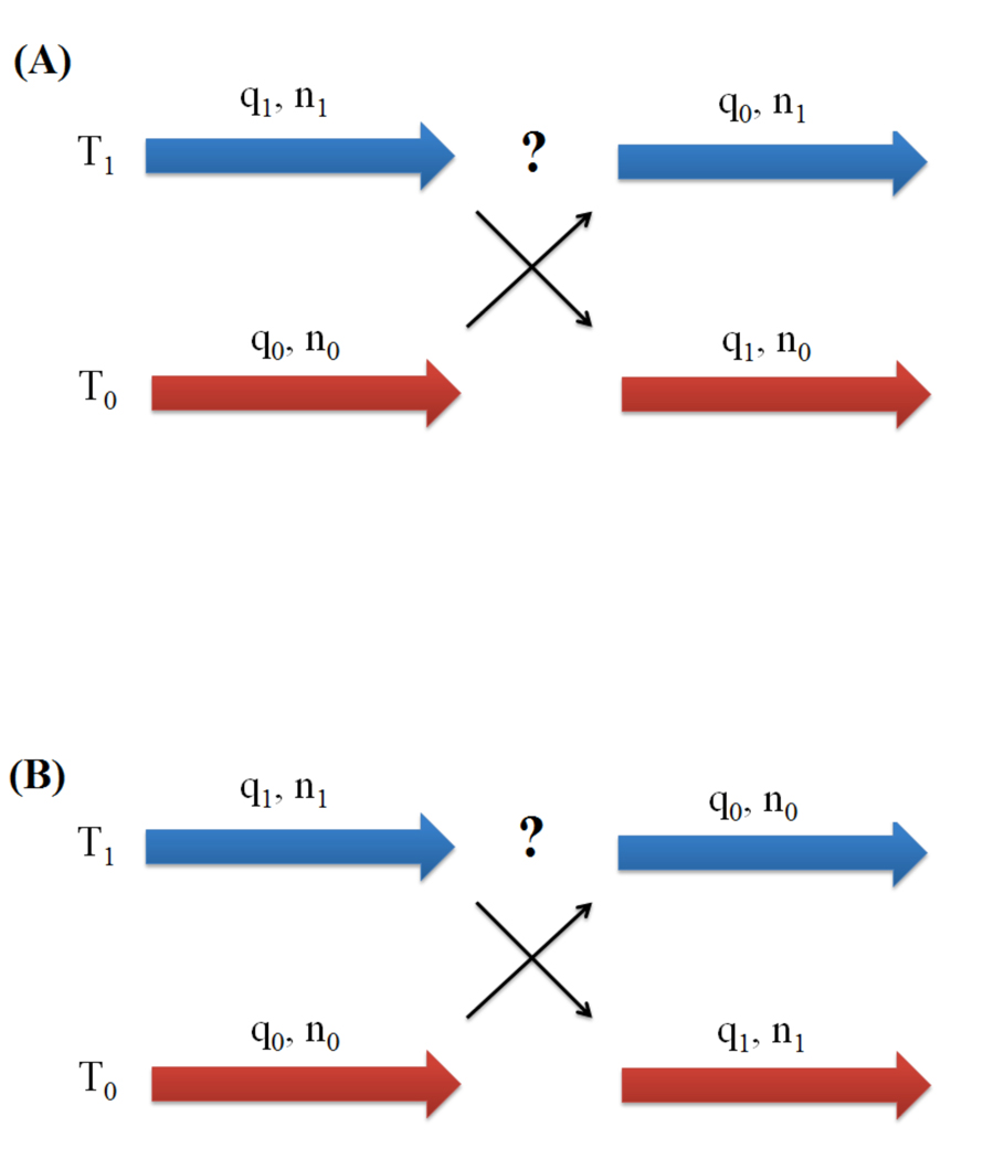
In the case of constant pH molecular dynamics, the potential energy of the system depends not only on the protein structure but also on the protein protonation state. Likewise, when coupling REMD algorithm with constant-pH MD, one can either attempt to exchange molecular structures only or swap both structures and protonation states at the same time. For simplicity, let us consider two replicas where replica 0 has temperature T0, protein structure q0 and protonation state n0, while replica 1 has temperature T1, structure q1 and protonation state n1. A diagrammatic description of the two exchange algorithms is shown in Figure 1. The first way of performing an exchange attempt is that replica 0 tries to jump from state (q0, n0) to state (q1, n0) at temperature T0 in one Monte Carlo step. Similarly, replica 1 attempts to transit from state (q1, n1) to state (q0, n1) at temperature T1. Protonation states are kept at exchange attempts and only change during dynamics. Therefore, the detailed balance equation now becomes:
| (11) |
Here w(β0q0n0, β1q1n1 → β0q1n0, β1q0n1);is the transition probability of swapping structures. If Metropolis criterion is used, this exchange probability can be written as:
| (12) |
and
| (13) |
where β0= 1/kBT0, β1= 1/kBT1 and E is the potential energy. Here, if the protonation states of two adjacent replicas at an exchange attempt are the same, the exchange probability of our constant pH REMD will be equivalent to the conventional REMD exchange probability. However, if it is not the case, four potential energy terms are needed to calculate exchange probability. Under this circumstance, the constant-pH REMD becomes a REMD algorithm that combines both temperature and Hamiltonian REMD algorithms.
Figure 1.
Diagrams displaying exchanging algorithms in constant-pH REMD. (A): Only molecular structures (denoted as q) are attempted to exchange. In this case, protonation states are not toughed at an exchange attempt; (B): Both molecular structures (denoted as q) and protonation states (denoted as n) are attempted to exchange at the same time. Metropolis criterion is applied in both algorithms to evaluate transitions.
One possible concern of exchanging only structures would be the role of kinetic energy, especially when n0 and n1 are different. In the REMD algorithm developed by Sugita and Okamoto, the kinetic energy terms in the Boltzmann factors cancel each other on average through velocity rescaling (Eq. 10). Only potential energies are required to compute exchange probabilities. There is a problem in canceling kinetic energy terms when the numbers of particles of two systems attempting to exchange are not the same. However, according to the constant-pH MD algorithm proposed by Mongan et al.62, a proton does not leave the molecule but becomes a dummy atom when an ionizable side chain is in a deprotonated state. Furthermore, that dummy atom retains its position and velocity which are controlled by molecular dynamics. Hence, the kinetic energy contributions to the Boltzmann weight will be cancelled out during exchange probability calculation, leaving only potential energy useful for the calculation.
The second possibility consists of exchanging protonation states as well as molecular structures at REMD Monte Carlo moves. For instance, replica 0 attempts to move from state (q0, n0) to state (q1, n1) at temperatures T0 in one MC move and replica 1 attempts to jump from state (q1, n1) to state (q0, n0) at temperature T1. The detailed balance equation now can be written as:
| (14) |
This equation states that the exchange probability is the product of MC transition probabilities at temperature T0 and T1. If the protonation states of two adjacent replicas are the same at an exchange attempt, the exchange probability of constant-pH REMD becomes the exchange probability of conventional temperature-based REMD. If n0 and n1 are different, then each MC transition is essentially the protonation state change step in constant-pH MD, plus a structural transition. For example, consider the MC transition at temperature T0,
| (15) |
where
| (16) |
The first term in Δ1 derives from the transition in configuration at fixed protonation state n0, and the rest corresponds to protonation state change at fixed structure q1. Eelec represents the electrostatic component of potential energy. Similarly, the transition probability of MC jump at T1 can be expressed as:
| (17) |
where
| (18) |
Therefore, according to Eq. 14, the exchange probability can be written as:
| (19) |
and
| (20) |
where Δ is the same quantity as in Eq. 13.
The exchange probability calculation in the second method of coupling REMD and constant-pH MD utilizes the same number of energy evaluations required by the first method since obtaining electrostatic potential energies does not require extra energy calculations. The advantage of implementing the second exchanging protocol (exchange both structures and protonation states) over the first one (exchange structures only) should not be significant because it is the conformational sampling at higher temperature that greatly improves conformational sampling at lower temperatures. Allowing protonation states to change at exchange attempts does not provide extra gains in conformational sampling since the protonation state space is well sampled during the MD propagation. Therefore, only the first method of performing exchanges was implemented.
D. Simulation Details
For our study, constant pH REMD simulations were carried out first on five reference compounds: blocked Aspartate, Glutamate, Histidine-δ, Lysine and Tyrosine to test our method and implementation. The experimental pKa values of those reference compounds are known80 and listed in Table 1. We later performed constant pH REMD simulations on a model peptide ADFDA (Ala-Asp-Phe-Asp-Ala, unblocked termini) and a heptapeptide derived from OMTKY3 (residues 26 to 32 with blocked termini). Four replicas were used in the reference compounds and ADFDA REMD simulations. The temperatures were 240, 300, 370 and 460 K for all six molecules. The pH range for the study of acidic side chains was sampled from 2.5 to 6 and the pH range of histidine is from 5.5 to 8. The basic side chains were titrated from pH 9 to 12. An interval of 0.5 was chosen for all titrations.
Table 1.
The REMD pKa predictions of reference compounds
| pKa | Aspartate | Glutamate | Histidine | Lysine | Tyrosine |
|---|---|---|---|---|---|
| REMD | 3.97(0.01) | 4.41(0.01) | 6.40(0.03) | 10.42(0.01) | 9.61(0.01) |
| Reference | 4.0 | 4.4 | 6.5 | 10.4 | 9.6 |
The numbers in parenthesis are the standard errors.
Eight replicas were chosen for the heptapeptide with a temperature range from 250 to 480 K. 10 ns were used for each replica in all REMD simulations and an exchange was attempted every 2 ps. A MC move to change protonation state was attempted every 10 fs. A second set of REMD runs was done with the same overall conditions but different initial structures in order to check simulation convergence.
To compare conformational and protonation state sampling, 100 ns of constant pH MD simulations were carried out for the aspartate reference compound and ADFDA, at the same pH values as in the REMD runs. For the heptapeptide, one set of 10 ns constant pH MD simulations were done at each pH values simulated by REMD method.
Constant pH REMD and MD simulations were done using the AMBER 10 molecular simulation suite.81 The AMBER ff99SB force field82 was used in all the simulations. The SHAKE algorithm83 was used to constrain the bonds connecting hydrogen atoms in all the simulations which allowed use of a 2 fs time step. OBC Generalized Born implicit solvent model66 was used to model water environment in all our calculations. The Berendsen thermostat84, with a relaxation time of 2 ps, was used to keep the replica temperature around their target values. Salt concentration (Debye-Huckel based) was set at 0.1M. The cutoff for non-bonded interaction and the Born radii was 30 Å.
E. Cluster Analysis
Cluster analysis was done using the Moil-View program85 in order to compare conformational sampling86,87. The MD and REMD trajectories (having same number of frames) at 300K and under the same solvent pH were combined following a procedure introduced in the paper of Okur et al.. Then the combined trajectory was clustered based on peptide backbone atoms root-mean-square deviations (RMSD). The population fraction corresponding to each cluster was obtained for MD and REMD simulation. The correlation coefficient values which represent the correlations between MD and REMD cluster population were calculated at each solution pH value by doing linear regression. A high correlation between MD and REMD cluster population indicates that the structure ensembles are close to each other. This method provides a direct comparison of global conformational sampling between MD and REMD simulations. The same technique was used when studying convergence of constant pH REMD and MD trajectories. A cluster cutoff RMSD of 1.5 Å is chosen for both ADFDA and the heptapeptide during our analysis.
F. Local Conformational Sampling and Its Convergence to the Final State
In our study, the local conformational sampling was examined by comparing the probability density of backbone dihedral angle pair (φ, ψ). Essentially, we are comparing the Ramachandran plot of a residue. Each (φ, ψ) probability density was computed by binning φ and ψ angle pairs 10° × 10°. These two dimensional histograms were normalized into populations and the contours were plotted. The metric used to evaluate (φ, ψ) probability density convergence was the root-mean-squared deviation (RMSD) between the cumulative (φ, ψ) histogram and the one produced by using all configurations. Each cumulative histogram was constructed by using (φ, ψ) pairs up to current time and following the same algorithm mentioned earlier in this section.
Results and Discussion
A. Reference Compounds
We first applied our constant pH REMD method to the reference compounds. Table 1 shows the pKa values predicted by REMD simulations (10 ns for each replica) as well as the reference pKa values. All our pKa values were calculated by fitting to the HH equation. Agreement between constant pH REMD predictions and the reference values can be seen.
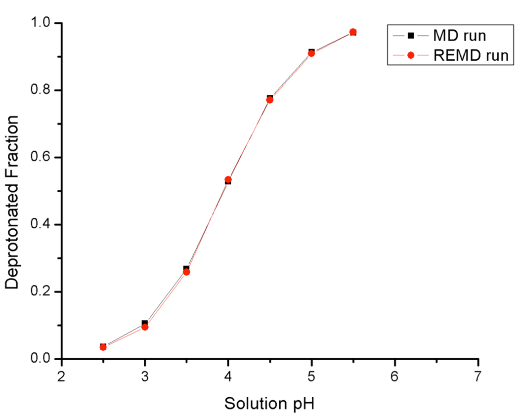
The pH titration curves of the same reference compounds showed agreement between MD (100 ns) and REMD simulations. Figure 2 demonstrates the REMD and MD titration curves of aspartic acid reference compound as an example.
Figure 2.
Titration curves of blocked aspartate amino acid from 100 ns MD at 300K and REMD runs. Agreement can be seen between MD and REMD simulations.
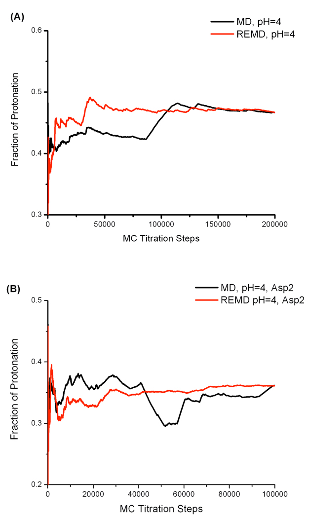
We further studied the convergence of protonation states sampling. REMD and MD protonation fraction were plotted with respect to MC attempts for aspartate reference compound at all pH values. Figure 3A demonstrates the protonated fraction versus time at pH 4 as one example. According to Figure 3A, it suggests that although the final pKa predictions are the same for REMD and MD simulations, the protonation state sampling during REMD simulations clearly converges faster than that in a MD run.
Figure 3.
Cumulative average protonation fraction of a titratable residue vs Monte Carlo (MC) steps. (A) Aspartic acid reference compound at pH=4. (B) Asp2 in model peptide ADFDA at pH=4.
B. Model peptide ADFDA
The model peptide ADFDA (as zwitterion) was chosen as a more stringent test of our constant pH REMD method. The charged termini will provide different electrostatic environment for each titratable Asp residue and hence a correct constant pH REMD model should reflect this difference between titration curves of the two Asp residues. The Asp2 residue is closer to the NH3+, so the deprotonated state is favored and the pKa value of Asp2 residue should shift below 4.0 (which is the pKa of the reference aspartic dipeptide). The Asp4 residue is closer to the COO− negative charge and hence the pKa value should shift above 4.0.
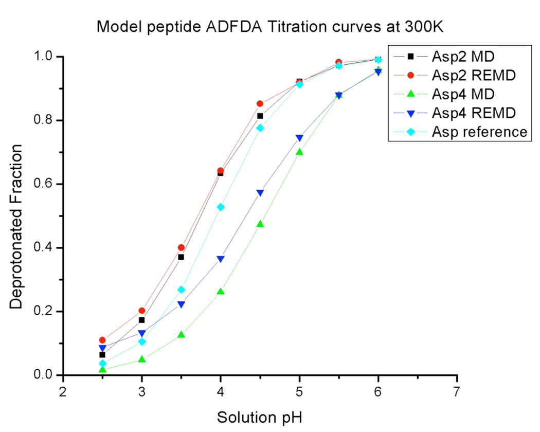
The titration curves of the model peptide ADFDA from REMD simulations are shown in Figure 4. We can clearly see that Asp2 and Asp4 have different titration curves from each other and from the reference compound. The pKa value and Hill coefficient for each Asp residue were obtained by fitting titration curves to a Hill plot. The results are shown in Table 2. The REMD pKa predictions reflect the difference between Asp2 and Asp4 due to different peptide electrostatic environments. We also displayed the MD titration curves of Asp2 and Asp4 in Figure 4 and listed the MD pKa predictions and corresponding Hill coefficients in Table 2. The titration curve of Asp2 residue only showed a small difference between MD and REMD simulation. But we can see differences in titration behaviors of Asp4 between MD and REMD calculations when solution pH is below 5. Interestingly, Lee et al. studied blocked Asp-Asp peptide using CPHMD method55, reporting different Hill coefficient for each of the two Asp residues.
Figure 4.
The titration curves of the model peptide ADFDA at 300K from both MD and REMD simulations. MD simulation time was 100 ns and 10 ns were chosen for each replica for REMD runs.
Table 2.
pKa predictions and Hill coefficients fitted from the HH equation
| Asp2 | Asp4 | |||
|---|---|---|---|---|
| pKa | Hill Coefficient | pKa | Hill Coefficient | |
| REMD | 3.74 | 0.87 | 4.38 | 0.67 |
| MD | 3.76 | 0.89 | 4.54 | 0.85 |
Convergence rates of Asp2 titration behavior were compared between REMD and MD calculations due to the fact that Asp2 titration curves are very close. The cumulative protonated fractions versus MC attempts at pH 4 are shown in Figure 3B. Faster convergence in protonation state sampling can be seen for REMD simulation even though both REMD and MD calculations resulted in the same final protonated fraction. Clearly, our constant pH REMD method accelerates the convergence of sampling of protonation states.
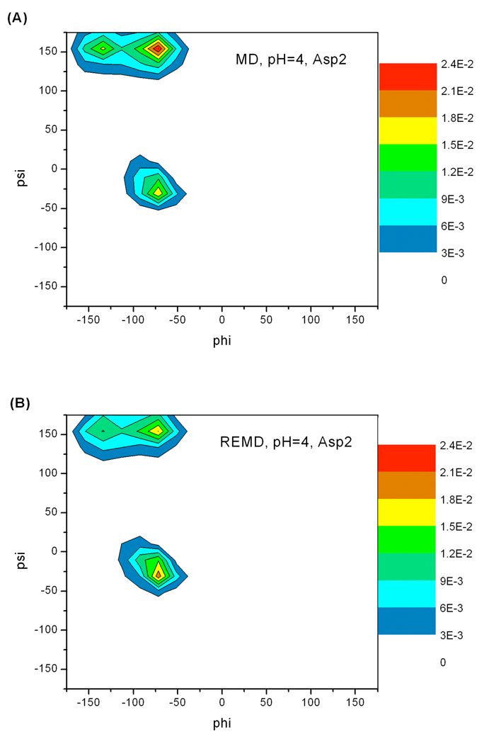
In addition to protonation state sampling, we also evaluated the conformational sampling in constant pH MD and REMD simulations. First, distribution of backbone φ and ψ angle pairs (Ramachandran plots) of residue Asp2, Phe3 and Asp4 in ADFDA at each solution pH were studied. The regions in Ramachandran plots sampled by MD and REMD simulations are the same. Ramachandran plots for residue Asp2 at pH 4 are shown in Figure 5 as an example.
Figure 5.
Backbone dihedral angle (φ, ψ) normalized probability density (Ramachandran plots) for Asp2 at pH 4 in ADFDA. Ramachandran plots at other solution pH values are similar. For Asp2, constant-pH MD and REMD sampled the same local backbone conformational space. Phe3 and Asp4 Ramachandran plots also display the same trend.
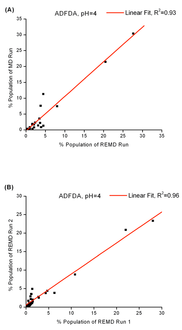
Since the Ramachandran plots only represent local conformational sampling, we also evaluated global conformational sampling by clustering MD and REMD trajectories and comparing the cluster populations. The MD and REMD cluster population R2 values are listed in Table 3. A plot of cluster populations from MD and REMD trajectories at solution pH of 4 is shown in Figure 6A as an example. The large R2 values indicate that the MD and REMD sampled the same conformational space and generated the same structure ensemble. The small size of ADFDA and simple structure of each residue make 100 ns long enough for MD to sample the relevant conformations.
Table 3.
Correlation coefficient between MD and REMD cluster populations
| pH=2.5 | pH=3 | pH=3.5 | pH=4 | |
|---|---|---|---|---|
| R2 | 0.94 | 0.90 | 0.79 | 0.93 |
| pH=4.5 | pH=5 | pH=5.5 | pH=6 | |
| R2 | 0.85 | 0.98 | 0.92 | 0.96 |
The R2 values were calculated by linear regression.
Figure 6.
Cluster populations of ADFDA at 300K (A): MD vs REMD at pH 4, (B): two REMD runs from different starting structures at pH 4. Large correlation shown in Figure 5B suggests that the REMD runs are converged. Large correlations between two independent REMD runs are also observed at other solution pH values. Correlations between MD and REMD simulations can be found in Table. 3.
We further studied the convergence of REMD simulations by comparing global conformation distribution between two REMD simulations starting from two different structures. Cluster populations of the two REMD simulations at solution pH 4 are displayed in Figure 6B. The R2 value is 0.959 at pH 4. This large correlation tells us that the two REMD simulations provide the same structure ensemble and hence the two simulations are converged.
C. Heptapeptide derived from OMTKY3
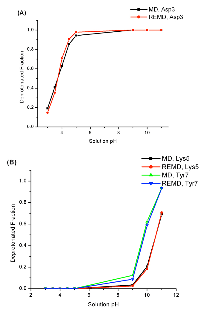
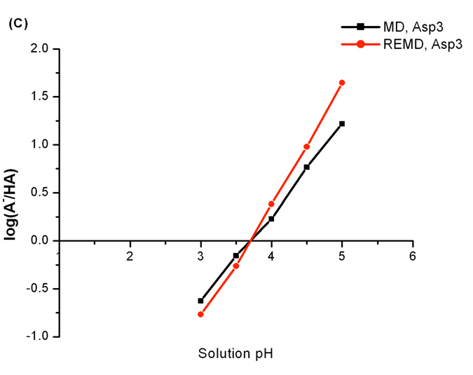
We first compared the protonation state sampling between constant pH REMD and MD simulations. Titration curves of Asp3, Lys5 and Tyr7 from two sets of simulations are plotted in Figure 7A and 7B. For each titratable residue, titration curves generated by constant pH REMD and MD are close to each other. Since the pKa value of Asp3 in this heptapeptide is experimentally determined to be 3.6, it will be interesting to evaluate how our predicted values compare to the experimental result. The pKa values of Asp3 were calculated based on Hill’s plots which are displayed in Figure 7C. The predicted pKa value is 3.7 for both REMD and MD simulations and they are in excellent agreement with the experimental pKa value. Following the same procedures, our predicted pKa values of Lys5 (10.6 for both REMD and MD) and Tyr7 (9.9 and 9.8 for REMD and MD respectively) were obtained. Not surprisingly, the REMD and MD schemes yielded essentially the same predicted pKa values for Lys5 and Tyr7.
Figure 7.
(A) and (B) are titration curves of Asp3, Lys5 and Tyr7 in the heptapeptide derived from protein OMTKY3. (C) shows the Hill’s plots of Asp3. The pKa values of Asp3 are found through Hill’s plots.
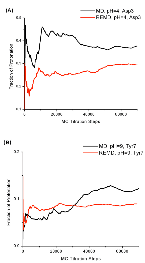
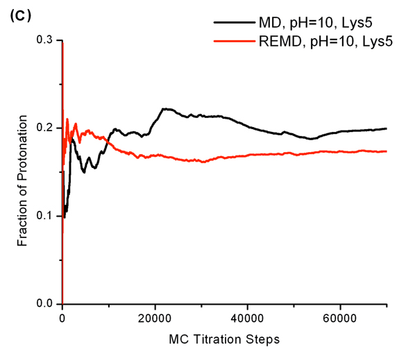
Although the final pKa predictions are the same for constant pH REMD and MD simulations, constant pH REMD showed clear advantage in the convergence of protonation state sampling. Again, we chose the cumulative average protonation fraction vs MC steps to reflect protonation state sampling convergence for all three titratable residues. Several representative plots are shown in Figure 8. The trend that constant pH REMD simulations produce faster convergence in protonation fraction is universal. Therefore, it is very clear that constant pH REMD method is better than constant pH MD in protonation state sampling.
Figure 8.
Cumulative average protonation fraction of a titratable residue vs MC steps.
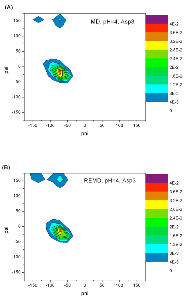
Conformational sampling is an important issue in constant pH studies. We first looked at the conformational sampling on peptide backbones. We evaluated backbone conformational sampling through Ramachandran plots. Six residues (from Ser2 to Tyr7) are studied here. Not surprisingly, Ramachandran plots from constant pH REMD and MD simulations are very close, suggesting that the overall local conformational samplings are similar. The Ramachandran plots of Asp3 at pH 4 are shown in Figure 9 as examples. The only exception is Tyr7 in acidic pH values. Tyr7 can visit the left-handed alpha helix conformation during constant pH REMD runs but is not able to do that in constant pH MD runs. In general, constant pH REMD and MD yielded the same Ramachandran plots for the heptapeptide.
Figure 9.
Dihedral angle (φ, ψ) probability densities of Asp3 at pH 4. (A): constant-pH MD results; (B): constant-pH REMD results. All others also show very similar trend.
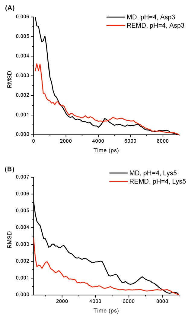
As demonstrated earlier, the overall samplings of (φ, ψ) distribution by constant pH REMD and MD are similar for Ser2 to Thr6. It is interesting to determine how fast each sampling scheme reaches the final distribution. We studied evolution of backbone conformational sampling based on cumulative data as what we did in the case of protonation state sampling convergence. As described in the METHOD section F, the RMSD between the (φ, ψ) probability distribution up to current time versus total simulation time was calculated. The smaller a RMSD is, the closer a probability distribution reaches to the final distribution. Deviations were calculated starting from the second nanosecond with time intervals incremented by 100 ps. The cumulative time-dependence RMSD of Asp3 and Lys5 are also shown in Figure 10 as examples. As seen in the figures, these curves decrease faster in constant pH REMD simulations. Figure 10 suggests that although the final (φ, ψ) probability distributions are similar between constant pH REMD and MD simulations, the constant pH REMD simulation clearly reaches the final state faster.
Figure 10.
The root-mean-square deviations (RMSD) between the cumulative (φ, ψ) probability density up to current time and the (φ, ψ) probability density produced by entire simulation. (φ, ψ) probability density convergence behaviors at other pH values also show that REMD runs converge to final distribution faster.
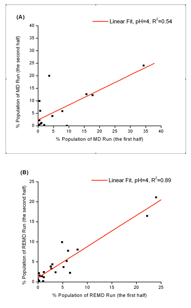
Cluster analysis was also applied to study the convergence of conformation sampling in the heptapeptide. By comparing cluster populations between the first and second half of one trajectory, one could check the convergence of that simulation. The two halves of a structural ensemble should yield the same populations in each cluster if convergence is reached. For example, simulations at pH 4, both constant pH REMD and MD yield about 20 clusters and the correlations coefficients are calculated through a linear regression. Cluster population plots and correlation coefficients are shown in Figure 11. A much higher correlation coefficient can be seen in constant pH REMD simulation, suggesting the two halves of the constant pH REMD simulation at pH 4 populate each cluster much more similarly than the corresponding constant pH MD does. Hence, much better convergence is achieved by the constant pH REMD run.
Figure 11.
Cluster population at 300 K from constant pH MD and REMD simulations at pH=4. Cluster analysis is performed using the entire simulation. The populations in each cluster from the first and second half of the trajectory are compared and plotted. Ideally, a converged trajectory should yield a correlation coefficient to be 1. (A): constant pH MD (B): constant pH REMD. Much higher correlation coefficient can be seen in constant pH REMD simulation, suggesting much better convergence is achieved by the constant pH REMD run.
Conclusion
In our work, we have applied replica exchange molecular dynamics (REMD) algorithm to the discrete protonation state model developed by Mongan et al.62 in order to study pH-dependent protein structure and dynamics. Seven small peptides were selected to test our constant pH REMD method. Constant pH molecular dynamics (MD) simulations were ran on the same peptides for comparison. The constant REMD method results are encouraging. The constant REMD method can predict pKa values in agreement with literature and experimental results. Constant pH REMD method also displays advantage in convergence behaviors during protonation states and conformational sampling.
The REMD algorithm has been proven beneficial to study pH-dependent protein structures. Our future work will include studies of pH-dependent protein dynamics and application of this constant pH REMD to large proteins.
Acknowledgment
We thank Carlos Simmerling and Wei Yang for helpful discussions. This work is supported from National Institute of Health under Contract 1R01 AI073674. Computer resources and support were provided by the Large Allocations Resource Committee through grant TG-MCA05S010 and the University of Florida High-Performance Computing Center.
References
- 1.Matthew JB, Gurd FRN, Garciamoreno EB, Flanagan MA, March KL, Shire SJ. Crc Cr. Rev. Bioch. Mol. 1985;18:91–197. doi: 10.3109/10409238509085133. [DOI] [PubMed] [Google Scholar]
- 2.Mongan J, Case DA. Curr. Opin. Struct. Biol. 2005;15:157–163. doi: 10.1016/j.sbi.2005.02.002. [DOI] [PubMed] [Google Scholar]
- 3.Yang AS, Honig B. J. Mol. Biol. 1993;231:459–474. doi: 10.1006/jmbi.1993.1294. [DOI] [PubMed] [Google Scholar]
- 4.Bierzynski A, Kim PS, Baldwin RL. Proc. Natl. Acad. Sci. U. S. A. 1982;79:2470–2474. doi: 10.1073/pnas.79.8.2470. [DOI] [PMC free article] [PubMed] [Google Scholar]
- 5.Shoemaker KR, Kim PS, Brems DN, Marqusee S, York EJ, Chaiken IM, Stewart JM, Baldwin RL. Proc. Natl. Acad. Sci. U. S. A. 1985;82:2349–2353. doi: 10.1073/pnas.82.8.2349. [DOI] [PMC free article] [PubMed] [Google Scholar]
- 6.Schaefer M, Van Vlijmen HWT, Karplus M. Adv. Protein Chem. 1998;51:1–57. doi: 10.1016/s0065-3233(08)60650-6. [DOI] [PubMed] [Google Scholar]
- 7.Antosiewicz J, Briggs JM, McCammon JA. Eur. Biophys. J. Biophy. 1996;24:137–141. doi: 10.1007/BF00180270. [DOI] [PubMed] [Google Scholar]
- 8.Hunenberger PH, Helms V, Narayana N, Taylor SS, McCammon JA. Biochemistry. 1999;38:2358–2366. doi: 10.1021/bi982064g. [DOI] [PubMed] [Google Scholar]
- 9.Demchuk E, Genick UK, Woo TT, Getzoff ED, Bashford D. Biochemistry. 2000;39:1100–1113. doi: 10.1021/bi991513p. [DOI] [PubMed] [Google Scholar]
- 10.Dillet V, Dyson HJ, Bashford D. Biochemistry. 1998;37:10298–10306. doi: 10.1021/bi980333x. [DOI] [PubMed] [Google Scholar]
- 11.Harris TK, Turner GJ. IUBMB Life. 2002;53:85–98. doi: 10.1080/15216540211468. [DOI] [PubMed] [Google Scholar]
- 12.Kelly JW. Curr. Opin. Struct. Biol. 1996;6:11–17. doi: 10.1016/s0959-440x(96)80089-3. [DOI] [PubMed] [Google Scholar]
- 13.Kelly JW. Structure. 1997;5:595–600. doi: 10.1016/s0969-2126(97)00215-3. [DOI] [PubMed] [Google Scholar]
- 14.Rastogi VK, Girvin ME. Nature. 1999;402:263–268. doi: 10.1038/46224. [DOI] [PubMed] [Google Scholar]
- 15.Hill TL. J. Am. Chem. Soc. 1956;78:3330–3336. [Google Scholar]
- 16.Simonson T, Carlsson J, Case DA. J. Am. Chem. Soc. 2004;126:4167–4180. doi: 10.1021/ja039788m. [DOI] [PubMed] [Google Scholar]
- 17.Tanford C, Kirkwood JG. J. Am. Chem. Soc. 1957;79:5333–5339. [Google Scholar]
- 18.Warshel A. Nature. 1987;330:15–16. doi: 10.1038/330015a0. [DOI] [PubMed] [Google Scholar]
- 19.Langsetmo K, Fuchs JA, Woodward C. Biochemistry. 1991;30:7603–7609. doi: 10.1021/bi00244a032. [DOI] [PubMed] [Google Scholar]
- 20.Eberini I, Baptista AM, Gianazza E, Fraternali F, Beringhelli T. Proteins: Struct., Funct., Bioinf. 2004;54:744–758. doi: 10.1002/prot.10643. [DOI] [PubMed] [Google Scholar]
- 21.Sham YY, Muegge I, Warshel A. Biophys. J. 1998;74:1744–1753. doi: 10.1016/S0006-3495(98)77885-3. [DOI] [PMC free article] [PubMed] [Google Scholar]
- 22.Simonson T, Archontis G, Karplus M. J. Phys. Chem. B. 1999;103:6142–6156. [Google Scholar]
- 23.Warshel A, Aqvist J. Annu. Rev. Biophys. Biomol. Struct. 1991;20:267–298. doi: 10.1146/annurev.bb.20.060191.001411. [DOI] [PubMed] [Google Scholar]
- 24.Antosiewicz J, Mccammon JA, Gilson MK. J. Mol. Biol. 1994;238:415–436. doi: 10.1006/jmbi.1994.1301. [DOI] [PubMed] [Google Scholar]
- 25.Antosiewicz J, McCammon JA, Gilson MK. Biochemistry. 1996;35:7819–7833. doi: 10.1021/bi9601565. [DOI] [PubMed] [Google Scholar]
- 26.Bashford D, Karplus M. Biochemistry. 1990;29:10219–10225. doi: 10.1021/bi00496a010. [DOI] [PubMed] [Google Scholar]
- 27.Demchuk E, Wade RC. J. Phys. Chem. 1996;100:17373–17387. [Google Scholar]
- 28.Kamerlin SCL, Haranczyk M, Warshel A. J. Phys. Chem. B. 2009;113:1253–1272. doi: 10.1021/jp8071712. [DOI] [PMC free article] [PubMed] [Google Scholar]
- 29.Riccardi D, Schaefer P, Cui Q. J. Phys. Chem. B. 2005;109:17715–17733. doi: 10.1021/jp0517192. [DOI] [PubMed] [Google Scholar]
- 30.Warshel A, Sussman F, Hwang JK. J. Mol. Biol. 1988;201:139–159. doi: 10.1016/0022-2836(88)90445-7. [DOI] [PubMed] [Google Scholar]
- 31.Bas DC, Rogers DM, Jensen JH. Proteins: Struct., Funct., Bioinf. 2008;73:765–783. doi: 10.1002/prot.22102. [DOI] [PubMed] [Google Scholar]
- 32.Li H, Robertson AD, Jensen JH. Proteins: Struct., Funct., Bioinf. 2005;61:704–721. doi: 10.1002/prot.20660. [DOI] [PubMed] [Google Scholar]
- 33.Alexov EG, Gunner MR. Biophys. J. 1997;72:2075–2093. doi: 10.1016/S0006-3495(97)78851-9. [DOI] [PMC free article] [PubMed] [Google Scholar]
- 34.Baptista AM. J. Chem. Phys. 2002;116:7766–7768. [Google Scholar]
- 35.Baptista AM, Martel PJ, Petersen SB. Proteins. 1997;27:523–544. [PubMed] [Google Scholar]
- 36.Baptista AM, Teixeira VH, Soares CM. J. Chem. Phys. 2002;117:4184–4200. [Google Scholar]
- 37.Georgescu RE, Alexov EG, Gunner MR. Biophys. J. 2002;83:1731–1748. doi: 10.1016/S0006-3495(02)73940-4. [DOI] [PMC free article] [PubMed] [Google Scholar]
- 38.Jensen JH, Li H, Robertson AD, Molina PA. J. Phys. Chem. A. 2005;109:6634–6643. doi: 10.1021/jp051922x. [DOI] [PubMed] [Google Scholar]
- 39.Khandogin J, Brooks CL. Biophys. J. 2005;89:141–157. doi: 10.1529/biophysj.105.061341. [DOI] [PMC free article] [PubMed] [Google Scholar]
- 40.Khandogin J, Brooks CL. Biochemistry. 2006;45:9363–9373. doi: 10.1021/bi060706r. [DOI] [PubMed] [Google Scholar]
- 41.Khandogin J, Brooks CL. Proc. Natl. Acad. Sci. U. S. A. 2007;104:16880–16885. doi: 10.1073/pnas.0703832104. [DOI] [PMC free article] [PubMed] [Google Scholar]
- 42.Khandogin J, Chen JH, Brooks CL. Proc. Natl. Acad. Sci. U. S. A. 2006;103:18546–18550. doi: 10.1073/pnas.0605216103. [DOI] [PMC free article] [PubMed] [Google Scholar]
- 43.Khandogin J, Raleigh DP, Brooks CL. J. Am. Chem. Soc. 2007;129:3056–3057. doi: 10.1021/ja0688880. [DOI] [PMC free article] [PubMed] [Google Scholar]
- 44.Lee AC, Yu JY, Crippen GM. J. Chem. Inf. Model. 2008;48:2042–2053. doi: 10.1021/ci8001815. [DOI] [PubMed] [Google Scholar]
- 45.Livesay DR, Jacobs DJ, Kanjanapangka J, Chea E, Cortez H, Garcia J, Kidd P, Marquez MP, Pande S, Yang D. J. Chem. Theory Comput. 2006;2:927–938. doi: 10.1021/ct600066z. [DOI] [PubMed] [Google Scholar]
- 46.Machuqueiro M, Baptista AM. J. Phys. Chem. B. 2006;110:2927–2933. doi: 10.1021/jp056456q. [DOI] [PubMed] [Google Scholar]
- 47.Machuqueiro M, Baptista AM. Biophys. J. 2007;92:1836–1845. doi: 10.1529/biophysj.106.092445. [DOI] [PMC free article] [PubMed] [Google Scholar]
- 48.Machuqueiro M, Baptista AM. Proteins: Struct., Funct., Bioinf. 2008;72:289–298. doi: 10.1002/prot.21923. [DOI] [PubMed] [Google Scholar]
- 49.Machuqueiro M, Baptista AM. J. Am. Chem. Soc. 2009;131:12586–12594. doi: 10.1021/ja808463e. [DOI] [PubMed] [Google Scholar]
- 50.Madura JD, Briggs JM, Wade RC, Davis ME, Luty BA, Ilin A, Antosiewicz J, Gilson MK, Bagheri B, Scott LR, Mccammon JA. Comput. Phys. Commun. 1995;91:57–95. [Google Scholar]
- 51.Minikis RM, Kairys V, Jensen JH. J. Phys. Chem. A. 2001;105:3829–3837. [Google Scholar]
- 52.Mertz JE, Pettitt BM. Int. J. Supercomput. Ap. 1994;8:47–53. [Google Scholar]
- 53.Borjesson U, Hunenberger PH. J. Chem. Phys. 2001;114:9706–9719. [Google Scholar]
- 54.Borjesson U, Hunenberger PH. J. Phys. Chem. B. 2004;108:13551–13559. [Google Scholar]
- 55.Lee MS, Salsbury FR, Brooks CL. Proteins: Struct., Funct., Bioinf. 2004;56:738–752. doi: 10.1002/prot.20128. [DOI] [PubMed] [Google Scholar]
- 56.Kong XJ, Brooks CL. J. Chem. Phys. 1996;105:2414–2423. [Google Scholar]
- 57.Burgi R, Kollman PA, van Gunsteren WF. Proteins. 2002;47:469–480. doi: 10.1002/prot.10046. [DOI] [PubMed] [Google Scholar]
- 58.Dlugosz M, Antosiewicz JM. Chem. Phys. 2004;302:161–170. [Google Scholar]
- 59.Dlugosz M, Antosiewicz JM. J. Phys. Chem. B. 2005;109:13777–13784. doi: 10.1021/jp0505779. [DOI] [PubMed] [Google Scholar]
- 60.Dlugosz M, Antosiewicz JM. J. Phys.: Condens. Matter. 2005;17:S1607–S1616. [Google Scholar]
- 61.Dlugosz M, Antosiewicz JM, Robertson AD. Phys. Rev. E. 2004;69:021915. doi: 10.1103/PhysRevE.69.021915. [DOI] [PubMed] [Google Scholar]
- 62.Mongan J, Case DA, McCammon JA. J. Comput. Chem. 2004;25:2038–2048. doi: 10.1002/jcc.20139. [DOI] [PubMed] [Google Scholar]
- 63.Walczak AM, Antosiewicz JM. Phys. Rev. E. 2002;66:051911. doi: 10.1103/PhysRevE.66.051911. [DOI] [PubMed] [Google Scholar]
- 64.Metropolis N, Rosenbluth AW, Rosenbluth MN, Teller AH, Teller E. J. Chem. Phys. 1953;21:1087–1092. [Google Scholar]
- 65.Bashford D, Case DA. Annu. Rev. Phys. Chem. 2000;51:129–152. doi: 10.1146/annurev.physchem.51.1.129. [DOI] [PubMed] [Google Scholar]
- 66.Onufriev A, Bashford D, Case DA. J. Phys. Chem. B. 2000;104:3712–3720. [Google Scholar]
- 67.Hamelberg D, Mongan J, McCammon JA. J. Chem. Phys. 2004;120:11919–11929. doi: 10.1063/1.1755656. [DOI] [PubMed] [Google Scholar]
- 68.Hamelberg D, Mongan J, McCammon JA. Protein Sci. 2004;13:76–76. [Google Scholar]
- 69.Williams SL, de Oliveira CAF, McCammon JA. J. Chem. Theory Comput. 2010;6:560–568. doi: 10.1021/ct9005294. [DOI] [PMC free article] [PubMed] [Google Scholar]
- 70.Li HZ, Fajer M, Yang W. J. Chem. Phys. 2007;126:024106. doi: 10.1063/1.2424700. [DOI] [PubMed] [Google Scholar]
- 71.Mitsutake A, Sugita Y, Okamoto Y. Biopolymers. 2001;60:96–123. doi: 10.1002/1097-0282(2001)60:2<96::AID-BIP1007>3.0.CO;2-F. [DOI] [PubMed] [Google Scholar]
- 72.Zheng LQ, Chen MG, Yang W. Proc. Natl. Acad. Sci. U. S. A. 2008;105:20227–20232. doi: 10.1073/pnas.0810631106. [DOI] [PMC free article] [PubMed] [Google Scholar]
- 73.Zheng LQ, Chen MG, Yang W. J. Chem. Phys. 2009;130:234105. doi: 10.1063/1.3153841. [DOI] [PubMed] [Google Scholar]
- 74.Berg BA, Neuhaus T. Phys. Lett. B. 1991;267:249–253. [Google Scholar]
- 75.Berg BA, Neuhaus T. Phys. Rev. Lett. 1992;68:9–12. doi: 10.1103/PhysRevLett.68.9. [DOI] [PubMed] [Google Scholar]
- 76.Lyubartsev AP, Martsinovski AA, Shevkunov SV, Vorontsovvelyaminov PN. J. Chem. Phys. 1992;96:1776–1783. [Google Scholar]
- 77.Sugita Y, Okamoto Y. Chem. Phys. Lett. 1999;314:141–151. [Google Scholar]
- 78.Hansmann UHE. Chem. Phys. Lett. 1997;281:140–150. [Google Scholar]
- 79.Case DA, Cheatham TE, Darden T, Gohlke H, Luo R, Merz KM, Onufriev A, Simmerling C, Wang B, Woods RJ. J. Comput. Chem. 2005;26:1668–1688. doi: 10.1002/jcc.20290. [DOI] [PMC free article] [PubMed] [Google Scholar]
- 80.Bashford D, Case DA, Dalvit C, Tennant L, Wright PE. Biochemistry. 1993;32:8045–8056. doi: 10.1021/bi00082a027. [DOI] [PubMed] [Google Scholar]
- 81.Case DA, Darden TA, Cheatham TEI, Simmerling CL, Wang J, Duke RE, Luo R, Crowley M, Walker RC, Zhang W, Merz KM, Wang B, Hayik S, Roitberg A, Seabra G, Kolossváry I, Wong KF, Paesani F, Vanicek J, Wu X, Brozell SR, Steinbrecher T, Gohlke H, Yang L, Tan C, Mongan J, Hornak V, Cui G, Mathews DH, Seetin MG, Sagui C, Babin V, Kollman PA. AMBER. Vol. 10. San Francisco: University of California; 2008. [Google Scholar]
- 82.Hornak V, Abel R, Okur A, Strockbine B, Roitberg A, Simmerling C. Proteins: Struct., Funct., Bioinf. 2006;65:712–725. doi: 10.1002/prot.21123. [DOI] [PMC free article] [PubMed] [Google Scholar]
- 83.Ryckaert JP, Ciccotti G, Berendsen HJC. J. Comput. Phys. 1977;23:327–341. [Google Scholar]
- 84.Berendsen HJC, Postma JPM, Vangunsteren WF, Dinola A, Haak JR. J. Chem. Phys. 1984;81:3684–3690. [Google Scholar]
- 85.Elber R, Roitberg A, Simmerling C, Goldstein R, Li HY, Verkhivker G, Keasar C, Zhang J, Ulitsky A. Comput. Phys. Commun. 1995;91:159–189. [Google Scholar]
- 86.Okur A, Roe DR, Cui GL, Hornak V, Simmerling C. J. Chem. Theory Comput. 2007;3:557–568. doi: 10.1021/ct600263e. [DOI] [PubMed] [Google Scholar]
- 87.Okur A, Wickstrom L, Layten M, Geney R, Song K, Hornak V, Simmerling C. J. Chem. Theory Comput. 2006;2:420–433. doi: 10.1021/ct050196z. [DOI] [PubMed] [Google Scholar]


