Marginal Structural Models for Sufficient Cause Interactions

Abstract

Sufficient cause interactions concern cases in which there is a particular causal mechanism for some outcome that requires the presence of 2 or more specific causes to operate. Empirical conditions have been derived to test for sufficient cause interactions. However, when regression outcome models are used to control for confounding variables in tests for sufficient cause interactions, the outcome models impose restrictions on the relation between the confounding variables and certain unidentified background causes within the sufficient cause framework; often, these assumptions are implausible. By using marginal structural models, rather than outcome regression models, to test for sufficient cause interactions, modeling assumptions are instead made on the relation between the causes of interest and the confounding variables; these assumptions will often be more plausible. The use of marginal structural models also allows for testing for sufficient cause interactions in the presence of time-dependent confounding. Such time-dependent confounding may arise in cases in which one factor of interest affects both the second factor of interest and the outcome. It is furthermore shown that marginal structural models can be used not only to test for sufficient cause interactions but also to give lower bounds on the prevalence of such sufficient cause interactions.

In this paper, we describe how marginal structural models can be used in drawing inferences concerning sufficient cause interactions. Sufficient cause interactions are a particular type of mechanistic interaction and concern cases in which a particular causal mechanism for some outcome requires the presence of 2 or more specific causes to operate. Rothman (1) described the joint presence of 2 causes in the same causal mechanism as “synergism” and used the term “sufficient cause” to refer to each mechanism for the outcome. VanderWeele and Robins (2) formalized the sufficient cause framework in terms of counterfactuals and used counterfactuals to define the notion of a “sufficient cause interaction,” the presence of which implied synergism as Rothman had conceived it. VanderWeele and Robins (2, 3) also derived empirical conditions to test for sufficient cause interactions. Testing for such sufficient cause interactions may be of interest in initial attempts to explore possible biologic pathways for a particular outcome, specifically for exploring whether there might be a pathway that requires the presence of 2 particular causes to operate. A series of papers (3–6) have described various approaches to testing for sufficient cause interactions, including the use of t-test-like test statistics (3), regression models (4), and doubly robust and multiply robust tests (5).

Although the sufficient cause framework has, as of yet, seen relatively little empirical application in epidemiology, this arguably may be because of a lack of relevant empirical results and lack of adequate statistical methods to handle the framework. As described below, empirical results of interest are now available for the sufficient cause framework (2–4); in this paper, we hope to advance the statistical methods available to make use of these empirical results.

Specifically, the motivation for the present paper on marginal structural models (7, 8) for sufficient cause interactions is 2-fold. First, as described in greater detail below, within the sufficient cause framework, a regression model for the outcome that controls for confounding variables will impose certain restrictions on the relation between the confounding variables in the model and certain unidentified background causes within the sufficient cause framework. Often, these restrictions will be implausible. By using marginal structural models, rather than standard regression models, assumptions are instead made concerning the relations between the causes of interest and the confounding variables, and these assumptions will often be more plausible. Second, in some cases, the 2 causes may be such that one cause of interest affects the second cause. When variables are a consequence of the first cause of interest and also confound the relation between the second factor of interest and the outcome, then traditional regression methods cannot be used to estimate causal effects or to test for sufficient cause interactions. Marginal structural models can in fact be used to address issues of time-dependent confounding in testing for sufficient cause interactions in settings in which regression methods fail.

The remainder of the paper is structured as follows. First, we describe the sufficient cause framework and the empirical and counterfactual conditions for testing for sufficient cause interactions. We then describe how marginal structural models can be used for inference concerning sufficient cause interactions, including inference in settings in which time-dependent confounding may be present. We also discuss how marginal structural models circumvent a number of misspecification concerns about using regression models to test for sufficient cause interactions. It is furthermore noted that although a sufficient cause interaction potentially depends on the presence of a single individual exhibiting such an interaction, marginal structural models can be used to provide lower bounds on the prevalence of sufficient cause interactions in a population, that is, on the proportion of individuals for whom the outcome would occur if both X₁ and X₂ were present but would not occur if only one of the 2 exposures were present. The approach of using marginal structural models for inference concerning sufficient cause interactions is illustrated by examining interactions between the effects of exposure to arsenic from drinking water and to tobacco smoking on the development of premalignant skin lesions. We close with some further discussion.

THE SUFFICIENT CAUSE FRAMEWORK AND SUFFICIENT CAUSE INTERACTIONS

In this section, we give an overview of the sufficient cause framework and its relation to counterfactuals. We let D denote a binary outcome of interest and let X₁, X₂, …, X_n denote binary causes of interest that are potentially modifiable. For much of the discussion in this paper, we assume that there are only 2 causes of interest; the ideas, however, easily extend to 3 or more causes of interest. For some cause, X_i, we let $\stackrel{-}{X_i}$ denote the complement of X_i, that is, that the cause X_i is absent. We let D_x1x2(ω) denote the counterfactual value of D for individual ω if, possibly contrary to fact, there had been interventions to set X₁ = x₁ and to set X₂ = x₂. For each individual ω, there would thus be 4 possible counterfactual or potential outcomes D₁₁(ω), D₁₀(ω), D₀₁(ω), and D₀₀(ω) corresponding to what would have happened to that individual under the various possible exposure combinations. To make the discussion concrete, we consider an example in which our outcome, D, denotes skin lesions and our 2 exposures, X₁ and X₂, denote, respectively, high levels of well water arsenic exposure (>100 μg/L) and current or past tobacco smoking. We return to this example below.

When a particular outcome is in view, Rothman (1) conceived of the relation between cause and effect as a collection of causal mechanisms for D. Each causal mechanism would itself be sufficient for the outcome; thus, Rothman referred to these causal mechanisms as “sufficient causes.” Each mechanism might require some combination of the causes, X₁, X₂, …, X_n, either their presence or absence, to operate. Each causal mechanism might also require some additional background factors, other than X₁, X₂, …, X_n, to operate. For the kth mechanism, we denote the presence of these additional background factors as A_k = 1 and their absence as A_k = 0. The factors of interest in a particular study are denoted by the X_i variables; all other factors are considered background and are denoted by the A_k variables. Within Rothman's description, each mechanism or “sufficient cause” would consist of a minimal set of conditions or “component causes” such that, when all the component causes for a particular mechanism were present, the mechanism would operate and the outcome would inevitably occur. Within every sufficient cause, every component of that sufficient cause would be necessary for the corresponding mechanism to operate. Synergism would be said to be present between X_i and X_j if there were a sufficient cause that required both X_i and X_j to operate.

Consider the case of 2 causes of interest where, as above, X₁ denotes high levels of arsenic exposure and X₂ denotes smoking. We might be interested in whether there is a sufficient cause for the outcome D, skin lesions, which requires both X₁ and X₂ to operate. This would give us some understanding of the biologic pathways leading to the outcome. In the general case of 2 binary exposures, each sufficient cause for the outcome might require the presence of X₁, or the absence of X₁, or may not require either; similarly, each sufficient cause for the outcome D might require the presence of X₂, or the absence of X₂, or may not require either. Within the sufficient cause framework, we could thus enumerate 9 different sufficient causes for D: $A_0,A_1{X}_1,A_2{\stackrel{-}{X}}_1,A_3{X}_2,A_4{\stackrel{-}{X}}_2,A_5{X}_1{X}_2,A_6{\stackrel{-}{X}}_1{X}_2,$$A_7{X}_1{\stackrel{-}{X}}_2,$ and $A_8{\stackrel{-}{X}}_1{\stackrel{-}{X}}_2$ (2, 3, 9, 10). Here, the variables A_k denote factors other than the presence or absence of high levels of arsenic exposure, X₁, and smoking, X₂, that may be required for a particular mechanism to operate. These may be complex combinations of various other environmental and genetic factors that are unknown to the investigator. In this setting, if the sufficient cause A₅X₁X₂ is present, that is, if A₅ is not uniformly zero, then synergism is present between X₁ and X₂.

VanderWeele and Robins (2, 3) derived empirical conditions for testing for synergism. These conditions required control for confounding. We let C denote some set of variables for which data are available. We say that the effects of X₁ and X₂ on D are unconfounded given a set of variables C if P(D_x1x2|C = c) = P(D = 1|X₁ = x₁,X₂ = x₂,C = c), that is, if, within strata of C, individuals with a particular exposure combination X₁ = x₁, X₂ = x₂ are representative of what would have happened to everyone in that stratum if we had intervened to fix X₁ = x₁ and X₂ = x₂. The set C will generally need to contain all variables that affect both the outcome D and the exposures X₁ or X₂. The set of confounding variables C, however, will not in general need to contain everything that might be present in the background factors A_k; some factors captured by A_k (e.g., genetic factors) might cause the outcome D (e.g., skin lesions) but may be unrelated to the exposures X₁ and X₂ (e.g., arsenic and smoking) and thus would not be necessary to control for to avoid confounding.

VanderWeele and Robins (2, 3) showed that if the effects of X₁ and X₂ on D are unconfounded given a set of variables C, and if we let p_x1x2c = P(D = 1|X₁ = x₁, X₂ = x₂,C = c), then, if for some c,

(1)

then synergism between X₁ and X₂ must be present. Condition 1 is sufficient but not necessary for synergism.

VanderWeele and Robins (2) also related sufficient causes to counterfactuals and, in particular, showed that synergism must be present if there is an individual for whom

(2)

Condition 2 is equivalent to an individual for whom D₁₁(ω) = 1 and D₁₀(ω) = D₀₁(ω) = 0. Condition 2 is more general than condition 1 in that if 1 is satisfied then 2 must be satisfied for some individual ω, but 2 may be satisfied for some individual ω without 1 being satisfied. Essentially, condition 1 implies condition 2 and condition 2 implies the presence of synergism between X₁ and X₂. However, condition 1, unlike condition 2, can be tested by using data. VanderWeele and Robins (2) said that a sufficient cause interaction was present whenever condition 2 was satisfied. Condition 2 implies that there is some individual who would have the outcome if both X₁ and X₂ were present but who would not have the outcome if only one of X₁ or X₂ were present. Further details on the relations between counterfactuals and sufficient causes are available elsewhere (2, 3, 11).

In some cases, the effects of the cause X_i may be in the same direction for all individuals. For example, it may not be the case that X_i is causative for some individuals and preventive for others. We say that X₁ and X₂ have positive monotonic effects on D if D_x1x2(ω) is nondecreasing in x₁ and x₂ for all individuals ω (3, 12). For example, it seems unlikely that either high levels of arsenic exposure, X₁, or smoking, X₂, would prevent skin lesions for any individual, and we would thus say that these exposures have monotonic effects on the outcome. When X₁ and X₂ have positive monotonic effects on D, then a condition weaker than 1 can be used to test for sufficient cause interactions. In particular, if the effects of X₁ and X₂ on D are unconfounded given C, then a sufficient cause interaction must be present if, for some c, the following condition holds (2, 3, 13):

(3)

It can furthermore be shown (2) that, under the monotonicity assumption, a sufficient cause interaction is present if there is an individual ω for whom

(4)

Empirical and counterfactual conditions are also available for testing for 3-way or n-way interactions between binary exposures (2, 11).

MARGINAL STRUCTURAL MODELS FOR SUFFICIENT CAUSE INTERACTIONS

In this section and the one that follows, we focus on the use of marginal structural models (7, 8) in inference for sufficient cause interactions. A marginal structural model is a model for expected counterfactual outcomes, that is, a model for 𝔼[D_x1x2], whereas ordinary regression models are models for expected outcomes conditional on covariates. Thus, a regression model might be a model for the conditional expected outcome 𝔼[D|X₁ = x₁, X₂ = x₂, C = c]. For example, a Bernoulli regression model for 𝔼[D|X₁ = x₁, X₂ = x₂, C = c] with identity link might take the form

(5)

If C is multivariate, then α₄ will be a vector. If the effects of X₁ and X₂ on D are unconfounded given C, then 𝔼[D|X₁ = x₁,X₂ = x₂,C = c] = 𝔼[D_x1x2|C = c] and model 5 can be used to estimate causal effects within strata of C provided that model 5 is correctly specified. Often, when the outcome is binary, log-linear or logistic regression is used rather than linear regression. A model such as 5 is a model for the expected observed outcome conditional on the covariates. In contrast, a marginal structural model for the effects of X₁ and X₂ on D is a model for counterfactuals and might take the form

(6)

If the effects of X₁ and X₂ on D are unconfounded without conditioning on covariates, that is, C = Ø (e.g., if X₁ and X₂ are randomized), then the model coefficients (α₀, α₁, α₂, α₃) and (β₀, β₁, β₂, β₃) coincide. If conditioning on C does not suffice to control for confounding, then the regression coefficients (α₀, α₁, α₂, α₃) will not in general admit a causal interpretation.

The parameters of a marginal structural model are typically fit by using inverse probability of treatment weighting (7) under assumptions of no unmeasured confounding, given below. This estimation method by weighting has the advantage that it can be used in the presence of time-dependent confounding. Time-dependent confounding is said to be present when a variable, say L, is the effect of some exposure, say X₁, but also affects both a subsequent exposure, X₂, and the outcome, D, and we wish to assess the joint effects of X₁ and X₂ on D. Further discussion of time-dependent confounding as it relates to inference concerning sufficient cause interactions is given in Appendix 1. The main point to be emphasized here is that inverse probability weighting can be used to fit a marginal structural model even in the presence of such time-dependent confounding, whereas estimators of the parameters of the outcome regression model in expression 5 will not give unbiased estimators of causal effects in the presence of time-dependent confounding.

Details for fitting marginal structural models are given elsewhere (7); here, we provide a brief overview of how the parameters of a model such as 6 can be estimated and how the marginal structural model can subsequently be used to test for the presence of sufficient cause interactions. As noted above, we let C denote some set of baseline confounding variables. We let L denote some set of variables that may be effects of exposure X₁ but may affect exposure X₂. In some cases, the set L may be empty; for instance, in the arsenic and smoking example, it seems unlikely that the effects of drinking from a well containing arsenic causes one to smoke, or vice versa. Following Robins et al. (7), if the effect of X₁ on D is unconfounded given C and the effect of X₂ on D is unconfounded given {C, L, X₁}, then we can estimate model 6 using inverse probability of treatment weighting by calculating the following weights:

and

where x_1ω, x_2ω, c_ω, and l_ω denote individual ω’s values of X₁, X₂, C, and L, respectively. The probabilities in the weights can be estimated by using regular logistic regression. Including the probability in the numerator is optional but can lead to more efficient estimators (7). To fit marginal structural model 6, one can use a weighted regression of D on X₁, X₂ and X₁ × X₂, where the weights are given by v_ω¹×v_ω². The estimators of the parameters from the weighted regression will yield consistent estimators of the parameters in marginal structural model 6. For the estimators of the standard errors to be valid, robust estimation of standard errors must be used (which generally give conservative estimates). Two technical assumptions should also be noted for these results to hold. First, causal inference in general requires a consistency assumption (14–17) that D_X1(ω)X2(ω) = D(ω), that is, that the outcome actually observed is equal to the outcome that would have been observed under interventions to set X₁ and X₂ to the levels that they actually were. Second, marginal structural models specifically require a positivity assumption (7, 8, 18) that 0 < P(X₁ = 1|C = c) < 1 for all c and 0 < P(X₂ = 1|X₁ = x₁, C = c, L = l) < 1 for all x₁, c, l, that is, that the probability of each exposure being present or absent is nonzero within each stratum defined by confounding variables. Refer to Robins et al. (7) for further details on fitting marginal structural models.

Marginal structural model 6 can be used in a relatively straightforward way to test for sufficient cause interaction. As above, there is a sufficient cause interaction if there is an individual for whom D₁₁(ω) – D₁₀(ω) – D₀₁(ω) > 0. Thus, if 𝔼[D₁₁ – D₁₀ – D₀₁] > 0, then there must be an individual for whom D₁₁(ω) – D₁₀(ω) – D₀₁(ω) > 0 and synergism is present between X₁ and X₂. From model 6, we have that

Thus, a test for β₃ – β₀ > 0 in marginal structural model 6 would constitute a test for a sufficient cause interaction between X₁ and X₂. Many software packages allow for tests of contrasts of regression coefficients such as β₃ – β₀ > 0.

We also noted above that if the effects of X₁ and X₂ on D were monotonic, then a sufficient cause interaction is present if D₁₁(ω) – D₁₀(ω) – D₀₁(ω) + D₀₀(ω) > 0. Thus, if we have on average that 𝔼[D₁₁ – D₁₀ – D₀₁ + D₀₀] > 0, then a sufficient cause interaction must be present. The condition 𝔼[D₁₁ – D₁₀ – D₀₁ + D₀₀] > 0 can be reexpressed in terms of the coefficient in model 6 as β₃ > 0; so, under the monotonicity assumption, a test for β₃ > 0 in marginal structural model 6 would constitute a test for a sufficient cause interaction between X₁ and X₂. The approach of using marginal structural models can be used more generally to test for 3-way or n-way sufficient cause interactions. In these cases, a marginal structural model for 𝔼[D_x1x2x3] or 𝔼[D_x1…xn] can be fit by using inverse probability of treatment weighting and the model coefficients can be used to test the conditions on counterfactuals for sufficient cause interactions given in VanderWeele and Robins (2) and in VanderWeele (11).

In recent work, counterfactual conditions are given for sufficient cause interactions for categorical and ordinal exposures (19). The approach described here of using marginal structural models to test for sufficient cause interactions could be used for categorical and ordinal exposures as well, but multinomial or ordinal logistic regression, rather than ordinary logistic regression, would have to be used to estimate the treatment weights (7). Finally, for exposures that are continuous, we could consider defining a causal interaction to be present comparing exposure levels (x₁, x₂) with (x₁^′, x₂^′) if there is an individual ω such that D_x1x2(ω) = 1 but D_x^′1x2(ω) = D_x1x^′2(ω) = 0. The approach of using marginal structural models to test for causal interactions could potentially be used in this setting as well, but careful thought would have to be given to specifying the marginal structural model for 𝔼[D_x1x2]; furthermore, with continuous exposures, the weights involve densities rather than probabilities (7), and estimates are often less stable.

We noted above that marginal structural models can be used to test for sufficient cause interactions in settings with time-dependent confounding. However, this approach of using marginal structural models to test for sufficient cause interactions will likely be desirable even in settings in which time-dependent confounding is not present. Suppose that time-dependent confounding is not present and that the effects of X₁ and X₂ on D are unconfounded given some baseline covariates C. VanderWeele (4) discussed using linear models such as model 5 or log-linear models such as

(7)

or logistic models, to test for sufficient cause interactions. Such an approach requires that the outcome model be correctly specified.

The regression approach to testing for sufficient cause interactions can be problematic for several reasons. First, it may be difficult to correctly specify the main effect of C in models such as 5 or 7, and inference about model coefficients (α₀, α₁, α₂, α₃) will be valid only if the main effect of C is correctly specified, even though this main effect is not of primary interest. Second, for linear and log-linear models with continuous covariates C, the models may not give expected outcomes between 0 and 1. Third, in many settings, a model such as 7 may be misspecified because we might expect the effects of X₁ and X₂ to vary with C or we might expect the coefficients α₀, α₁, α₂, for instance, to depend on C (5). Fourth, VanderWeele (4) noted that within the sufficient cause framework, an outcome model such as 5 or 7 will impose certain restrictions on the relation between the confounding variables C and the background causes A₀, …, A₈. For example, in many cases, a model such as 5 will essentially require that the probabilities for the background factors A₁, …, A₈ of the sufficient causes involving X₁ and X₂ not depend on the covariates C; model 5 would essentially only allow the probability of the background factor A₀ for sufficient causes not involving X₁ and X₂ to depend on C. Such restrictions will often not be reasonable; refer to the Web Appendix for further discussion (this supplementary material is posted on the Journal's website (http://aje.oupjournals.org/)). The approach described above, however, of using marginal structural models to test for sufficient cause interactions circumvents many of these difficulties. In the marginal structural model approach, model 6 is saturated; thus, misspecification of the model is not an issue. However, the approach does require specifying a model for the probability of the exposures X₁ and X₂ conditional on the confounding variables C. In using the marginal structural model approach, no assumptions are imposed on the relation between C and the outcome Y or between C and the background causes A₀, …, A₈. The marginal structural model approach will give valid tests for sufficient cause interactions provided that the models for X₁ and X₂ conditional on C are correctly specified.

A final point merits some attention. In some cases, it may be desirable to use a marginal structural model for 𝔼[D_x1x2|Q = q], where Q is some subset of C, rather than for 𝔼[D_x1x2]. Using a marginal structural model conditional on some covariate(s) Q may be desirable because a sufficient cause interaction may be present for only those individuals within certain strata of Q or because the monotonicity assumption (which allows for testing of weaker conditions) may hold for only certain strata of Q. If Q is binary, one could use the marginal structural model

(8)

One could estimate the parameters of model 8 in much the same way as for model 6, but, as weights, one would use

and

and, in the weighted regression, one would regress D on X₁, X₂, X₁X₂, Q, QX₁, QX₂, QX₁X₂ (7) weighting by v_ω¹×v_ω². A test for a sufficient cause interaction in the Q = 0 strata would consist of testing β₃ – β₀ > 0 (or just β₃ > 0 under monotonicity); a test for a sufficient cause interaction in the Q = 1 strata would consist of testing β₃ + β₇ – (β₀ + β₄) > 0 (or just β₃ + β₇ > 0 under monotonicity).

BOUNDS ON THE PREVALENCE OF SUFFICIENT CAUSE INTERACTIONS

In Appendix 2, we show that not only does the condition 𝔼[D₁₁ – D₁₀ – D₀₁] > 0 allow for testing for sufficient cause interactions but also in fact the quantity 𝔼[D₁₁ – D₁₀ – D₀₁] constitutes a lower bound on the prevalence of sufficient cause interactions, that is, on the proportion of individuals for whom the outcome would occur if both X₁ and X₂ were present but would not occur if only one of the 2 exposures were present. Similarly, 𝔼[D₁₁ – D₁₀ – D₀₁ + D₀₀] constitutes a lower bound on the prevalence of sufficient cause interactions under the monotonicity assumption. Thus, under marginal structural model 6, β₃ – β₀ would constitute a lower bound on the prevalence of sufficient cause interactions without the monotonicity assumption, and β₃ would constitute a lower bound on the prevalence of sufficient cause interactions with the monotonicity assumption.

If one utilizes marginal structural models conditional on Q, then 𝔼[D₁₁ – D₁₀ – D₀₁|Q = q] and 𝔼[D₁₁ – D₁₀ – D₀₁ + D₀₀|Q = q] will constitute lower bounds, respectively, without and with the monotonicity assumption, on the prevalence of sufficient cause interactions within stratum Q = q; consequently,

and

will constitute lower bounds on the population prevalence of sufficient cause interactions without and with the monotonicity assumption, respectively. Similar remarks hold concerning bounds on the prevalence of sufficient cause interactions when the exposures are categorical or ordinal (19). In Appendix 2, we also discuss further the interpretation of prevalence bounds for sufficient cause interactions and the interpretation of a recent proposal by Hoffmann et al. (20) to estimate the proportion of disease due to specific sufficient causes.

APPLICATION

To illustrate the use of marginal structural models in inference for sufficient cause interactions, we apply the methods described above to data from a cross-sectional study of 11,062 individuals in Bangladesh (21, 22) concerning interactions between the effects of exposure to high levels of arsenic in drinking water (>100 μg/L in well water) and current or past tobacco smoking on premalignant skin lesions, defined as the presence of melanosis or hyperkeratosis, which are precursor lesions of basal and squamous cell skin cancers in an arsenic-exposed population. The example is included for illustrative purposes; full analysis of a variety of measures for arsenic, more relevant exposure cutpoints, and interactions between a variety of environmental exposures is a topic of current research.

We calculate the weights v¹ and v², as described above, using logistic regressions of high levels of arsenic exposure (X₁) and smoking (X₂) with sex, age, education, body mass index, land and TV ownership (markers of socioeconomic status in Bangladesh), fertilizer use, and pesticide use as confounding variables. Following suggestions about truncation from Cole and Hernán (18), weights are truncated at the 1st and 99th percentiles. The estimates (reported per 100) from the marginal structural model 6 using weights v¹ × v² are ${\widehat{\text{β}}}_0=4.72$ (95% confidence interval: 3.40, 6.04), ${\widehat{\text{β}}}_1=3.03$ (95% confidence interval: 0.66, 5.40), ${\widehat{\text{β}}}_2=1.72$ (95% confidence interval: –0.13, 3.57), and ${\widehat{\text{β}}}_3=3.64$ (95% confidence interval: 0.13, 7.14). In particular, the entire confidence interval for ${\widehat{\text{β}}}_3$ is greater than zero. Thus, under the assumption of monotonicity and of no unmeasured confounding, the estimate suggests a sufficient cause interaction, that is, the presence of individuals who would have a skin lesion if they were exposed to high levels of well arsenic and tobacco smoking but would not have had a skin lesion if only one of these 2 exposures were present. An estimate of the lower bound on the prevalence of such sufficient cause interactions is 3.64%, but the confidence interval is quite wide: 0.13, 7.14. In this example, ${\widehat{\text{β}}}_3<$ ${\widehat{\text{β}}}_0$ and thus it is not possible to draw conclusions about sufficient cause interactions without the monotonicity assumption. However, in this setting, the monotonicity assumption that arsenic and smoking never prevent skin lesions is biologically plausible. In future work, it may be of interest to treat arsenic and smoking as ordinal rather than binary variables and to use techniques appropriate for testing for sufficient cause interactions for ordinal exposures (19).

DISCUSSION

Causal interactions capture dynamics concerning how interventions on one factor change the effects of interventions on another factor (13, 23); sufficient cause interactions, specifically, concern settings in which there is a mechanism that requires the presence of 2 or more particular causes to operate. In this paper, we have described the use of marginal structural models in inference for sufficient cause interactions. The approach we described is desirable because it does not impose assumptions on the relation between the confounding variables and the unidentified background causes in the sufficient cause framework. It is also desirable because it can handle cases of time-dependent confounding. Furthermore, the marginal structural model approach can be used to test for sufficient cause interactions within strata of various baseline covariates and can be used to give bounds on the prevalence of sufficient cause interactions. The approach is generally applicable to settings involving 2 or more exposures (11), to settings with or without the assumption of monotonicity (2, 3), to settings in which the exposures may be categorical or ordinal (19), and to recent work on “epistatic interactions” (24). Although the sufficient cause framework has seen limited empirical application to date, it is hoped that this paper will contribute to facilitating testing and inference for sufficient cause interactions and make the sufficient cause framework more useful for epidemiologic research.

APPENDIX 1

Time-dependent Confounding and Sufficient Cause Interactions

The no-unmeasured-confounding assumption discussed by VanderWeele and Robins (2, 3) was that the effects of X₁ and X₂ on D are unconfounded given C. In some cases, there may be time-dependent confounding, and this particular unconfoundedness assumption will not hold. Time-dependent confounding is said to be present when a variable, say L, is the effect of some exposure but also affects both a subsequent exposure and the outcome. For example, Khoury and Flanders (25) discuss genetic variation in alcohol and aldehyde dehydrogenases, which are suspected risk factors for alcoholism and alcohol-related liver damage. They note that individuals with variants leading to delayed alcohol metabolism may have an increased flushing response after alcohol ingestion and thus may be less likely to seek alcohol.

Suppose we are interested in testing for sufficient cause interactions between the effects of the genetic factor X₁ and heavy drinking X₂ on liver damage D. That is, we want to know whether there are individuals for whom liver damage would occur if both the genetic factor X₁ and heavy drinking X₂ are present but for whom liver damage would not occur if just one of the 2 factors were present. Let U denote delayed alcohol metabolism (not measured in the study) and let L denote a flushing response. Let C denote all factors that confound the relation between the genetic factor X₁ and the outcome D or that confound the relation between the environmental factor (drinking) X₂ and the outcome D but that are not a consequence of X₁. Refer to Appendix Figure 1.

Appendix Figure 1.

Example of a time-dependent confounder, L, that is a consequence of the first exposure, X₁, but confounds the relation between a subsequent exposure, X₂, and the outcome, D, with measured covariate C and unmeasured covariate U.

In this example, the effect of X₁ on D is unconfounded given C. However, L is an effect of X₁ that confounds the relation between X₂ and D. A variable such as L is referred to as a “time-dependent confounder” because it is a consequence of a prior exposure X₁ and it confounds the effects of a subsequent exposure X₂. Making proper adjustment for L will suffice to control for confounding by U of the relation between X₂ and Y, but we cannot simply condition on L because it is itself affected by X₁. In this case, the effects of X₁ and X₂ together on D are not unconfounded given C because L confounds the relation between X₂ and D. Furthermore, the effects X₁ and X₂ together on D are not unconfounded given {C, L} because L is a consequence of X₁ and controlling for a consequence of an exposure will in general give biased estimators of the effect of interest (26–30). We thus cannot use a condition such as 1 to test for sufficient cause interactions in the presence of time-dependent confounding; in these cases, standard regression methods also fail.

Here, we derive conditions that can be used instead of condition 1 when time-dependent confounding is present such that the effect of X₁ on D is unconfounded given C and the effect of X₂ on D is unconfounded given {C, L, X₁}, where L is an effect of X₁. We use X ∐Y|Z to denote that X is independent of Y conditional on Z. Suppose that D_x1x2∐X₁|C (informally, that the effect of X₁ on D is unconfounded given C) and that D_x1x2∐X₂|{C,L,X₁} (informally, that the effect of X₂ on D is unconfounded given {C, L, X₁}. A sufficient cause interaction is present if for some ω, D₁₁(ω) – D₁₀(ω) – D₀₁(ω) > 0. If 𝔼[D₁₁ – D₁₀ – D₀₁|C = c] > 0, then there must be some individual ω for whom D₁₁(ω) – D₁₀(ω) – D₀₁(ω) > 0 and thus there is a sufficient cause interaction. By the g-formula (14, 15), we have

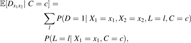and thus the condition 𝔼[D₁₁ – D₁₀ – D₀₁|C = c] > 0 can be expressed as

where p_x1x2lc = P(D = 1|X₁ = x₁,X₂ = x₂,L = l,C = c) and r_x1c(l) = P(L = l|X₁ = x₁,C = c).

Similarly, if the effects of X₁ and X₂ on D are monotonic, then 𝔼[D₁₁ – D₁₀ – D₀₁ + D₀₀|C = c] > 0 implies there must be some individual ω for whom D₁₁(ω) – D₁₀(ω) – D₀₁(ω) + D₀₀(ω) > 0 and thus there is a sufficient cause interaction. The condition 𝔼[D₁₁ – D₁₀ – D₀₁ + D₀₀|C = c] > 0 can be rewritten by using the g-formula as

If C and L consist of a small number of binary or categorical variables, then these conditions could potentially be tested for all strata of C. However, often C or L may consist of a large number of variables or may include continuous variables, so these conditions will be of limited use in practice. However, the approach for testing for sufficient cause interactions by using marginal structural models described in the text will still be applicable.

For n-way interactions, VanderWeele (11) showed that if there were an individual for whom

then there was an n-way sufficient cause interaction between the variables X₁, …, X_n. Thus, if for some baseline covariates L₁ we had a value l₁ such that

(A1)

then a sufficient cause interaction between the variables X₁, …, X_n must be present.

Suppose that there were sets of covariates L₁, …, L_n such that for i = 1, …, n,

where ${\stackrel{-}{X}}_{i-1}=(X_1,\mathrm{\dots },X_{i-1})$ and ${\stackrel{-}{L}}_i=(L_1,\mathrm{\dots },L_i)$. Then, by the g-formula, we would have that

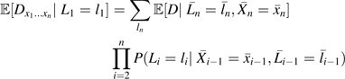(A2)

and we could test model 8 by using the empirical expressions in the right-hand side of A2.

VanderWeele (11) also gave counterfactual conditions for n-way sufficient cause interactions when either all or some subset of X₁, …, X_n had positive monotonic effects on D and these conditions could also be tested by using the empirical expression in A1.

APPENDIX 2

Prevalence Bounds for Sufficient Cause Interactions

A sufficient cause interaction is present for individual ω if D₁₁(ω) – D₁₀(ω) – D₀₁(ω) > 0 or, equivalently, since D₁₁, D₁₀, D₀₁ are binary, if D₁₁(ω) – D₁₀(ω) – D₀₁(ω) = 1. The quantity D₁₁(ω) – D₁₀(ω) – D₀₁(ω) can at most take the value 1 but can take a value as low as –2. From this it follows that for any variable Q, 𝔼[D₁₁ – D₁₀ – D₀₁|Q = q] will be a lower bound on the prevalence of individuals with Q = q for whom D₁₁(ω) – D₁₀(ω) – D₀₁(ω) = 1, that is, for whom a sufficient cause interaction is present. If Q is chosen as the empty set, then it follows that 𝔼[D₁₁ – D₁₀ – D₀₁] will be a lower bound on the prevalence of individuals in the population for whom a sufficient cause interaction is present. The quantity 𝔼[D₁₁ – D₁₀ – D₀₁|Q = q] will not in general be equal to the prevalence of individuals with Q = q for whom D₁₁(ω) – D₁₀(ω) – D₀₁(ω) = 1 since D₁₁(ω) – D₁₀(ω) – D₀₁(ω) may take negative values for some ω.

Similarly, under monotonicity, a sufficient cause interaction is present for individual ω if D₁₁(ω) – D₁₀(ω) – D₀₁(ω) + D₀₀(ω) = 1; under monotonicity, D₁₁(ω) – D₁₀(ω) – D₀₁(ω) + D₀₀(ω) will be at most 1 and at least –1. For any variable Q, 𝔼[D₁₁ – D₁₀ – D₀₁ + D₀₀|Q = q] will be a lower bound on the prevalence of individuals with Q = q for whom a sufficient cause interaction is present. If Q is chosen as the empty set, then it follows that 𝔼[D₁₁ – D₁₀ – D₀₁ + D₀₀] will be a lower bound on the prevalence of individuals in the population for whom a sufficient cause interaction is present.

Because the prevalence of sufficient cause interaction cannot be less than 0, it follows that max(0, 𝔼[D₁₁ – D₁₀ – D₀₁|Q = q]) and max(0, 𝔼[D₁₁ – D₁₀ – D₀₁ + D₀₀|Q = q]) constitute lower bounds on the prevalence of sufficient cause interactions in the stratum Q = q, without and with the monotonicity assumption, respectively. From this, it also follows that

and

will constitute lower bounds on the population prevalence of sufficient cause interactions without and with the monotonicity assumption, respectively. In general, these bounds will be larger than the crude bounds given by 𝔼[D₁₁ – D₁₀ – D₀₁] or 𝔼[D₁₁ – D₁₀ – D₀₁ + D₀₀].

A further point concerning interpretation is worth noting. In a recent paper, Hoffmann et al. proposed a method to estimate a quantity, PDC, representing “the proportion of disease due to a class of sufficient causes” (20, p. 77). Because the attributable fraction formulas used by Hoffmann et al. correspond to the proportion of diseased subjects who would not develop the disease if certain exposures were eliminated, it follows that the formula Hoffmann et al. give for “the proportion of disease due to a class of sufficient causes” should not in fact be interpreted as the proportion “due to” a specific sufficient cause but rather as the proportion that “could be eliminated by blocking the effect of” a specific sufficient cause. The distinction is subtle but important and can be seen clearly by a simple example.

Suppose that an individual had 2 sufficient causes completed, A₁X₁ and A₅X₁X₂. Suppose the outcome is death by time t^*. Suppose furthermore that the sufficient cause A₁X₁ leads to death at time t₁ < t^*, whereas the sufficient cause A₅X₁X₂ leads to death at time t₀ < t₁ < t^*. Since the individual has both sufficient causes, the individual dies at time t₀ from the sufficient cause A₅X₁X₂. The death is “due to the sufficient cause S = A₅X₁X₂.” However, if the sufficient cause A₅X₁X₂ is prevented from operating, the individual will still die from sufficient cause A₁X₁. Thus, the actual death is due to the sufficient cause A₅X₁X₂ but cannot be prevented by blocking just the sufficient cause A₅X₁X₂. The calculation of Hoffmann et al. (20) for the PDC for S = A₅X₁X₂ does not include this person in the numerator of the proportion and thus captures “the proportion of diseased subjects who would not develop the disease if a specific sufficient cause could be prevented from operating” rather than “the proportion of diseased subjects who develop the disease due to a specific sufficient cause.” Greenland and Robins (31) discuss attributable fractions (32) and distinguish between an “excess fraction” and an “etiologic fraction.” Essentially, the quantities discussed by Hoffmann et al. correspond to what Greenland and Robins define as the “excess fraction,” whereas the presence of a sufficient cause interaction indicates, in the terminology of Greenland and Robins, that there is a nonzero “etiologic fraction.” These observations generalize to the case of sufficient causes the distinction that Greenland and Robins draw between “excess fractions” and “etiologic fractions” for individual component causes. The true etiologic fraction for a specific sufficient cause is not in general identified, but, in related work, we have derived bounds for this proportion; refer to VanderWeele (33) for further discussion of attributable fractions for sufficient causes.

References

- 1.Rothman KJ. Causes. Am J Epidemiol. 1976;104(6):587–592. doi: 10.1093/oxfordjournals.aje.a112335. [DOI] [PubMed] [Google Scholar]
- 2.VanderWeele TJ, Robins JM. Empirical and counterfactual conditions for sufficient cause interactions. Biometrika. 2008;95(1):49–61. [Google Scholar]
- 3.VanderWeele TJ, Robins JM. The identification of synergism in the sufficient-component-cause framework. Epidemiology. 2007;18(3):329–339. doi: 10.1097/01.ede.0000260218.66432.88. [DOI] [PubMed] [Google Scholar]
- 4.VanderWeele TJ. Sufficient cause interactions and statistical interactions. Epidemiology. 2009;20(1):6–13. doi: 10.1097/EDE.0b013e31818f69e7. [DOI] [PubMed] [Google Scholar]
- 5.Vansteelandt S, VanderWeele TJ, Tchetgen E, et al. Multiply robust inference for statistical interactions. J Am Stat Assoc. 2008;103(484):1693–1704. doi: 10.1198/016214508000001084. [DOI] [PMC free article] [PubMed] [Google Scholar]
- 6.VanderWeele TJ, Hernán MA. From counterfactuals to sufficient component causes and vice versa. Eur J Epidemiol. 2006;21(12):855–858. doi: 10.1007/s10654-006-9075-0. [DOI] [PubMed] [Google Scholar]
- 7.Robins JM, Hernán MA, Brumback B. Marginal structural models and causal inference in epidemiology. Epidemiology. 2000;11(5):550–560. doi: 10.1097/00001648-200009000-00011. [DOI] [PubMed] [Google Scholar]
- 8.Robins JM. Marginal structural models versus structural nested models as tools for causal inference. In: Halloran ME, Berry D, editors. Statistical Models in Epidemiology: The Environment and Clinical Trials. Vol 16. New York, NY: Springer-Verlag; 1999. pp. 95–134. [Google Scholar]
- 9.Greenland S, Poole C. Invariants and noninvariants in the concept of interdependent effects. Scand J Work Environ Health. 1988;14(2):125–129. doi: 10.5271/sjweh.1945. [DOI] [PubMed] [Google Scholar]
- 10.Greenland S, Brumback B. An overview of relations among causal modelling methods. Int J Epidemiol. 2002;31(5):1030–1037. doi: 10.1093/ije/31.5.1030. [DOI] [PubMed] [Google Scholar]
- 11.VanderWeele TJ. Contributions to the Theory of Causal Directed Acyclic Graphs [doctoral thesis] Cambridge, MA: Harvard University; 2006. [Google Scholar]
- 12.VanderWeele TJ, Robins JM. Minimal sufficient causation and directed acyclic graphs. Ann Stat. 2009;37(3):1437–1465. [Google Scholar]
- 13.Rothman KJ, Greenland S, Lash TL, editors. Modern Epidemiology. 3rd ed. Philadelphia, PA: Lippincott Williams & Wilkins; 2008. [Google Scholar]
- 14.Robins JM. A new approach to causal inference in mortality studies with sustained exposure period—application to control of the healthy worker survivor effect. Math Model. 1986;7:1393–1512. [Google Scholar]
- 15.Robins JM. Addendum to a new approach to causal inference in mortality studies with sustained exposure period—application to control of the healthy worker survivor effect. Comput Math Appl. 1987;14:923–945. [Google Scholar]
- 16.Cole SR, Frangakis CE. The consistency statement in causal inference: a definition or an assumption? Epidemiology. 2009;20(1):3–5. doi: 10.1097/EDE.0b013e31818ef366. [DOI] [PubMed] [Google Scholar]
- 17.VanderWeele TJ. Concerning the consistency assumption in causal inference. Epidemiology. 2009;20(6):880–883. doi: 10.1097/EDE.0b013e3181bd5638. [DOI] [PubMed] [Google Scholar]
- 18.Cole SR, Hernán MA. Constructing inverse probability weights for marginal structural models. Am J Epidemiol. 2008;168(6):656–664. doi: 10.1093/aje/kwn164. [DOI] [PMC free article] [PubMed] [Google Scholar]
- 19.VanderWeele TJ. Sufficient cause interactions for categorical and ordinal exposures with three levels. Biometrika. In press doi: 10.1093/biomet/asq030. [DOI] [PMC free article] [PubMed] [Google Scholar]
- 20.Hoffmann K, Heidemann C, Weikert C, et al. Estimating the proportion of disease due to classes of sufficient causes. Am J Epidemiol. 2006;163(1):76–83. doi: 10.1093/aje/kwj011. [DOI] [PubMed] [Google Scholar]
- 21.Ahsan H, Chen Y, Parvez F, et al. Health Effects of Arsenic Longitudinal Study (HEALS): description of a multidisciplinary epidemiologic investigation. J Expo Sci Environ Epidemiol. 2006;16(2):191–205. doi: 10.1038/sj.jea.7500449. [DOI] [PubMed] [Google Scholar]
- 22.Chen Y, Graziano JH, Parvez F, et al. Modification of risk of arsenic-induced skin lesions by sunlight exposure, smoking, and occupational exposures in Bangladesh. Epidemiology. 2006;17(4):459–467. doi: 10.1097/01.ede.0000220554.50837.7f. [DOI] [PubMed] [Google Scholar]
- 23.VanderWeele TJ. On the distinction between interaction and effect modification. Epidemiology. 2009;20(6):863–871. doi: 10.1097/EDE.0b013e3181ba333c. [DOI] [PubMed] [Google Scholar]
- 24.VanderWeele TJ. Epistatic interactions [electronic article] Stat Appl Genet Mol Biol. In press doi: 10.2202/1544-6115.1517. [DOI] [PMC free article] [PubMed] [Google Scholar]
- 25.Khoury MJ, Flanders WD. Nontraditional epidemiologic approaches in the analysis of gene-environment interaction: case-control studies with no controls! Am J Epidemiol. 1996;144(3):207–213. doi: 10.1093/oxfordjournals.aje.a008915. [DOI] [PubMed] [Google Scholar]
- 26.Greenland S, Neutra R. Control of confounding in the assessment of medical technology. Int J Epidemiol. 1980;9(4):361–367. doi: 10.1093/ije/9.4.361. [DOI] [PubMed] [Google Scholar]
- 27.Rosenbaum PR. The consequences of adjustment for a concomitant variable that has been affected by the treatment. J R Stat Soc (A) 1984;147:656–666. [Google Scholar]
- 28.Robins JM, Morgenstern H. The foundations of confounding in epidemiology. Math Model. 1987;14:869–916. [Google Scholar]
- 29.Robins J. The control of confounding by intermediate variables. Stat Med. 1989;8(6):679–701. doi: 10.1002/sim.4780080608. [DOI] [PubMed] [Google Scholar]
- 30.Weinberg CR. Toward a clearer definition of confounding. Am J Epidemiol. 1993;137(1):1–8. doi: 10.1093/oxfordjournals.aje.a116591. [DOI] [PubMed] [Google Scholar]
- 31.Greenland S, Robins JM. Conceptual problems in the definition and interpretation of attributable fractions. Am J Epidemiol. 1988;128(6):1185–1197. doi: 10.1093/oxfordjournals.aje.a115073. [DOI] [PubMed] [Google Scholar]
- 32.Miettinen OS. Proportion of disease caused or prevented by a given exposure, trait or intervention. Am J Epidemiol. 1974;99(5):325–332. doi: 10.1093/oxfordjournals.aje.a121617. [DOI] [PubMed] [Google Scholar]
- 33.VanderWeele TJ. Attributable fractions for sufficient career interactions. Int J Biostat. doi: 10.2202/1557-4679.1202. In press. [DOI] [PMC free article] [PubMed] [Google Scholar]
Associated Data
This section collects any data citations, data availability statements, or supplementary materials included in this article.