Rapid Likelihood Analysis on Large Phylogenies Using Partial Sampling of Substitution Histories

Abstract

Likelihood-based approaches can reconstruct evolutionary processes in greater detail and with better precision from larger data sets. The extremely large comparative genomic data sets that are now being generated thus create new opportunities for understanding molecular evolution, but analysis of such large quantities of data poses escalating computational challenges. Recently developed Markov chain Monte Carlo methods that augment substitution histories are a promising approach to alleviate these computational costs. We analyzed the computational costs of several such approaches, considering how they scale with model and data set complexity. This provided a theoretical framework to understand the most important computational bottlenecks, leading us to combine novel variations of our conditional pathway integration approach with recent advances made by others. The resulting technique (“partial sampling” of substitution histories) is considerably faster than all other approaches we considered. It is accurate, simple to implement, and scales exceptionally well with dimensions of model complexity and data set size. In particular, the time complexity of sampling unobserved substitution histories using the new method is much faster than previously existing methods, and model parameter and branch length updates are independent of data set size. We compared the performance of methods on a 224-taxon set of mammalian cytochrome-b sequences. For a simple nucleotide substitution model, partial sampling was at least 10 times faster than the PhyloBayes program, which samples substitutions in continuous time, and about 100 times faster than when using fully integrated substitution histories. Under a general reversible model of amino acid substitution, the partial sampling method was 1,600 times faster than when using fully integrated substitution histories, confirming significantly improved scaling with model state-space complexity. Partial sampling of substitutions thus dramatically improves the utility of likelihood approaches for analyzing complex evolutionary processes on large data sets.

Introduction

Molecular evolutionary analyses have traditionally been limited by the need for deeply sampled sequence data sets and by the high computational burden of likelihood-based phylogenetic methods. This situation is rapidly changing, however, creating the prospect that fundamental questions about the evolutionary process at the molecular-genetic level that were previously inaccessible can soon be addressed. Data limitations are disappearing with technological advancements that have led to increasingly cost-effective high-throughput DNA-sequencing methodologies. The number of completely sequenced vertebrate mitochondrial genomes, for instance, has risen from 67 in 2000 (Pollock et al. 2000) to almost 900 today. Even more impressive, as many as 43 vertebrate nuclear genomes have been sequenced well enough to generate substantially complete assemblies and gene builds in the past few years alone (Hubbard et al. 2009), and it is expected that most of these will be completely sequenced with next-generation technologies in the next year or so. Single molecule DNA-sequencing technologies should also soon become viable, and based on expectations for this technology, plans have begun on a 10,000 vertebrate genome project (genome10k.soe.ucsc.edu).

Although improving, the computational burden of likelihood-based phylogenetic methods has not decreased as fast as the size of data sets has increased, and this burden is becoming more of an impediment as data sets grow and models become more complex. Part of the problem is that standard computations for continuous-time Markov chains (CTMCs) have components that scale in complexity with the second, third, and even fourth powers of the number of modeled states. Such poor scaling means that these techniques do not translate well from, for example, nucleotide substitution models with four states to amino acid substitution models with 20 states, codon-substitution models with 61 (sense) states, or to “switching models” that allow variation in the substitution process over time (e.g., Guindon et al. 2004) and effectively have much larger state spaces. Standard phylogenetic likelihood calculations also tend to scale poorly with increasing numbers of taxa, which is unfortunate because understanding the evolutionary process at individual sites requires dense taxonomic sampling (e.g., Pollock et al. 2000). Despite recent progress in the development of methods for rigorous inference under complex models or large data sets (Robinson et al. 2003; Hwang and Green 2004; Krishnan et al. 2004; Siepel and Haussler 2004; Mateiu and Rannala 2006; Rodrigue et al. 2006, 2007, 2008; Saunders and Green 2007; de Koning et al. 2009), substantial challenges remain.

Traditional maximum likelihood (ML) and Bayesian phylogenetic approaches are computationally demanding primarily because for every site in a sequence alignment they integrate every likelihood function evaluation over the typically huge space of all possible combinations of unknown ancestral states and all possible unknowable substitution histories. These integrations may be performed thousands of times or more in a typical analysis, so the vast majority of computations are spent repeatedly solving and resolving these integrals. Markov chain Monte Carlo (MCMC) and expectation–maximization methods can solve these integrals using data augmentation (DA; see Little and Rubin 2002; Rodrigue et al. 2007 for reviews), thus reducing the computational burden of likelihood-based analyses and increasing the complexity of models that may be practically considered. In particular, the recent introduction of techniques for augmenting substitution histories (or “mutation mappings”) (Nielsen 2002; Robinson et al. 2003; Hwang and Green 2004; Rodrigue et al. 2008) has led to tremendous performance improvements (Lartillot 2006). The primary advantage of these approaches is that when the timings of substitutions are fixed, the likelihood of the joint set of observed sequences and the augmented substitution history is much easier to evaluate than is the fully integrated form. Even after accounting for the need to run Markov chains for more generations when augmenting than when not, the net gain in efficiency can be huge. Sampling ancestral states and substitution histories, however, remains a costly computational step and is a key performance bottleneck for such approaches.

Here, we present a theoretical analysis and discussion of the computational costs of different augmentation strategies and then evaluate how these costs change with dimensions of model and data set complexity. Using this analysis, we show how the efficiency of sampling substitution histories can be dramatically improved without incurring a meaningful loss in accuracy. We show that the resulting method is easy to implement, accurate, and extremely fast, and we compare its performance with a variety of other approaches using a large data set of mammalian cytochrome-b sequences. For those readers less interested in the computational details, we recommend skipping over the Computational Considerations and Methods sections and moving directly to the Results section, where we reiterate the major conceptual points of those sections.

Computational Considerations

To identify and reduce the computational bottlenecks associated with conducting augmented likelihood analyses, we performed a theoretical analysis of the computational effort required by alternative phylogenetic likelihood calculations (the “time complexity,” or “order”). To quantify computational burden, we use a form of “big O” notation (Cormen 2009) to describe how time complexity scales with dimensions of the model and the input data, including the number of states in the evolutionary model (N), the number of branches in the tree (B), and the number of unique site patterns in the multiple sequence alignment (s). Because the order calculations are expressed as a function of each of these dimensions, readers familiar with time complexity analysis are cautioned to not assume that N has any special importance beyond being one of several dimensions of interest. For transparency, time complexity statements are presented in an expanded form, with separate terms given for each nontrivial component calculation.

Full Integration

Traditional ML and Bayesian phylogenetic methods integrate each likelihood function evaluation over both ancestral states and substitution histories. Ancestral states are usually integrated using Felsenstein's pruning algorithm (Felsenstein 1981); this technique follows a postorder traversal over the tree (from tips to root) at every site, where the likelihoods of all data below the current node are calculated, conditional on each possible state assignment (the “conditional site likelihoods”). Although this is known to be an efficient solution, the size of the problem still makes it time consuming. Pruning is an $\text{O}\left(N^{2}Bs\right)$ procedure, because $\text{O}\left(N^2\right)$ combinations of ancestral and descendent states must be considered at each internal node, O(B), for every site pattern, O(s). This calculation can therefore be quite costly for data sets with many taxa or long sequences or when complex models with many states are used. Even worse, because the time complexity of the pruning step scales multiplicatively with each dimension, combinations of long sequences, deep taxonomic sampling, and complex models can slow the operation, and it often dominates the time complexity of fully integrated likelihood calculations as a result.

Unlike integration over ancestral states, substitution histories are usually integrated implicitly along each branch by solving for the time-dependent substitution probabilities under a CTMC:

(1)

where P(t) is the matrix of substitution probabilities over branch length t, and Q is the matrix of instantaneous rates. This matrix exponential equation arises as the solution to the Chapman forward equation, which integrates over all possible substitutions having happened at all possible times (Ross 2007). Because this integration must be performed for many branches, equation (1) is usually solved by spectral decomposition of the rate matrix, allowing P(t) to be efficiently calculated for many t‘s (Moler and Van Loan 2003). Although spectral decomposition can be performed efficiently using well-known methods, the underlying matrix computations are often still relatively costly, incurring O(N₄) operations for the spectral decomposition of a nonreversible model (or O(N₃) for a reversible model), plus O(N₃B) operations to calculate the substitution probability matrices for every branch in the tree. Note that for simplification, we represent the cost of finding all eigenvalues and eigenvectors of a real non-symmetric matrix using the approximate worst-case cost of O(N₄), even though algorithms exist that can solve this problem in approximately O(30N₃) time (Golub and Van Loan, 1996).

We will subsequently refer to the integration over substitution histories as the “time integration” of the Markov process and the joint integration over both ancestral states and substitution histories as “full integration.” The likelihood function used in full integration is known as the “incomplete data” likelihood, where “incomplete” refers to the missing data (the unobserved ancestral states and substitution histories), which are fully integrated over. Combining the time complexity of both steps described above, the time complexity of an incomplete-data likelihood function is $\text{O}(N^4+N^{3}B+N^{2}Bs)$ operations (table 1, row 1).

Table 1.

Computational Time Complexity^a of Alternative Phylogenetic Likelihood Calculations.

			Time Complexity of
	Ancestral States	Substitution Histories	Likelihood Function	Missing Data Gibbs Sampler
1	Fully integrated	Fully integrated	$\text{O}\left(N^4+N^{3}B+N^{2}Bs\right)$	n/a
2	Sampled	Fully integrated	$\text{O}\left(N^4+N^{3}B+N^{2}B\right)$	$\text{O}\left(N^4+N^{3}B+N^{2}Bs+NBs\right)$
3a	Sampled	Fully sampled in continuous time (Nielsen 2002)	O(N2)	$\text{O}\left(N^4+N^{3}B+N^{2}Bs+NBs+NB\stackrel{-}{\mu }s{X}_1\right)$
b		Fully sampled in continuous time (Rodrigue et al. 2008)	O(N2)	$\text{O}\left(N^4+N^{3}B+N^{2}Bs+NBs+NB\stackrel{-}{\mu }s+N^3{X}_2\right)$
4	Sampled	Fully sampled in discrete time (Hwang and Green 2004)	O(N2)	$\text{O}\left(N^2+N^2{B^{\prime }}_{1}s+N{B^{\prime }}_{1}s\right)$, B  ≪ B‘1
5a	Sampled	Integrated assuming ≤ 2 substitutions, ‘B2’ CP (Krishnan et al. 2004; de Koning et al. 2009)	$\text{O}\left(N^{3}B+N^{2}B\right)$	$\text{O}{\left(N^{3}B+NBs\right)}^{}$b
b		Integrated assuming ≤1 substitutions, “B1” CP (Krishnan et al. 2004)	$\text{O}\left(N^{2}B+N^{2}B\right)$	$\text{O}{\left(N^{2}B+NBs\right)}^{}$b
6	Sampled	Partially sampled: branch segmentation with B1 CP (“‘B1 × M”’; present study)	O(N2)	$\text{O}\left(N^2+N^2{B^{\prime }}_{2}s+N{B^{\prime }}_{2}s\right)$, $B\ll {B^{\prime }}_2<{B^{\prime }}_1$
7a	Sampled	Partially sampled: long-branch bisection with uniformized B1 CP (“B1u‘” present study)	O(N2)	$\text{O}\left(N^2{B^{\prime }}_3+N^2{B^{\prime }}_{3}s+N{B^{\prime }}_{3}s\right)$, $B\le {B^{\prime }}_3\ll {B^{\prime }}_2<{B^{\prime }}_1$
b		Partially sampled: long-branch bisection with uniformized B1 CP (“B1u”; present study)	O(N2)	$\text{O}\left(N{B^{\prime }}_{3}s\right)$b, $B\le {B^{\prime }}_3\ll {B^{\prime }}_2<{B^{\prime }}_1$

^aThe approximate number of operations are given in terms of: N = num. modeled states, B = num. branches in the tree (or effective branches, B′), s = num. unique site patterns in the data, $\stackrel{-}{\mu }$ = average num. substitutions per branch, X₁ = average num. attempts before success, and X₂ = maximum num. substitutions per branch.

^bUsing the local Gibbs updater (Krishnan et al. 2004).

Sampling of Ancestral States and Substitution Histories

An alternative to full integration is to compute likelihoods after periodically filling in (or “augmenting”) some or all of the missing data with likely imputed values, sampled based on the model and its current parameter values (Gelman et al. 1992; Little and Rubin 2002). DA usually begins by drawing a state at the root of the tree from the product of the stationary distribution of the CTMC and the conditional site likelihoods. The states at all internal nodes are then drawn in a root-to-tip sequence from the conditional site likelihood distributions (Nielsen 2002). This method therefore requires both a pruning step and a sampling step, which can be performed together in $\text{O}(N^4+N^{3}B+N^{2}Bs+NBs)$ operations (table 1, row 2). Once ancestral states have been drawn, substitution histories can be sampled along each branch conditional on the fixed states at each pair of ancestral and descendant nodes (Nielsen 2002; Robinson et al. 2003). When both ancestral states and substitution histories are augmented along each branch, we will refer to this as “full sampling.”

Remarkably, when full substitution histories are sampled, the augmented likelihood function can be evaluated in as few as O(N₂) operations, no matter how many branches or sites are considered. This is because the substitution history can be equivalently represented by the numbers of each substitution type across the entire data set, along with the total time spent in each state without changing (Lartillot 2006) (i.e., by N₂ quantities that are sufficient statistics of the augmented data). In practical terms, the speed with which this augmented likelihood function can be evaluated is so rapid that methods that sample substitution histories tend to spend virtually all of their time resampling the missing data, even if the sampling step is performed infrequently.

There are currently several approaches in use for sampling substitution mappings along branches, which can be roughly divided into continuous and discrete-time methods (fig. 1a and b, respectively). Probably the most widely used of such approaches sample substitutions in continuous time (Nielsen 2002; Robinson et al. 2003; Rodrigue et al. 2008), although the performance of these methods is hindered by their need to perform the full time integration of the Markov process, a variety of costly matrix computations, and a number of subsequent sampling steps (table 1, rows 3a and 3b).

FIG. 1.

Strategies for sampling substitution histories. (a) Substitutions are fully sampled in continuous time using a method such as Nielsen (2002) or Rodrigue et al.(2008). (b) Substitutions sampled in discrete time over short-branch segments of equal length (Hwang and Green 2004). (c) Substitutions partially sampled in continuous time to within short time intervals of different lengths using B1 CP intregration (B1 × M). (d) Substitutions partially sampled in continuous time as ancestral and transient states at fixed points that bisect long branches; the timing of substitutions between nodes is analytically integrated using uniformized B1 CP integration (B1u). For both (b,c), branch lengths are rounded to the nearest small segment size.

Hwang and Green (Hwang and Green 2004) (HG, hereafter) introduced a discrete-time approach that achieves an augmented likelihood function of O(N₂) over the entire data set but that also leads to a simpler time integration of the Markov chain in the missing data sampler (table 1, row 4). This simplification is achieved by breaking branches into a series of short, equal-length segments (“branch segmentation,” hereafter) that are treated as discrete-time units and by approximating branch lengths as a discrete number of these segments (fig. 1b). With only one branch length, there is only one set of substitution probabilities to calculate (eliminating a branch-dependent O(N₃B) term in time integration), and spectral decomposition is no longer required (eliminating an O(N₄) term compared with time integration). By using a segment length that is small enough to be considered “effectively infinitesimal” (e.g., t = 0.005), substitution probability calculations can be further simplified by considering that

(2)

for small t, thus implying

(3)

This approach therefore replaces the costly time integration of continuous-time approaches with a comparatively trivial O(N₂) calculation.

In the HG approach, the complete substitution history (in discrete time) is sampled using Nielsen's algorithm for sampling ancestral states (Nielsen 2002), except that the algorithm is applied to all branch segments (B′), rather than to whole branches (B). The time complexity of the missing data sampler is therefore $\text{O}(N^2+N^{2}B\prime s+NB\prime s).$ Unfortunately, because the approximation in equation (3) and the rounding of branch lengths require that a short branch segment size be used, B′ will often be quite large. This causes a major problem, in that the efficiency gained by avoiding time integration is offset by the increased cost of having a larger number of branch segments. We have found that, in practice, the size of B′ sometimes leads to a net loss in performance compared with other approaches as a result (data not shown). As we show later, the HG segmentation approach also increases the time for the Markov chain to reach equilibrium, further exacerbating its computational burden.

Partial Sampling of Substitution Histories with Conditional Pathway Integration

We previously introduced several continuous-time conditional pathway (CP) integration methods (Krishnan et al. 2004; de Koning et al. 2009) that augment ancestral states and condition substitution probability calculations on no more than one or two substitutions having occurred along a branch at each site (B1 and B2, respectively). These methods facilitate relatively inexpensive augmented likelihood functions and missing data samplers by ignoring large numbers of improbable intermediate substitution pathways and simplifying the time-integration of the Markov process as a result (table 1, rows 5a and 5b). In our original presentation of these methods, we recommended using a branch subdivision strategy to ensure that each branch segment is kept short enough that the B1 or B2 assumptions remain appropriate. Here, we explore several such strategies and describe how they can be combined with novel CP variants to produce high performance methods that overcome performance bottlenecks of the methods discussed so far.

In the methods presented below, we use both a variation on branch segmentation (in Method 1) and a strategy where long branches are successively broken in half until all segments are shorter than a specified threshold (“long-branch bisection”; in Method 2). An important feature of long-branch bisection is that the maximum allowed branch length provides a convenient control point that can be manipulated to achieve desired precision versus speed trade-offs. When a reasonable value is used for this parameter, the number of effective branches is much smaller than with segmentation methods and is typically only slightly larger than the total number of actual branches.

We refer to both of these approaches as “partial sampling” or “partial integration” techniques, because breaking branches in the continuous-time case is equivalent to introducing fixed time points along branches at which the transient states of the CTMC will be sampled. In this way, substitutions are sampled to the nearest branch segment with the timing of events analytically integrated within segments, thus achieving a faithful representation of the full CTMC. Due to the continuous-time formulation, we expect to obtain more accurate parameter estimates than under discrete-time methods such as HG (a prediction we examine below). Despite this, these approaches are nearly as simple to implement as HG because they require no special steps to sample the substitution history per se and thereby allow ancestral and transient states to be sampled together in the same process.

Method 1: Branch Segmentation in Continuous Time (“B1 × M”)

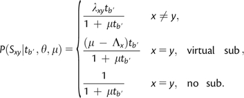
The first newly introduced method uses branch segmentation but with analytical CP integration over the timing of events within segments using B1 (fig. 1c). If a branch segment of length $t_{b\prime }$ is short enough that the probability of >1 substitution is negligible, the substitution probability can be well approximated by assuming no more than 1 event (Krishnan et al. 2004). By integrating this calculation over all possible timings of the event within a branch, the B1 CP substitution probability is obtained exactly as

(4)

where S_xy is the substitution from state x to y, ${\lambda }_{xy}$ is the rate parameter governing the instantaneous rate of substitution from x to y, ${\mathit{\Lambda }}_x$ is the sum of substitution rates from x to any different state, and θ is the set of all rate parameters (Krishnan et al. 2004).

Using equation (4), the approximation in equation (3) is no longer needed, and longer branch segments can be used without sacrificing accuracy (also examined empirically below). This allows the number of effective branches to be greatly reduced, helping to overcome the major performance hurdle of HG. To keep the approximation of total branch lengths accurate, a small number of additional (shorter) segment sizes can be used at the ends of branches without reducing computational speed very much. As in HG, there is therefore only one segment size (or just a few), and thus only one substitution probability matrix (or just a few) to calculate for the entire tree. As well as having several advantages over HG, this technique of B1 with branch segmentation (B1 × M) is expected to be more accurate than standard B1, because the average segment length will be much shorter than the average branch length.

Considering the time complexity of B1 × M (table 1, row 6) compared with time integration, the $\text{O}\left(N^4\right)$ spectral decomposition term is eliminated and the $\text{O}\left(N^{3}B\right)$ calculation of substitution probability matrices is simplified to $\text{O}\left(N^2\right)$ due to equation (4) and because there is only one branch length (or just a few). The time complexity of the missing data sampler under B1 × M is $\text{O}(N^2+N^2{B}^{\prime }s+N{B}^{\prime }s),$ as in HG's method, but $B^{\prime }$ can be much smaller while maintaining equivalent accuracy. This improves the computational speed and greatly reduces the time for the Markov chain to reach equilibrium compared with HG.

Method 2: Uniformized B1 (“B1u”) with Long-Branch Bisection

Although B1 × M is expected to be much faster than HG, some problems remain. First, $B^{\prime }$ can still be quite a bit larger than B, adding to the burden of the missing data sampler. Second, B1 × M still requires that total branch lengths be rounded to the nearest segment length, creating some approximation error. These limitations are overcome with the second newly introduced method, which is based on a rederivation of the B1 substitution probability using uniformization, combined with a long-branch bisection strategy (B1u, hereafter; fig. 1d).

When the waiting times for substitutions from the beginning and ending states on a branch, x and y, are equal, the B1 calculations in equation (4) simplify to

(5)

where $\mu ={\mathit{\Lambda }}_x={\mathit{\Lambda }}_y.$ One can imagine that if μ were made independent of the rate parameter ${\lambda }_{xy}$ (normally it is not), then the rate parameter term and the branch-length terms would be separable. As described in detail in Methods, the uniformization technique (Ross 2007) allows this independence to be achieved in practice. A key outcome of separating the rate and branch terms is that it leads to a useful simplification of the likelihood function. Using uniformization, the augmented likelihood function can be written in such a way that all rate parameters can be updated in $\text{O}\left(N^2\right)$ operations and all branch lengths can be updated in O(B) operations. A single rate or branch-length parameter can be updated with O(1) performance. Importantly, these simplifications are achieved without requiring branch-length approximation, as in HG and B1 × M, and without requiring excessive segmentation, as in HG. This suggests that B1u should be both faster and more accurate than those approaches.

The strategy of using B1u with long-branch bisection not only leads to “best in class” augmented likelihood function performance (i.e., on par with continuous-time sampling and HG), but also to large improvements in the performance of the missing data sampler as well (table 1, row 7). Using long-branch bisection with “standard B1,” the missing data sampler requires $\text{O}(N^2{B}^{\prime }+N^2{B}^{\prime }s+N{B}^{\prime }s)$ operations, consisting of the calculation of all substitution probability matrices, a pruning step, and a sampling step. This can be further simplified to $\text{O}(N^2{B}^{\prime }+N{B}^{\prime }s)$ by adopting a local Gibbs updater that we introduced previously (Krishnan et al. 2004), which resamples ancestral states conditional on the current states at all surrounding nodes, starting at a randomly selected node and radiating outwards. This sampler appears to mix well with branch bisection (demonstrated below, although it mixes too slowly to be useful with branch segmentation approaches). With B1u, the time complexity of the local updater can be reduced even further to a mere $\text{O}\left(N{B}^{\prime }s\right)$ operations, because the change in likelihood caused by reassigning an ancestral or transient state can be calculated without needing to construct substitution probability matrices. Note that the order of this calculation is likely close to the minimum possible for any sampling strategy, because any such updater must sample from N possibilities, at each of Bs nodes and sites, for O(NBs) operations. The B1u performance of $\text{O}\left(N{B}^{\prime }s\right)$ is thus only slightly greater than the hypothetical optimum due to $B^{\prime }\mathrm{\ge }\mathit{B}\mathit{.}$

B1u therefore appears to have “best in class” performance because each of its component calculations is at least as efficient as any other method (as far as we are aware; table 1). In the following sections, we evaluate both B1 × M and B1u in comparison to standard methods and assess how variation in the amount of segmentation affects mixing and accuracy.

Methods

Likelihood Calculations

As outlined above, we propose several new CP integration approaches intended to reduce the time complexity of phylogenetic likelihood calculations as much as possible without incurring a meaningful loss in accuracy. Implementation details of these methods are provided below. Although these techniques are general and can be used with any CTMC-based evolutionary model (they work well with nonreversible models, for example), for the purposes of exposition, we use a simple general time reversible (GTR) model defined on either a nucleotide or amino acid state space. This choice is expected to be conservative in that the performance advantage of the new methods grows rapidly with increasing model complexity. Following Yang's convention (Yang 1994a, 2007) the rate of $A\leftrightarrow G$ substitutions was fixed to equal 1.0, and other substitution rates were measured relative to it.

Continuous-Time Branch Segmentation with CP Integration (B1 × M)

In the original version of the B1 CP method (Krishnan et al. 2004), a probability matrix had to be calculated for every branch because of the dependence of equation (4) on branch lengths; this yielded a likelihood function that is increasingly burdensome with more taxa. By instead approximating branches as a series of short, equal-length segments, an approximation to the full CTMC can be constructed wherein the timing of substitutions is integrated within each short segment using B1. This approach is similar in spirit to Hwang and Green's (Hwang and Green 2004) (HG) approach, but it provides a better approximation to the CTMC, while maintaining a fast $\text{O}\left(N^2\right)$ likelihood function over all sites and branches and using far fewer branch segments.

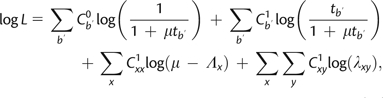
Because this approach is more accurate than HG, longer segments can be used to reduce the overall amount of segmentation while maintaining equivalent accuracy. To ensure that branch lengths are still approximated effectively, a small number of different segment sizes are used that include both long and short segments. Unless otherwise specified, analyses in this report use three segment sizes of 0.02, 0.01, and 0.005. Using this approach, the log-likelihood calculation across all sites for an augmented data set is

(6)

where $C_{xy,b^{\prime }}$ is the total number of branch segments of length $t_{b^{\prime }}$ (over all sites) upon which x changes to y, and

We refer to this approach as “B1 × M” in the text, where M reflects multiple segments per branch. Note that the $\log \left({\lambda }_{xy}\right)+\log \left({\kappa }_{xy}\right)$ calculation may need to be calculated for only a fraction of the state combinations, in part because the shorter branch segment lengths will sometimes have only a small probability that a change will have occurred on them, making some $C_{xy,b^{\prime }}$ zero.

A related approach “B∞xM” was also considered, which uses the fully integrated substitution probabilities instead of B1. In this way, the effects on likelihoods of segmentation and CP integration could be separately examined.

Long-Branch Bisection with Uniformized B1 CP Integration (B1u)

Under standard uniformization (Ross 2007), a CTMC is transformed so that the probability of leaving any state x is made the same, regardless of x. This uniform rate (the “uniformization rate” of total substitutions), μ, is achieved by introducing virtual substitutions from state x to state x that occur at a rate of $\mu -{\displaystyle {\sum }_j{\lambda }_{xj}=\mu -{\mathit{\Lambda }}_x}$ (where $j\mathrm{\ne }x$; see Ross 2007 for a detailed discussion). The uniformization rate must therefore be greater than or equal to the longest waiting time from the untransformed process, and the accuracy of the uniformization-based calculation is greatest when the uniformization rate is exactly equal to the longest waiting time $(\text{i}\text{.e}\text{.,}\mu =\underset{x}{\max }{\displaystyle {\sum }_j^{}{\lambda }_{xj}})$ Under these conditions, and under the B1 condition of ≤1 total substitutions, the probability of a particular substitution (including virtual substitutions) is ${\lambda }_{xy}{t}_{b\prime }{\text{e}}^{-\mu t_{b\prime }},$ and the probability of no substitutions (either real or virtual) is ${\text{e}}^{-\mu t_{b\prime }}.$ To find the probability of each substitution type out of the allowed types (i.e., ≤1 substitution per branch segment), each probability is divided by the sum of allowed substitutions, ${\text{e}}^{-\mu t_{b\prime }}+{\text{e}}^{-\mu t_{b\prime }}\mu t_{b\prime }.$ This normalization constant is found by taking the standard uniformization transition probability summation to n = 1 terms, which gives the Poisson probability of zero or one event in time $t_{b\prime }$ (Ross 2007).

The B1u substitution probabilities over a branch segment of length $t_{\text{b}\prime }$ after simplification by canceling out the ${\text{e}}^{-\mu t_{b\prime }}$ term and augmenting virtual substitutions are thus

(8)

The status of each x = y event can be augmented with an indicator variable simultaneously with the sampling of ancestral and transient states by drawing a random variate, $\upsilon ,$ from U(0,1) and labeling the event a virtual substitution if

(9)

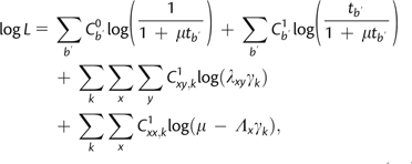
The log-likelihood calculation across all sites for a fully augmented data set (including the total numbers of virtual substitutions across the data set) can therefore be expressed as

(10)

where $C_{b^{\prime }}^0$ is the number of sites and branch segments of length $t_{b^{\prime }}$ with 0 substitutions, $C_{b^{\prime }}^1$ is the number with 1 substitution to anything (i.e., both virtual and real substitutions), $C_{xx}^1$ is the number with an xx virtual substitution, and $C_{xy}^1$ is the number with an xy substitution. Note that $b^{\prime }$ here is taken over the number of branches with different lengths. Because bisection entails breaking branches into a number of ultimately equal-length segments, however, $b^{\prime }$ is actually taken over only B terms, which is the number of unbroken branches.

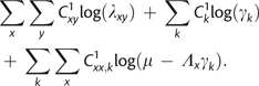
Because only the first two terms in equation (10) depend on branch lengths, the likelihood can be evaluated in $\text{O}\left(N^2\right)$ time once the ancestral and transient states are fixed (and the branch-dependent first and second terms are precomputed). Similarly, because only the last two terms in equation (10) depend on rate parameters, the B1u formulation allows for a simple change-in-likelihood function evaluation in O(1) time. Holding μ and the augmented data constant, the change in log-likelihood caused by altering a rate parameter ${\lambda }_{x,y}$ is

(11)

where $C_{xy}^1$ is the total number of sites and branch segments with 1 xy substitution (regardless of branch), $C_{xx}^1$ is the total number of sites and branch segments with 1 xx virtual substitution (regardless of branch), ${{\lambda }^{\prime }}_{xy}$ is the new (test) rate parameter to be changed, and ${\Lambda }_x^{\prime }$ is the updated sum of rate parameters from state x. The change in log-likelihood caused by altering a branch segment length from $t_{b^{\prime }}$ to ${t^{\prime }}_{b^{\prime }}$ is

(12)

In practice, additional considerations should be made when updating segment lengths to ensure that they do not exceed the defined maximum segment length (see Appendix).

The x = y terms in equation (8) could theoretically also be combined, thus eliminating the need to sample virtual substitutions. This, however, leads to a more complicated likelihood function having $\text{O}\left(N^2{B}^{\prime }\right)$ time complexity (just as the standard B1 method), because it would prevent the separation of rate and branch length terms for xx events. Nevertheless, integrating over virtual substitutions in this way can be used as a diagnostic check to examine how sampling virtual substitutions affects mixing performance.

MCMC Simulation

Individual MCMC simulations were run using a combination of Gibbs sampling (Geman S and Geman D 1984) over ancestral and transient states, and Metropolis Hastings updates (Metropolis et al. 1953; Hastings 1970) on rate parameters. Except where noted, branch lengths and the tree topology were held constant at their ML values. When branch lengths were considered free, they were sampled by a conjugate Gibbs approach for B1u (Appendix). Flat, uniform priors and symmetric proposal distributions were used throughout, so that the prior and proposal ratios canceled out in the Metropolis Hastings acceptance probability (as in Krishnan et al. 2004). Therefore, proposals were accepted with probability proportional to the likelihood ratio between current and proposed states. More sophisticated prior and proposal distributions can easily be used with our methods, but a focus on these distributions was not the aim of this work.

The variance of each proposal distribution was tuned using a simple adaptive mechanism based on an estimate of the posterior variance determined from a precalculated run of several hundred generations. When possible, simple analytical expressions for change-in-likelihoods were used to evaluate the acceptance probability of proposals (eqs. 11 and 12). Combined multidimensional proposals were also sometimes made, because they can move through high-dimensional space more rapidly than single parameter proposals, although they may be less efficient in general and have a lower optimal accept–reject ratio (Roberts et al. 1997).

When using B1u, a method for setting the uniformization rate, μ, is required. Although uniformization is valid for any value of $\mu \mathrm{\ge }{\max }_{\mathrm{x}}{\displaystyle {\sum }_j^{}{\lambda }_{xj}},$ it is most accurate when μ is as close to its bound as possible. Because updating μ can be computationally expensive, it is sometimes simply fixed at a value known to be greater than the largest possible waiting time under a priori model restrictions (Ross 2007). Here, we used an update mechanism to keep the uniformization rate close to its optimal value (Sandmann 2008). Over the course of an MCMC run, μ was therefore occasionally reset to ${\max }_{\mathit{x}}{\displaystyle {\sum }_j^{}{\lambda }_{xj}}+\sigma ,$ with σ set by experience to a small finite value.

Comparison of Time to Complete a Fixed Number of Generations of MCMC

Unless otherwise noted, all methods considered in the text were implemented in a common MCMC program so that the proposals and frequencies of different update types could be easily controlled and to limit implementation issues in method comparisons. An alignment of 224 mammalian cytochrome-b genes was used as a benchmark data set and was aligned in coding frame using a combination of POA (Lee et al. 2002; Grasso and Lee 2004) and Perl scripts. The cytochrome-b phylogeny was estimated under a GTR + Γ model by an ML heuristic search using all mitochondrial protein–coding genes from the same 224 species; the search was constrained to a consensus of ordinal relationships (Murphy et al. 2007) and run using PAUP* (Swofford 2003).

MCMC chains were run for 100,000 generations for each method, with 99.8% of updates on the GTR rate parameters and 0.2% on ancestral states (update proportions were determined empirically by reducing the frequency of ancestral state updates as much as possible without adversely affecting mixing). Branch lengths and tree topologies were held constant at their ML values for each run, whereas base frequencies were held constant at their mean observed values. The time to completion on a standard desktop computer (2.8-GHz Intel Core 2 Duo iMac) was recorded for comparison. Separately, the time to complete 100 ancestral state updates and 10,000 rate matrix updates was also recorded to examine the different costs these steps have across methods.

For the Full (fully integrated substitution histories), B1 × M, B∞xM, and HG methods, ancestral states were updated using the standard conditional site likelihood-based method (Nielsen 2002; Hwang and Green 2004). For B1 and B1u, we used the simpler local Gibbs sampler (Krishnan et al. 2004) that starts at a randomly selected node and resamples the states at each site conditional on the nodes immediately surrounding it. As discussed above, this updater has the advantage that it does not require conditional-site likelihoods to be calculated and therefore reduces the complexity of the most expensive part of ancestral state updates.

To determine if there were differences in mixing across methods, the effective sample size (ESS) of each chain after burn-in was calculated using R (R Core Development Team 2009) and the Coda package (Plummer et al. 2006). To estimate the amount of time required to achieve an average of 1,000 decorrelated posterior samples for each rate parameter, each analysis was run 10 times, and the mean generation times and ESSs were recorded.

Performance Comparison to Other Programs

We modified the MrBayes 3.2 (Huelsenbeck and Ronquist 2001; Ronquist and Huelsenbeck 2003) source code to disable its proposal mechanisms for tree topology and branch lengths, and set it to use empirical nucleotide frequencies and the same fixed tree topology and branch lengths as above. This resulted in MrBayes updating the GTR rate parameters 100% of the time, because it integrates each likelihood calculation over all possible ancestral states. Default prior probability distributions were used for all analyses. All source codes were compiled with the same compiler, using identical optimization settings. Time to complete 100,000 generations on the same computer was then used as a performance benchmark.

The number of generations sampled, however, has a different meaning among alternative methods and software implementations and is therefore not necessarily a fair means to make direct comparisons of performance. A consequence of this fact is that a program that completes many generations rapidly, but mixes poorly, might provide less informative data per unit time than an implementation that takes longer but mixes better. We therefore calculated the ESS after burn-in for each method as above and used differences in mixing efficiency to correct the actual (naïve) speed difference.

We also compared the speed of our implementation with an extremely fast Bayesian program, PhyloBayes 2.3c (Lartillot and Philippe 2004), which samples substitutions in continuous time (Rodrigue et al. 2008) and performs fast conjugate Gibbs sampling on rate parameters (Lartillot 2006). As with B1u, PhyloBayes spent virtually no measurable time performing rate parameter updates, as assessed from the monitor file output. Because resampling substitutions is the most time-consuming step in both methods, to be conservative, we considered only the time PhyloBayes spent in this step. Over a period of 100,000 generations, 200 updates of all transient and ancestral states were performed in our program. We therefore ran PhyloBayes for 100 cycles on the same data set, because by default it resamples substitutions twice each cycle. We could not fix branch lengths using PhyloBayes, so we did not evaluate its mixing performance in comparison to ours, although we expect it should be comparable due to the similarity of the methods.

Method Comparisons and Analysis

Average Probability of >1 Substitution for Random GTR Models.

The probability of greater than one substitution was calculated for increasing branch segment sizes using a modified version of the “evolver” program from PAML4 (Yang 2007). Fifty random GTR rate matrices were simulated for each branch length by sampling rate parameters from a uniform distribution, U ∼ (0,1], and normalizing the resulting matrix to sum to 1. Each CTMC was then transformed to a discrete-time Markov chain with standard uniformization (Ross 2007), allowing 1 minus the Poisson probability of ≤1 substitutions to be calculated.

Expected Error of HG and B1 with Increasing Segment Length.

To compare the expected error between HG and B1 with increasing branch-segment sizes, a simulation was performed using a modified version of evolver (Yang 2007) to approximate the expected error for each method. Fifty random GTR rate matrices were simulated for each branch length as above and were used to calculate the exact substitution probabilities using full-integration based on the matrix exponential. Rate parameters λ were calculated exactly for HG using $P\left(S_{xy}\right|t,\lambda )/t$ (eq. 2). Rate parameter values under B1 and B1u were found under an asymptotic approximation whereby we numerically minimized the root-mean squared difference (RMSD) between the B1 substitution probabilities and the exact substitution probabilities. The RMSD of the rate parameters were then calculated between the true simulated values and both of the HG and B1 values and were standardized by branch length. Mean and standard deviations at each branch-segment length were plotted on the same axis.

Predicted Speed Increase As a Function of the Number of Branches and Model States

To visualize how different approaches scale with increasing model and data set complexity, the predicted fold speed increase was plotted by taking the ratio of the time complexity of several methods (from table 1) compared with B1u over a range of parameter values expected to reflect a variety of analyses of interest. For comparison to the fastest published approach (sampling substitutions in continuous time), we assumed the use of the method of Rodrigue et al. (2008), with a maximum number of substitutions per branch set to 2, to be conservative about the speed improvement of B1u (analysis of the same data in PhyloBayes, yielded a maximum number of substitutions per branch at 7). For each approach, calculations were made for both reversible and nonreversible models, which were distinguished by a leading $\text{O}\left(N^4\right)$ term for nonreversible models and an $\text{O}\left(N^3\right)$ term for reversible ones.

Relative ML Support for Different Topologies

To generate a set of phylogenetic trees with which to compare the correspondence of relative likelihood support under Full and B1u, the 224 cytochrome-b data set was bootstrapped 10 times, and Neighbor-Joining trees were constructed for each pseudoreplicate using FastTree (Price et al. 2009). Each tree was rerooted using the monotremes as an outgroup. Branch-length estimates from FastTree were fixed and used to analyze the data using B1u and Full, as described above. The maximum attained incomplete-data log-likelihood following burn-in was recorded for each analysis and used to assess relative support. Each analysis was repeated while allowing branch lengths to be freely estimated, using the FastTree values as a starting point. ML values were compared between Full and B1u using linear regression analysis in R (R Core Development Team 2009).

Results

For readers who may have skipped the Computational Considerations and Methods sections, we provide the following summary: We carefully considered the theoretical basis of various likelihood-based phylogenetic methods to determine if their speed could be improved and whether they could be endowed with better scaling properties for large data sets and complex models of evolution. As a result, two new methods were introduced, merging our previous CP (Krishnan et al. 2004) approach with the most promising aspects of other approaches. These methods provide alternatives to sampling unknown substitution histories and making likelihood calculations on the basis of those histories. They use continuous-time approaches that partially sample the timing of substitutions to branch regions instead of to exact times and that integrate over the timing of substitutions within those regions. These new methods can therefore be thought of as sampling transient states of the evolutionary process at fixed time points along branches.

The first method, based on continuous-time branch segmentation, is called B1 × M. Here, B1 signifies integration over the timing of substitutions within branch segments using an approximation that assumes no more than one substitution per segment, and M signifies multiple segments per branch. The use of B1 × M allows for the number of segments to be reduced compared with the HG method (Hwang and Green 2004) without sacrificing accuracy and thus should improve the speed and mixing performance of the demanding process of resampling substitution histories.

Once B1 × M was developed, we realized that it only partially overcame the performance bottlenecks of previous approaches, and so we developed a second new approach using a rederivation of the B1 CP method based on uniformization (Ross 2007); we therefore refer to this second method as B1u. To keep the accuracy of B1u high, long branches are broken using long-branch bisection, allowing the maximum segment length to be adjusted to select among desired speed to precision trade-offs (longer maximum branch lengths lead to fewer segments and therefore faster computation but can be less precise).

The computational time of a method (the time complexity) responds to increases in model and data complexity as measured by the number of modeled states (N), the number of branches on the tree (B), and the number of site patterns in the nucleotide alignment (s). A time complexity analysis (table 1) predicted that B1u should theoretically be faster and scale better with model complexity and data-set size than any other method considered. The analyses presented in this section are designed to first consider the accuracy/branch length trade-offs with B1, then empirically evaluate the relative speed, mixing performance, accuracy, and precision of implementations of B1u and B1xM with alternative methods.

Predicted Rate Parameter Accuracy under Discrete- and Continuous-Time Branch Segmentation

Reasonable conditions for continuous-time branch segmentation and bisection were first evaluated by examining how long segments may reasonably be without violating the B1 assumption of one or fewer substitutions per branch segment. The average probability of >1 substitution was calculated for 50 random GTR rate matrices along branches of increasing lengths (fig. 2a). A segment as long as 0.08 was determined to have only about 0.5% probability of >1 substitution, whereas branch segments as short as 0.02 and 0.005 were seen to have a probability well below 0.05% and 0.01%, respectively. All such segment lengths were therefore deemed to represent reasonable approximations and were used in further investigations.

FIG. 2.

Validity and accuracy of methods assuming one substitution per branch segment. (a) The probability of more than one substitution per site with increasing branch segment size, calculated from the fully time-integrated Markov process. The mean ± standard deviation over 50 random GTR rate matrices is displayed for each segment size. (b) Approximate asymptotic expected error in rate parameters. Using the optimal uniformization constant, B1u is slightly more accurate than the standard B1 method (Krishnan et al. 2004), although both derivations give a similar result. Both B1 and B1u are much more accurate than HG, although they incur little additional computational expense.

To examine the theoretical accuracy of B1 × M compared with the related HG method, we performed a similar simulation to examine the relative error in rate parameters under asymptotic conditions for each method (fig 2b). Based on this analysis, B1 appeared to be approximately seven times more accurate than HG as measured by RMSD per unit time and was accurate even for relatively long segment sizes (also see supplementary fig. 1, Supplementary Material online).

Relative Speed and Mixing Performance of Continuous-Time B1 × M and B1u Implementations

A 224-taxon data set of mammalian cytochrome-b sequences (supplementary fig. 2, Supplementary Material online) was used as a benchmark data set and was analyzed using a GTR model with branch lengths and nucleotide frequencies fixed at their ML values. The time to complete equivalent analyses was used to assess performance (fig. 3). Performance varied across nearly two orders of magnitude, with B1u completing in 11 s what took 16.6 min using fully integrated probability calculations (“Full”)—a speedup of more than 90-fold. The time to complete the same analysis using B1u with the more expensive ancestral state updater (Nielsen 2002) was 23 s; because this approach did not appear to mix appreciably better (data not shown), we used the faster local updater in all subsequent analyses. The appropriateness of comparing the timing of Full and B1u is justified by the observation that the ESS (a measure of mixing) (Plummer et al. 2006) was not markedly different between the methods (1,095.8 and 1,066.2 effectively independent samples, respectively). When comparing the speed of missing data updates (fig. 3b, left) versus rate parameter updates alone (fig. 3b, right), it can be seen that B1u‘s superior performance is the result of having the fastest rate parameter sampler as well as almost the fastest missing data updater.

FIG. 3.

Time to analyze 224 mammalian cytochrome-b DNA sequences. (a) Time to complete 100,000 generations of MCMC. GTR rate parameters were updated 99.8% of the time, and ancestral/transient states the remaining 0.2%. Speeds varied across two orders of magnitude, despite the simplicity of the model. (b) Time to finish 100 complete ancestral/transient state updates. (c) Time to complete 10,000 rate matrix updates. Methods marked with a dagger (†) are introduced in this manuscript.

The use of short (and therefore a large number of) segments in B1 × M had a large impact on performance compared with using longer segments. When B1 × M and HG had the same number of segments (length 0.005), B1 × M was slower by a factor of 1.3. When B1 × M instead had fewer segments mostly of length 0.02, with segments of 0.01 and 0.005 added in only to improve overall branch-length accuracy, then B1 × M was more than twice as fast as HG (fig. 3; accuracy is considered below). This speed improvement can be seen entirely as a consequence of faster ancestral state updates over the tree because there are fewer total branch segments to consider (fig. 3b, left vs. right). Compared with other methods, however, B1 × M and HG had less efficient mixing. Whereas the mean ESS among Full, B1, and B1u was 1,092.0, the mean ESS for B1 × M (with one segment size of 0.005) and HG was only 650.8. Reducing the amount of segmentation by using mostly longer segment sizes improved mixing, giving B1 × M (with M = {0.02, 0.01 and 0.005}) an ESS of 940.0 compared with 649.3 for HG.

To incorporate the effects of differential mixing across methods, we ran each analysis 10 times and calculated the average ESSs and generation times for each method. This analysis (table 2) suggested that to achieve an average of 1,000 decorrelated posterior samples for each rate parameter, B1u required approximately 11.1 s (or 96,685 generations), whereas Full required 892.9 s (or 89,883 generations). These results were largely congruent with the timing results presented above.

Table 2.

Mean Number of MCMC Generations and CPU Time (± Mean Standard Error) to Achieve an Average of 1,000 Decorrelated Posterior Samples per Rate Parameter for the 224 Cytochrome-b Data Set.

	Generations Required	Generation Time (s)	CPU Time (s)
Full	89,883 ± 2,595	9.93 × 10−3	892.9 ± 25.6
B1 (t ≤ 0.08)	85,660 ± 2,649	7.29 × 10−3	624.7 ± 19.3
HG	158,124 ± 4,992	1.24 × 10−3	195.6 ± 7.5
B1 × M	112,896 ± 4,247	6.14 × 10−4	69.2 ± 2.5
B1u (t ≤ 0.08)	96,685 ± 3,423	1.15 × 10−4	11.1 ± 0.4

To evaluate how attained speed scaled with increasing model complexity, we also ran a simple reversible protein model with N = 20 states, using the same 224 taxon cytochrome-b data set translated to amino acids. Whereas the fully integrated method took 7.5 h to run 100,000 generations, B1 × M ran 82 times faster, taking only 330 s. More dramatically, however, B1u (t ≤ 0.08) took a mere 17 s to run the same analysis, 1,588 times faster than Full. This speedup is at least an order of magnitude greater than the speedup observed using nucleotide substitution models and indeed is only 7 s longer than the nucleotide GTR analysis.

Performance Comparison of a B1u Implementation with Other Programs

To examine the speed difference between our implementation of our fastest method, B1u, and a popular, speed-optimized program for phylogenetic analysis, MrBayes 3.2 (Huelsenbeck and Ronquist 2001; Ronquist and Huelsenbeck 2003), we ran the same nucleotide GTR analysis of 224 cytochrome-b sequences 10 times in MrBayes and 10 times in our program and examined the time to complete a fixed number of generations after correcting for differences in the efficiency of mixing. To make comparisons as fair as possible, we modified MrBayes (see Methods) to update GTR rate parameters 100% of the time. Both programs were compiled with the same compiler using identical optimization settings and were run on the same reference computer.

The average time for a single chain to complete 100,000 generations in MrBayes was 831.7 s, whereas B1u completed the same number of generations in an average of 11.2 s on the same computer (a naïve speedup of 74-fold). Because our method uses DA, however, it is expected to mix more slowly. Indeed, as is shown in supplementary table 1, Supplementary Material online, B1u‘s Markov chains mixed about 3.2 times more slowly than did MrBayes', requiring an average of 92 generations to produce an independent (decorrelated) sample, compared with 26 for MrBayes (sampling every generation). After correcting for this difference, B1u is effectively 23 times faster than MrBayes, on average. It should be noted that this implementation comparison is likely to underestimate the potential algorithmic speedup of B1u because we used a fairly crude adaptive proposal mechanism that is probably much less efficient than the well-tuned proposal mechanisms used by MrBayes.

We also compared the speed of our implementation with an extremely fast Bayesian program, PhyloBayes 2.3c (Lartillot and Philippe 2004), which samples substitutions in continuous time (Rodrigue et al. 2008) and performs fast conjugate Gibbs sampling on rate parameters (Lartillot 2006). Running a comparable GTR analysis with tree topology and base frequencies fixed, PhyloBayes spent 112 s sampling ancestral states and substitution histories. Ignoring the time spent performing other updates, B1u therefore ran at least 10 times faster than PhyloBayes. Using the slower ancestral state updater with B1u, our implementation still maintained a 4.9-fold speed advantage over PhyloBayes. This result likely reflects differences in the efficiency of the underlying methods as well as the implementations; we explore the predicted theoretical speed advantage of B1u, independent of implementation issues, below.

Accuracy and Precision of B1u on a Large and Small Data Set

Although partial sampling of substitutions with B1u is much faster than conventional approaches, the method could have reduced precision because of the assumptions made regarding the number of substitutions per unit time. We therefore compared posterior parameter distributions obtained from both a large and small data set using B1u (fig. 4a and c, respectively) and ancestral state sampling with full probability calculations (fig. 4b and d, respectively). The small data set was pruned from the full data set down to 10 taxa by selecting representative taxa among the most divergent groups (supplementary fig. 3, Supplementary Material online).

FIG. 4.

Posterior parameter distributions inferred using fully integrated probability calculations and B1u. MCMC analyses were run for 100,000 generations, with the first 5,000 excluded as burn-in. (a) Fully integrated probability calculations based on the 224 taxon data set of cytochrome-b sequences; (b) Partially integrated calculations using B1u and the 224 taxon data set; (c) Fully integrated probability calculations on the pruned 10 taxon data set; (d) Partially integrated calculations using B1u and the pruned 10 taxon data set.

Maximum attained log likelihoods (integrated over ancestral states, transient states, and virtual substitutions) for Full and B1u (t ≤ 0.08) based on the large data set were −99,390.91 and −99,539.41, respectively, whereas B1u with t ≤ 0.02 had an improved maximum log likelihood of −99,453.27. Because the posterior parameter distributions were not appreciably different between t ≤ 0.08 and t ≤ 0.02 (supplementary fig. 4, Supplementary Material online), we henceforth refer to results based on the faster t ≤ 0.08 analysis. Interestingly, maximum log likelihoods from the small data sets were essentially identical (−7,584.44 and −7,585.62, for Full and B1u [t ≤ 0.08] respectively), suggesting that the approximation error introduced by B1 is quite small and requires a great deal of data to become appreciable, even when branches are long. Nevertheless, because we are intentionally introducing a minor approximation, we are more interested in the adequacy of parameter estimates between methods than in the differences in maximum likelihoods.

The posterior parameter distributions were similar between methods (fig 4). The Full and B1u posterior rate parameter distributions were slightly more similar for the small data set (fig 4c and d) than for the large, reinforcing the observation that a large amount of data may be required for the slight imprecision of B1u to become noticeable. By plotting rate parameter summaries on the same scale for each parameter, it can be observed that the relative magnitude of parameter estimates is identical among all the methods (supplementary fig. 4, Supplementary Material online). Furthermore, posterior sample medians and variances were close and fully overlapping. Together, these results indicate that B1u (t ≤ 0.08) is extremely fast and quite accurate. B1 × M also appears to be quite accurate, even when using longer branch segment sizes, although its missing data sampler is more demanding and mixes more poorly than B1u.

Accuracy of B1u for More Complex Analyses

To further examine whether any unexpected biases might arise when using partial sampling techniques, the large data set was reanalyzed under Full and B1u both with branch lengths being freely estimated (supplementary fig. 5, Supplementary Material online) and when allowing gamma-distributed rate variation across sites (supplementary fig. 6, Supplementary Material online; methodological details can be found in the Appendix). When branch lengths were sampled, the posterior parameter estimates were very similar between methods and showed only slightly greater dissimilarity than when branch lengths were held fixed (cf. fig. 4). When gamma-distributed rate variation was introduced (five discrete rate categories), the posterior parameter distributions were still quite good but were slightly more dissimilar between methods, regardless of whether the gamma shape parameter was kept fixed (supplementary fig. 6a and b, Supplementary Material online) or whether it was freely estimated along with the rate parameters (supplementary fig. 6c and d, Supplementary Material online). This greater discrepancy under rate variation can in part be explained by the use of a single uniformization constant across all rate categories (see Discussion).

Expected Utility in Tree Building

To examine if any unexpected deterministic biases might arise when using partial sampling methods to infer phylogeny, we examined the ML support for 10 different tree topologies attained over a sample of 100,000 generations of MCMC and compared the relative support across topologies between Full and B1u. Each tree was analyzed only once under each method, and the results are therefore likely to overemphasize any differences between the methods, because they reflect a composition of both stochastic (estimation) error and any deterministic bias that might exist. Furthermore, due to the large amount of data used in these analyses, it is expected that any deterministic bias that exists should be readily visible.

When branch lengths were held constant, the methods fully agreed in the rank order of likelihood support among the 10 topologies, and there was a highly significant linear relationship between the maximum log likelihoods determined by each method (slope = 0.999; R² = 1.0; P ≈ 0; fig. 6). When branch lengths were freely estimated for each topology, the correspondence was slightly better (slope = 1.0; R² = 1.0; P ≈ 0; data not shown). Tree-search algorithm development and validation is a complex art unto itself, and we have not yet tested de novo tree search within our program. Nevertheless, tree comparisons depend on the relative likelihood support of different topologies, and it can be concluded from this analysis that partial sampling of substitution histories is unlikely to introduce any meaningful bias to phylogenetic inference.

FIG. 6.

Comparison of ML support for 10 different tree topologies using partial sampling (B1u) and full integration of substitution histories (Full). (a) Support for each numbered tree topology. (b) Ten topologies and branch lengths were selected by bootstrapping the original 224 cytochrome-b data set and building a fast Neighbor-Joining tree. Full-sized tree diagrams are available for online viewing in the Supplementary Material online.

Discussion

The two continuous-time partial substitution history sampling methods introduced here are quite fast and dramatically reduce the computational cost of increasing some of the most burdensome dimensions of model complexity (e.g., state-space size). This should enable much more rapid evaluation of complex evolutionary models on large phylogenetic data sets than has previously been possible. By setting out to design a method that overcomes the biggest performance bottlenecks of the fastest existing approaches, we were able to improve an already remarkably fast method (full sampling in continuous time) with the introduction of only a small approximation. The best of the new methods (B1u) is orders of magnitude faster than conventional techniques even with simple models and appears to scale exceptionally well with increasing model complexity and data set size in both theory (fig. 5) and practice. B1u has a likelihood function and an ancestral/transient state sampler that are both “best in class” in terms of their computational efficiency, each being as fast or faster than any other methods examined. Indeed, the computational burden of B1u is so low that it likely approaches the speed of parsimony-based analysis, and yet it retains the advantages of a fully probabilistic and parametric model-based approach.

FIG. 5.

Predicted speed increase of B1u compared with full integration of ancestral states (left) and sampling of substitutions in continuous time (right). The effect of increasing model complexity is shown for increasing numbers of branches. Predictions are based on the approximate computational time complexity (table 1), calculated assuming 99.8% rate parameter updates requiring a likelihood function evaluation, and 0.2% missing data updates. Calculations were made assuming 1,000 sites, and the method of (Rodrigue et al. 2008) for sampling substitutions in continuous time with a maximum number of substitutions per branch set to 2. The number of effective branches was set to 1.1 times b, which was the observed value from the 224 taxon cytochrome-b data set using a maximum segment size of 0.08. (a) Predicted speed increase for reversible models. (b) Predicted speed increase for nonreversible models.

It should be understood that by approximating the likelihood function, both partial sampling methods introduced here are targeting a slightly different posterior distribution that serves as an approximation to the standard posterior. A useful feature of B1u, in particular, is that the closeness of the approximate posterior to the standard distribution can be easily increased (at the expense of speed) by decreasing the maximum allowed branch segment length. Indeed, it is expected that B1u should be asymptotically unbiased as the maximum segment length is decreased, eventually converging on the full continuous-time Markov process.

Although the adequacy of different approximations is largely an empirical question, it is often true that extremely high precision is not required in probabilistic analyses, especially if the underlying methods are not particularly biased. Because the bias introduced by using even a fairly long maximum segment length of 0.08 appears to be small (fig. 4), we speculate that there may not often be much reason to use a more precise method. In the analyses presented here, for example, reducing the maximum segment length from 0.08 to 0.02 resulted in only small changes in posterior parameter estimates (supplementary fig. 4, Supplementary Material online). For analyses of the large data set, the longer-branch approximation (t ≤ 0.08) had a lower likelihood (and thus is a demonstrably worse “model”), but in general, this deficit can be easily compensated for (and perhaps far exceeded) by increasing the biological realism of the underlying model.

It will be important in future work to assess mixing performance and accuracy under different types of model complexity not considered here (such as site-specific and temporal mixture models). Because partial sampling of substitutions with B1u differs from previously described approaches essentially only in how substitution probabilities are calculated, there are very few unique considerations that need to be made when building new and more complex models. With respect to performance, it will often be possible to take advantage of the simplified B1u likelihood function to implement updaters that will be even faster than the overall likelihood function time complexity suggests. For example, in the Appendix, we show how conjugate Gibbs sampling of branch lengths can be performed simply for B1u and how the form of the augmented likelihood function can be exploited to create an implementation of gamma-distributed rate variation (with l rate categories). This implementation allows for changes in the gamma distribution parameters to be evaluated over the whole data set in merely O(Nl) operations (holding the assignment of sites to rate categories fixed; this task would otherwise minimally require $O\left(N^{2}l\right)$ operations in a “naïve” B1u implementation).

As is good practice with any MCMC-based approach, it is important to evaluate empirical mixing performance, and tune, if necessary, the frequency of different updates when using new types of models. With B1u, the frequency of virtual substitution updates should be included in such considerations, especially when using simple change in likelihood functions that depend on a fixed sample of virtual events. As demonstrated by the slightly increased error of B1u when gamma-distributed rate variation was added to the model (fig. 4 vs. supplementary fig. 6, Supplementary Material online), attention should also be paid to the inherent properties of the uniformization method and to complexities that may arise as a result. The slight increase in error observed here likely occurred because the standard uniformization calculation can become less accurate when the magnitude of rate differences between the fastest and slowest transitions becomes large and covers many orders of magnitude (Ross 2007). Although the difference observed here was not dramatic, and was therefore not a great source of concern for this analysis, it could become an issue under more extreme circumstances. We expect that this issue could easily be averted, however, by simply using a different uniformization constant for each rate category.

Overall, this study adds to mounting persuasive evidence that fully integrated likelihood function evaluations can and should be avoided in the context of phylogenetic MCMC. We have furthermore shown that fully sampling the timing of substitutions is unnecessary, and that under reasonable simplifying assumptions, CP integration can be used to sample partial substitution histories in much less time. Whether less expensive methods for fully sampling the exact timings of substitutions can be competitive with the performance of partial sampling methods remains to be seen. Accept–reject methods that simply propose substitution histories without reference to the observed sequences or that use simplified proposals based on the data (Robinson et al. 2003) can be very fast, but the adequacy of proposals will have a strong impact on acceptance rates, and it is likely that such approaches will often mix much more poorly (and slowly) than the methods described here. Nevertheless, further work on both types of methods is needed, and each approach may find certain niches in which they have advantages.

Models of molecular evolution have traditionally remained simple due to the limitations of small data sets lacking in enough phylogenetic breadth to allow precise inferences about site-specific patterns, and due to a desire for analytical tractability, computational convenience, and a focus on utility in phylogenetic reconstruction (which, correctly or not, has been widely considered to be relatively robust to the realism of models). In the postgenomic era, data limitations are no longer a serious impediment to the reconstruction of detailed evolutionary mechanisms. Consequently, there is growing interest in the development of more realistic models, as convenience-motivated simplifications become increasingly unacceptable. Without more efficient procedures for dealing with complex models such as those outlined here, however, the high computational burden imposed by realistic models will continue to stifle the exploration of biological hypotheses with comparative data. This would limit progress and discovery in comparative genomics and in molecular evolution more broadly. As model complexity increases to moderate levels (100 states), the B1u approach is expected to be two to three orders of magnitude faster than full-sampling or full-integration approaches (fig. 5); improvements by such factors can fundamentally alter the types of experiments considered. The more efficient DA approaches developed here should therefore help to encourage the free development of parametric models suited to testing novel biological hypotheses and help in making the most out of increasingly large comparative data sets.

Supplementary Material

Supplementary table 1 and supplementary figures 1–6 are available at Molecular Biology and Evolution online (http://www.mbe.oxfordjournals.org/).

Appendix A

Modeling Rate Variation across Sites with B1u

Typically, rate variation across sites is modeled by multiplying branch lengths at each site by a random variable drawn from a discretized-gamma distribution (Yang 1994b) and integrating over all possible rates at each site. An efficient but equivalent implementation of this idea can be accomplished using B1u, where we instead allow the scaling of rate matrices to vary across rate classes. Assignment of sites to each rate class can then be rapidly sampled using a partial likelihood function evaluation at each site. Similar to equation (10) above, the log-likelihood of the augmented data assuming rate scaling can be expressed as

(A1)

where the last two terms can be simplified to

Here, $C_{xy}^1$ represents the total number of xy substitutions across all sites, $C_k^1$ represents the total number of xy substitutions at sites assigned to rate category k, $C_{xx,k}^1$ represents the total number of virtual substitutions for state x observed at sites assigned to rate category k, and ${\gamma }_k$ represents the site-specific rate modifier for category k drawn from a discretized-gamma distribution following Yang. It should be noted that the augmentation of virtual substitutions must take such rate modifiers into account, so that ${\mathit{\Lambda }}_x$ in equation (9) is scaled by the appropriate ${\gamma }_k$ site-specific rate modifier. The change in likelihood caused by altering the shape of the gamma distribution can therefore be calculated across the whole data set using

(A2)

which is an O(Nl) calculation, for l rate categories. Similarly, the change in site-specific log-likelihood caused by reassigning a site from one category to another can be calculated as in the above equation, but using the site-specific counts of virtual xx substitutions, and the total numbers of xy substitutions at the site. Gibbs sampling of rate assignments over all s sites and all l rate classes can therefore be performed in only O(Nls) time. With site-specific rate assignments sampled, the complete data log-likelihood with among-site rate variation can be evaluated in $\text{O}(N^2+Nl)$ time, which is the time complexity of evaluating equation (A1).

Rapid Sampling of Branch-Length Parameters

We implemented two strategies for resampling branch lengths. The first is a general method, which uses a simple accept–reject scheme based on the branch-specific log-likelihood before and after proposing a change to a specific branch length. This approach therefore requires two substitution probability matrix calculations per branch (which has a time complexity determined by the method used; table 1), in addition to two $\text{O}\left(N^{2}s\right)$ likelihood calculations per branch. The second approach, which is particular to B1u, uses conjugate Gibbs sampling. First, note from equation (10) that the part of the likelihood depending on branch lengths, t, can be expressed as

(A3)

with $C_0$ being the total number of sites that experienced no change along the branch in question, whereas $C_1$ is the total number of sites that experienced either a genuine or virtual substitution. By rearranging and letting some terms that do not depend on t be absorbed into an irrelevant scaling factor, s, we can write this likelihood as a binomial pdf:

(A4)

with $n=C_0+C_1.$ Taking advantage of the conjugacy property of the binomial distribution and a beta-distributed prior (Gelman et al. 1992), the posterior distribution of $\mu t/(1+\mu t)$can be expressed as a beta distribution:

(A5)

Letting the hyperparameters, α′ and β′, of the prior distribution be equal to 1 gives a uniform prior (Gelman et al. 1992), which we use here. Sampling from this distribution can therefore be used to sample directly from the posterior distribution of branch lengths, after applying the linear transformation

It is worth noting that a similar strategy can be used to elicit conjugate Gibbs samplers for other parameters under B1u, but we leave exposition of this for future work.

References

- Cormen TH. Introduction to algorithms. Cambridge (MA): The MIT Press; 2009. [Google Scholar]
- de Koning APJ, Gu W, Pollock DD. Ancestral sequence reconstruction in primate mitochondrial DNA: compositional bias and effect on functional inference (erratum) Mol Biol Evol. 2009;26:481. doi: 10.1093/molbev/msh198. [DOI] [PubMed] [Google Scholar]
- Felsenstein J. Evolutionary trees from DNA sequences: a maximum likelihood approach. J Mol Evol. 1981;17:368–376. doi: 10.1007/BF01734359. [DOI] [PubMed] [Google Scholar]
- Gelman A, Rubin DB, Carlin JB, Stern HS. Bayesian data analysis. London, New York: Chapman and Hall; 1992. [Google Scholar]
- Geman S, Geman D. Stochastic relaxation, Gibbs distributions, and the Bayesian restoration of images. IEEE Trans Pattern Anal Machine Intel. 1984;6:721–741. doi: 10.1109/tpami.1984.4767596. [DOI] [PubMed] [Google Scholar]
- Golub GH, Van Loan CF. Matrix computations. Baltimore (MD): Johns Hopkins University Press; 1996. [Google Scholar]
- Grasso C, Lee C. Combining partial order alignment and progressive multiple sequence alignment increases alignment speed and scalability to very large alignment problems. Bioinformatics. 2004;20:1546–1556. doi: 10.1093/bioinformatics/bth126. [DOI] [PubMed] [Google Scholar]
- Guindon S, Rodrigo AG, Dyer KA, Huelsenbeck JP. Modeling the site-specific variation of selection patterns along lineages. Proc Natl Acad Sci U S A. 2004;101:12957–12962. doi: 10.1073/pnas.0402177101. [DOI] [PMC free article] [PubMed] [Google Scholar]
- Hastings WK. Monte Carlo sampling methods using Markov chains and their applications. Biometrika. 1970;57:97–109. [Google Scholar]
- Hubbard TJ, Aken BL, Ayling S, et al. (58 co-authors) Ensembl 2009. Nucl Acids Res. 2009;37:D690–D697. doi: 10.1093/nar/gkn828. [DOI] [PMC free article] [PubMed] [Google Scholar]
- Huelsenbeck JP, Ronquist F. MRBAYES: bayesian inference of phylogenetic trees. Bioinformatics. 2001;17:754–755. doi: 10.1093/bioinformatics/17.8.754. [DOI] [PubMed] [Google Scholar]
- Hwang DG, Green P. Bayesian Markov chain Monte Carlo sequence analysis reveals varying neutral substitution patterns in mammalian evolution. Proc Natl Acad Sci U S A. 2004;101:13994–14001. doi: 10.1073/pnas.0404142101. [DOI] [PMC free article] [PubMed] [Google Scholar]
- Krishnan NM, Seligmann H, Stewart C-B, de Koning APJ, Pollock DD. Ancestral sequence reconstruction in primate mitochondrial DNA: compositional bias and effect on functional inference. Mol Biol Evol. 2004;21:1871–1883. doi: 10.1093/molbev/msh198. [DOI] [PubMed] [Google Scholar]
- Lartillot N. Conjugate Gibbs sampling for Bayesian phylogenetic models. J Comput Biol. 2006;13:1701–1722. doi: 10.1089/cmb.2006.13.1701. [DOI] [PubMed] [Google Scholar]
- Lartillot N, Philippe H. A Bayesian mixture model for across-site heterogeneities in the amino-acid replacement process. Mol Biol Evol. 2004;21:1095–1109. doi: 10.1093/molbev/msh112. [DOI] [PubMed] [Google Scholar]
- Lee C, Grasso C, Sharlow MF. Multiple sequence alignment using partial order graphs. Bioinformatics. 2002;18:452–464. doi: 10.1093/bioinformatics/18.3.452. [DOI] [PubMed] [Google Scholar]
- Little RJA, Rubin DB. Statistical analysis with missing data. Hoboken (NJ): Wiley; 2002. [Google Scholar]
- Mateiu L, Rannala B. Inferring complex DNA substitution processes on phylogenies using uniformization and data augmentation. Syst Biol. 2006;55:259–269. doi: 10.1080/10635150500541599. [DOI] [PubMed] [Google Scholar]
- Metropolis N, Rosenbluth AW, Rosenbluth MN, Teller AH, Teller E. Equations of state calculations by fast computating machines. J Chem Phys. 1953;21:1087–1092. [Google Scholar]
- Moler C, Van Loan C. Nineteen dubious ways to compute the exponential of a matrix, twenty-five years later. SIAM Rev. 2003;45:3–49. [Google Scholar]
- Murphy WJ, Pringle TH, Crider TA, Springer MS, Miller W. Using genomic data to unravel the root of the placental mammal phylogeny. Genome Res. 2007;17:413–421. doi: 10.1101/gr.5918807. [DOI] [PMC free article] [PubMed] [Google Scholar]
- Nielsen R. Mapping mutations on phylogenies. Syst Biol. 2002;51:729–739. doi: 10.1080/10635150290102393. [DOI] [PubMed] [Google Scholar]
- Plummer M, Best N, Cowles K, Vines K. CODA: convergence diagnosis and output analysis for MCMC. R News. 2006;6:7–11. [Google Scholar]
- Pollock DD, Eisen JA, Doggett NA, Cummings MP. A case for evolutionary genomics and the comprehensive examination of sequence biodiversity. Mol Biol Evol. 2000;17:1776–1788. doi: 10.1093/oxfordjournals.molbev.a026278. [DOI] [PubMed] [Google Scholar]
- Price MN, Dehal PS, Arkin AP. FastTree: computing large minimum evolution trees with profiles instead of a distance matrix. Mol Biol Evol. 2009;26:1641–1650. doi: 10.1093/molbev/msp077. [DOI] [PMC free article] [PubMed] [Google Scholar]
- R Core Development Team. R: a language and environment for statistical computing. 2009. Vienna (Austria): R Foundation for Statistical Computing. [Google Scholar]
- Roberts GO, Gelman A, Gilks WR. Weak convergence and optimal scaling of random walk Metropolis algorithms. Ann Appl Prob. 1997;7:110–120. [Google Scholar]
- Robinson DM, Jones DT, Kishino H, Goldman N, Thorne JL. Protein evolution with dependence among codons due to tertiary structure. Mol Biol Evol. 2003;20:1692–1704. doi: 10.1093/molbev/msg184. [DOI] [PubMed] [Google Scholar]
- Rodrigue N, Philippe H, Lartillot N. Assessing site-interdependent phylogenetic models of sequence evolution. Mol Biol Evol. 2006;23:1762–1775. doi: 10.1093/molbev/msl041. [DOI] [PubMed] [Google Scholar]
- Rodrigue N, Philippe H, Lartillot N. Exploring fast computational strategies for probabilistic phylogenetic analysis. Syst Biol. 2007;56:711–726. doi: 10.1080/10635150701611258. [DOI] [PubMed] [Google Scholar]
- Rodrigue N, Philippe H, Lartillot N. Uniformization for sampling realizations of Markov processes: applications to Bayesian implementations of codon substitution models. Bioinformatics. 2008;24:56–62. doi: 10.1093/bioinformatics/btm532. [DOI] [PubMed] [Google Scholar]
- Ronquist F, Huelsenbeck JP. MrBayes 3: Bayesian phylogenetic inference under mixed models. Bioinformatics. 2003;19:1572–1574. doi: 10.1093/bioinformatics/btg180. [DOI] [PubMed] [Google Scholar]
- Ross SM. Introduction to probability models. Amsterdam (Netherlands); Boston (MA): Academic Press; 2007. [Google Scholar]
- Sandmann W. Discrete-time stochastic modeling and simulation of biochemical networks. Comput Biol Chem. 2008;32:292–297. doi: 10.1016/j.compbiolchem.2008.03.018. [DOI] [PubMed] [Google Scholar]
- Saunders CT, Green P. Insights from modeling protein evolution with context-dependent mutation and asymmetric amino acid selection. Mol Biol Evol. 2007;24:2632–2647. doi: 10.1093/molbev/msm190. [DOI] [PubMed] [Google Scholar]
- Siepel A, Haussler D. Phylogenetic estimation of context-dependent substitution rates by maximum likelihood. Mol Biol Evol. 2004;21:468–488. doi: 10.1093/molbev/msh039. [DOI] [PubMed] [Google Scholar]
- Swofford DL. PAUP*. Phylogenetic analysis using parsimony (*and other methods) Sunderland (MA): Sinauer Associates; 2003. [Google Scholar]
- Yang Z. Estimating the pattern of nucleotide substitution. J Mol Evol. 1994a;39:105–111. doi: 10.1007/BF00178256. [DOI] [PubMed] [Google Scholar]
- Yang Z. Maximum likelihood phylogenetic estimation from DNA sequences with variable rates over sites: approximate methods. J Mol Evol. 1994b;39:306–314. doi: 10.1007/BF00160154. [DOI] [PubMed] [Google Scholar]
- Yang Z. PAML 4: phylogenetic analysis by maximum likelihood. Mol Biol Evol. 2007;24:1586–1591. doi: 10.1093/molbev/msm088. [DOI] [PubMed] [Google Scholar]
Associated Data
This section collects any data citations, data availability statements, or supplementary materials included in this article.