Bayesian methods for instrumental variable analysis with genetic instruments (‘Mendelian randomization’): example with urate transporter SLC2A9 as an instrumental variable for effect of urate levels on metabolic syndrome

Abstract

The ‘Mendelian randomization’ approach uses genotype as an instrumental variable to distinguish between causal and non-causal explanations of biomarker–disease associations. Classical methods for instrumental variable analysis are limited to linear or probit models without latent variables or missing data, rely on asymptotic approximations that are not valid for weak instruments and focus on estimation rather than hypothesis testing. We describe a Bayesian approach that overcomes these limitations, using the JAGS program to compute the log-likelihood ratio (lod score) between causal and non-causal explanations of a biomarker–disease association. To demonstrate the approach, we examined the relationship of plasma urate levels to metabolic syndrome in the ORCADES study of a Scottish population isolate, using genotype at six single-nucleotide polymorphisms in the urate transporter gene SLC2A9 as an instrumental variable. In models that allow for intra-individual variability in urate levels, the lod score favouring a non-causal over a causal explanation was 2.34. In models that do not allow for intra-individual variability, the weight of evidence against a causal explanation was weaker (lod score 1.38). We demonstrate the ability to test one of the key assumptions of instrumental variable analysis—that the effects of the instrument on outcome are mediated only through the intermediate variable—by constructing a test for residual effects of genotype on outcome, similar to the tests of ‘overidentifying restrictions’ developed for classical instrumental variable analysis. The Bayesian approach described here is flexible enough to deal with any instrumental variable problem, and does not rely on asymptotic approximations that may not be valid for weak instruments. The approach can easily be extended to combine information from different study designs. Statistical power calculations show that instrumental variable analysis with genetic instruments will typically require combining information from moderately large cohort and cross-sectional studies of biomarkers with information from very large genetic case–control studies.

Introduction

Classical epidemiological methods have difficulty in distinguishing between causal and non-causal explanations of biomarker–disease associations. As more genetic effects on biomarkers are discovered, the possibilities for exploiting these effects for ‘Mendelian randomization’ studies have expanded. In this approach, associations between genotype, intermediate phenotype (biomarker) and disease outcome are examined to test whether the association of the intermediate phenotype with outcome has a causal explanation.^1–3 This is an application of the ‘instrumental variable’ approach, first developed in economics.^4–6 The term ‘instrumental variable analysis with genetic instruments’ has therefore been suggested as a more precise alternative to ‘Mendelian randomization’.⁷

The instrumental variable approach relies on being able to identify a genetic variant (instrument) that perturbs the intermediate phenotype (termed the ‘endogenous variable’ by economists). The observed effect of this instrument on outcome is compared with the effect predicted from assuming a causal explanation for the observed association of the intermediate phenotype with outcome. Equivalently, the size of the ‘crude’ effect of the intermediate variable on outcome (estimated directly from a regression model) can be compared with the size of the ‘causal’ effect estimated from a model with genotype as instrumental variable.⁸ Thus, for instance, elevated plasma fibrinogen levels are associated with increased risk of coronary heart disease in prospective cohort studies, but it is uncertain whether this relationship is causal.² This has been investigated using a single-nucleotide polymorphism (SNP) in the promoter region of the β-fibrinogen gene FGB, which is known to affect plasma fibrinogen levels. The size of effect of this SNP on coronary heart disease can be compared with the size of effect predicted from the effect of the SNP on fibrinogen levels and the relationship of fibrinogen levels to disease risk.²

Classical methods for instrumental variable analysis construct ‘estimators’ of the causal effect using methods such as equating moments, two-stage least squares and limited information maximum likelihood. These methods have limitations, as reviewed by Hernán and Robins.⁶ The estimators generally rely on asymptotic approximations that are inaccurate when the instrument is ‘weak’ (as is usually the case for genetic effects on complex traits).⁹ Although in this situation it is possible to construct interval estimates using tail probabilities,¹⁰ this introduces further difficulties; classical interval estimators that are not based on the likelihood function may yield intervals that are logically inconsistent with the data and the model, even though they have correct coverage probabilities in repeated experiments.^11,12 Another limitation of classical methods is their ability to handle latent variables and time-varying exposures. Biomarker measurements are typically subject to intra-individual variability (including laboratory measurement error); failure to allow for this will lead to underestimation of the crude effect size. Classical methods are also limited in their ability to handle missing data, and to combine information from data sets in which different subsets of variables have been measured; for instance, where the genotype–biomarker and genotype–outcome associations have been measured in different studies.

A more fundamental limitation of sampling theory-based methods for instrumental variable analysis is that they do not provide a coherent framework for hypothesis testing. In a classical framework, we can test the null hypothesis of no causal effect (by testing for association of genotype with outcome), or the null hypothesis of equality of causal and crude effects, but we have no way to evaluate the weight of evidence favouring one of these two hypotheses over the other. This article describes the use of Bayesian methods that allow all instrumental variable problems to be handled in a single approach, without requiring ad hoc extensions to deal with binary outcomes,^13–15 weak instruments,¹⁰ missing data and intra-individual variation. As Bayesian inference is based directly on the likelihood function, it is straightforward to combine information from different studies in this framework.¹⁶ In Appendix 1, we show that combining information from different studies will usually be necessary for instrumental variable analysis with genetic instruments to be useful, as a single study design will rarely yield enough information for hypothesis testing to be definitive.

Although exact Bayesian methods for instrumental variable analysis have been developed,¹⁷ they are tractable only where the variables are all Gaussian and there are no latent variables. This limits their usefulness for epidemiological studies where the outcome is often binary and where allowing for intra-individual variability requires that the intermediate trait is modelled as a latent variable. In a Bayesian framework, more flexible computationally intensive methods for inference in directed graphical models are available, using Markov chain Monte Carlo (MCMC) simulation to generate the posterior distribution of all unobserved quantities (model parameters and missing data) given the observed data. This makes it possible to fit models that are not tractable to exact methods: for instance, to allow for non-linear effects of the instrument¹⁸ or non-linear confounding effects.¹⁹ We describe the application of Bayesian computationally intensive methods to instrumental variable analysis with genetic instruments, using the urate transporter gene SLC2A9^20,21 as the instrument, urate levels as intermediate phenotype and metabolic syndrome as outcome.

Methods

Statistical model

The argument underlying instrumental variable analysis is presented graphically in Figure 1. If we have observed only an exposure x and an outcome y, a model in which this association is generated by an unmeasured confounder c is likelihood-equivalent to a model in which this association is causal. Two models are likelihood-equivalent if for any setting of the parameters of one model we can find a setting of the parameters of the other such that both models have the same likelihood given any possible data set. Thus, without prior information on the size of model parameters, we cannot infer whether the data support a causal or a non-causal explanation. If, however, we also observe an instrumental variable g, the causal and non-causal models are not likelihood-equivalent; a causal effect can be inferred from the associations of x with g and y with g. This graph makes clear the two key assumptions underlying the application of instrumental variable analysis to genetic instruments: (i) that the effects of genotype are unconfounded; and (ii) that the effect of genotype on outcome is mediated only through the intermediate phenotype (no pleiotropy). The ability to generalize from the results depends on a third assumption—that the effects on outcome of different settings of the intermediate variable are independent of the instrument; in a genetic context, this assumes that there is no developmental compensation for the setting of the intermediate phenotype by genotype.

Figure 1.

Graphical models of association of intermediate variable x with outcome y, contrasting causal and non-causal models, with and without instrumental variable g. Ellipses represent unobserved nodes and rectangles represent observed nodes

A full probability model for an instrumental variable study of outcome y, with genotype g as an instrument that influences an intermediate phenotype x is shown in Figure 2a. For simplicity, measured covariates (such as age and sex) are omitted from the figure: including them does not change the approach described here. Specifying genotype as a stochastic node dependent on allele frequencies allows any missing genotypes to be sampled from their posterior distribution.

Figure 2.

Graphical model for genotype as an instrumental variable g influencing outcome y through intermediate phenotype x, with allele frequency ϕ and regression parameter vectors α,β: (a) model with confounder c; (b) likelihood-equivalent model in which the random component = x − 〈x|g〉 has an effect on outcome. Ellipses represent unobserved nodes, rectangles represent observed nodes, broken arrows represent deterministic relationships and continuous arrows represent stochastic relationships

If the intermediate phenotype x is specified as a Gaussian node with a linear regression model, we can eliminate the unobserved confounder c by substituting a likelihood-equivalent model in which y is dependent through a regression model on x and the residual deviation ε of x from its conditional expectation given genotype (〈x|g〉, using angled brackets to denote expectation). The assumption of a Gaussian distribution for the residual ε can easily be tested using the data.

For binary y, this leads to a model as shown in Figure 2, of the form

where the outcome variable y_i has a Bernoulli distribution with parameter p_i. In this model, β_x represents the causal effect of x on y, and β_ε represents the effect of confounding on the association between x and y.

For a binary outcome, the logistic link function is preferable to alternative link functions such as the probit, unless prior information to support an alternative model is available. This has a fundamental basis in information theory: the logistic model maximizes the conditional entropy of y given x, subject to the constraint that the data average of y given x equals the model expectation.²² From the principle of maximum entropy,²³ it follows that unless we have more information than just the average values of y given x, any alternative to the logistic regression model would encode information about joint effects that we do not have. Another way to appreciate that the logistic model is less restrictive than the probit model is to note that the logistic model can be represented as a scale mixture of probit models.²⁴ Other advantages of the logistic model are that the coefficients are easily interpretable, and that information from case–control and cohort studies can easily be combined. We have used a probit model for some analyses in this article only as a temporary fix to overcome a limitation of currently available computational tools as explained later.

The logistic regression model can be reparameterized in various ways, allowing us to specify different types of prior on the model parameters. One possible parameterization eliminates the causal effect parameter β_x and introduces a new parameter γ_g for the effect of the instrument g on the outcome y.

γ_x is the sum of causal and confounding effect parameters. As the residuals _i are uncorrelated with g_i, γ_x represents the crude effect of on y.

This parameterization resembles the ‘unrestricted reduced form’ of the classical instrumental variable model.¹⁷ With this parameterization, we could obtain the posterior distribution of the causal effect parameter β_x by monitoring posterior samples of γ_g/α_g. Specifying independent priors on γ_g and α_g, and evaluating β_x at the maximum likelihood values of these parameters would yield the classical ‘method of moments’ estimator of β_x as the ratio of sample covariances.²⁵ As one would expect, when the instrument is weak (α_g near zero) this estimator behaves badly. In a Bayesian framework, specifying diffuse independent priors on γ_g and α_g can yield a bimodal posterior distribution for β_x if the instrument is weak.¹⁷ The problem is that specifying independent priors on γ_g and α_g is inappropriate because γ_g depends upon α_g: a weak instrument cannot have a large effect on the outcome if the no-pleiotropy assumption holds.

Another possible parameterization is

where 〈x_i|g_i〉 is the conditional expectation of x_i given g_i. This makes clear that the causal effect parameter β_x is inferred from the effect of the conditional expectation 〈x|g〉 on the outcome. This parameterization resembles the ‘restricted reduced form’ of the classical instrumental variable model.¹⁷ More recently a similar parameterization has been proposed to obtain ‘adjusted instrumental variable estimates’ of biomarker effects on disease status.²⁶

The classical ‘two-stage least-squares’ estimator of β_x is obtained by plugging the predicted values of x given g into the regression model for the outcome y. The Bayesian procedure differs from this in that the conditional expectation <x|g> is not estimated but integrated out to obtain the marginal posterior for β_x. With this parameterization it is possible to specify independent priors on the effect α_g of the instrument, the size β_x of the causal effect, and the size of the confounding effect β.

This parameterization may be appropriate where we want to infer the size of β_x, but for hypothesis testing it may be preferable to separate out our prior beliefs about the crude association between x and y and the extent to which the crude effect has a causal explanation. In typical applications of the instrumental variable analysis with genetic instruments, the biomarker–disease association is already established and the objective is to distinguish between causal and non-causal explanations of this association. We have therefore used the parameterization

where θ = β_x/γ_x, the ratio of the causal effect to the sum of causal and confounding effect parameters. For brevity, we denote θ as the ‘causal/crude effect ratio’, although as noted above γ_x is the crude effect of the residual ε on y, rather than the crude effect of x on y. With this parameterization, we can specify independent priors on the effect α_g of the instrument, the sum γ_x of causal and confounding effects and the ratio θ. With this parameterization it is straightforward to construct tests contrasting the hypothesis θ = 1 with the hypothesis θ = 0, as described below. For inference on the causal effect parameter β_x, we can monitor the posterior distribution of γ_xθ.

The model is easily extended to more complex models for the effect of genotype on x: for instance, to multilocus models where g_i is specified as a vector of haplotypes or unphased multilocus genotypes. We model the variables ε_i to have mean zero and precision τ, with a diffuse gamma prior on τ. To allow for intra-individual variability in the intermediate phenotype x, the model is extended to specify x as a latent (unobserved) node, with the observed value x_obs having mean x and variance conditional on this unobserved node. Unless repeat measurements of the intermediate variable are available, we have to specify a fixed value (or at least a strong prior) for the intra-individual variance .

The ORCADES sample (described below) consists of related individuals. To allow for the correlations of phenotypic measurements between related individuals, we extend the regression models for effects on intermediate phenotype x and outcome y to include residual additive polygenic effects: that is, small additive genetic effects at many unlinked loci. Under this model,²⁷ the residual phenotypic covariance between pairs of relatives is proportional to their kinship coefficient: the probability that a gene copy selected at random from one member of each pair will be identical by descent. The kinship coefficient is equal to half the degree of relationship: thus parent–offspring and sib pair (first-degree relatives) have kinship coefficient 1/2. We can thus model the polygenic effects of the phenotype as multivariate Gaussian with zero mean and precision matrix (inverse covariance matrix) h²A⁻¹, where h² is the additive genetic variance of the trait and A is the matrix of coefficients of relationship, calculated from the pedigree structure. This random-effect model can be combined with the fixed effects of genotype at typed loci in a mixed model.^28,29 For regression models for effects on x and y, gamma priors (shape 2, inverse scale 20) were specified for the polygenic effect coefficients h_x, h_y. The heritability of the trait is h²/(h² + σ²), where σ² is the residual variance in the regression model.

Construction of hypothesis tests and model diagnostics

In a Bayesian inference framework, the weight of evidence favouring one model over another is given by the difference between the log (marginal) likelihoods of the two models given the observed data.³⁰ In accordance with established practice in genetic analysis, we use the term lod score for this log-likelihood ratio, and express it using logarithms to base 10. To evaluate the evidence favouring causation over confounding as the explanation for a biomarker–disease association, we compare the likelihood at θ = 1 (all observed effect causal) with the likelihood at θ = 0 (no causal effect). Causal and non-causal explanations are thus subsumed within a more general model parameterized by the causal/crude effect ratio. This is computationally convenient: it is easier to compute the likelihood of a model parameter than to compute the marginal likelihood of a model. We use Bayes's theorem (posterior is proportional to likelihood × prior) to obtain a relative likelihood surface by dividing the posterior density by the prior. To implement this, we weight the posterior samples of θ by the inverse of the prior on θ, evaluate the weighted density and take logarithms of this density to obtain the log-likelihood function. As the likelihood does not depend on the prior, any convenient prior on θ can be chosen to ensure that posterior samples are obtained over the range (0–1) over which we wish to evaluate the likelihood. For parameter estimation we specify a diffuse prior on θ.

If the likelihood function were to give strong support to values of θ outside the range 0–1—implying that the causal and confounding effects are opposite in direction—we might consider a wider range of hypotheses and use some more appropriate parameterization, rather than simply comparing the likelihoods of causal and non-causal explanations.

Where the instrumental variable is specified by genotypes at multiple loci (possibly in the same gene), it is possible to test the assumption of no pleiotropy—that effects of genotype on outcome are mediated only through the intermediate variable—by testing for residual effects of multilocus genotype on outcome in a logistic regression model that includes as independent variable the conditional expectation of the intermediate variable given genotype. If the gene has pleiotropic effects, and there is more than one functional polymorphism in the gene, the weighted combination of single locus genotypes that predicts outcome will not necessarily be the same as the weighted combination of single-locus genotypes that predicts effects on the intermediate variable.

To test for residual effect of genotype at T loci (or haplotypes coded as T dummy variables) on outcome, we extend the logistic regression model to specify these residual effects.

imposing the constraint that for identifiability. The null hypothesis is that 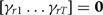; the score test evaluates the gradient and second derivative at the null of the log-likelihood with respect to this parameter vector. As the test is evaluated at the null, there is no need to fit the extended model. For each realization of the complete data by the MCMC sampler, we evaluate the score vector U as a vector whose t-th element is and the information matrix V as a matrix with element equal to . The score is evaluated as the posterior mean of U, and the observed information as the complete information (posterior mean of V) minus the missing information (posterior covariance of U).³¹ This yields a summary chi-square test with T – 1 degrees of freedom.

Data set

The population sample is from the ORCADES study of individuals originating in the Orkney Islands, Scotland, UK.²⁰ A total of 1017 healthy adults (mean age 53 years; range 16–100 years; 60% female) were examined in 2005–07 and over 100 quantitative traits were measured, including fasting plasma glucose, lipid profile and uric acid levels. Detailed pedigree information was collected from which to calculate the relationship matrix. Metabolic syndrome was defined as the presence of at least three of the Adult Treatment Panel III criteria:³² waist girth >102 cm in men or >88 cm in women, systolic blood pressure ≥130 mmHg or anti-hypertensive medication, plasma glucose (>6.1 mmol/l), plasma high-density lipoprotein cholesterol (mmol/l) (<1.03 in men or <1.29 in women), plasma triglyceride ≥1.70 mmol/l. The prevalence of metabolic syndrome by these criteria was 20%. In a random subset of 706 individuals, six SNPs in the urate transporter gene SLC2A9 were typed using a TaqMan assay.

Computational methods

Plasma urate levels were scaled before analysis to have standard deviation (SD) of 1. To allow for intra-individual variation in measured urate levels, the model was specified with intra-individual variance of 0.2. This is equivalent to the intra-class correlation of 0.80 that has been reported for urate measured on two occasions.³³ The kinship matrix A for the ORCADES participants was calculated from the pedigree using the R package kinship (http://cran.r-project.org/web/packages/kinship/kinship.pdf. The JAGS program (http://www-fis.iarc.fr/martyn/software/jags) was used to sample the posterior density. Models were specified with a flat prior on the allele frequency, diffuse Gaussian priors (mean zero, variance 1000) on regression coefficient, and a diffuse gamma prior (shape 0.01, inverse scale 0.01) on the precision parameter in the linear regression of urate on genotype. Age and sex were included as covariates in both the regression models. With the current version of JAGS, it is not computationally feasible to model polygenic effects as predictors in a logistic regression model, as this gives rise to a non-conjugate full conditional distribution for the polygenic effects. To model polygenic effects, a probit regression model was therefore substituted for the logistic regression model. Probit regression is similar to logistic regression, but gives more weight to outliers because the probit distribution is less heavy-tailed than the logistic distribution.³⁴ For the probit regression model, the Gaussian errors were specified with a prior mean of zero and variance of 1; the value specified for the variance affects the scaling of the regression parameters but not the parameter θ. All 1017 participants were included in the model: missing values for genotype, urate level and outcome were sampled from their joint posterior distribution. For each model, two sampling chains were run with a burn-in of 1000 iterations followed by 20 000 iterations for inference. The R package coda was used to assess convergence by Geweke diagnostics and mixing of the two chains by Gelman–Rubin diagnostics. The number of iterations was set so as to obtain stable estimates of the lod score. The R function density was used with Gaussian kernel to compute the marginal density from posterior samples.

Results

The SNPHAP program was able to assign haplotypes with >90% posterior probability in 674 of the 706 individuals who were genotyped at least one locus. The three commonest six-locus haplotypes accounted for 90% of estimated haplotype frequencies, As the associations of urate with haplotype were slightly weaker than the associations with individual SNPs, the effects of genotype on plasma urate were modelled as effects of unphased genotypes. Of the six SNPs typed, rs13129697 showed the strongest univariate association with urate levels in classical linear regression analyses fitted by maximum likelihood. The frequency of the rs13129697 allele associated with higher urate levels was 0.24. The slope of the logistic regression of metabolic syndrome on urate was 0.79 per SD (), and the slope of the linear regression of urate on rs13129697 genotype (coded as 0, 1, 2 copies) was 0.22 odds ratio (OR) 1.25, . The slope of the logistic regression of metabolic syndrome on genotype was −0.27 (OR 0.76, ). This compares with a predicted slope of +0.17 (0.22 × 0.79) if the association of urate with metabolic syndrome were causal. An approximate estimator of the causal effect parameter can be obtained as .

All six SNPs in SLC2A9 were included as predictors in the Bayesian model linear regression model for urate. Table 1 shows the posterior means and 95% credible intervals in a model specified with diffuse priors on all parameters including the effect ratio parameter θ. The posterior mean for the causal effect parameter β_x was −1.25 (95% credible interval −2.91 to 0.05). The posterior mean for the confounding effect parameter β was 2.63 (95% credible interval 1.24–4.38). The posterior means and credible intervals were similar when an alternative parameterization for causal and confounding effects was used, although mixing was slower.

Table 1.

Posterior means and 95% credible intervals for parameters in a model with diffuse priors

Parameter	Posterior mean	Percentile 2.5	Percentile 97.5
Linear regression: effect of genotype on urate
rs737267	0.16	−0.04	0.37
rs13129697	0.26	0.10	0.42
rs1014290	0.05	−0.15	0.25
rs6449213	0.04	−0.20	0.26
rs13131257	−0.12	−0.32	0.08
rs4447863	0.07	−0.02	0.15
Residual precision (inverse variance) of urate	2.09	1.83	2.38
Logistic regresssion: effect of urate on metabolic syndrome
Causal effect parameter βx	−1.25	−2.91	0.05
Confounding effect parameter βe	2.63	1.24	4.38
Causal/crude effect ratio parameter θ	−0.91	−2.20	0.04

The log-likelihood function for the causal/crude effect ratio parameter θ, scaled to have zero value at θ = 0, is shown in Figure 3. In a model that ignores intra-individual variability in plasma urate levels, the lod score favouring θ = 0 (association attributable entirely to confounding) over θ = 1 (association attributable entirely to causal effect) is 1.38: equivalent to a likelihood ratio of 24 : 1. When intra-individual variability in plasma urate is allowed for in the model by setting the intra-class correlation to 0.8, the evidence against a causal explanation for the crude association of urate with metabolic syndrome is stronger (lod score 2.34). The data give most support to negative values of θ, equivalent to a causal effect of urate that is in the opposite direction to the crude (observed) association with metabolic syndrome. A score test for residual association of genotype with outcome yielded no evidence against the no-pleiotropy assumption (χ² 4.4 with 5 df).

Figure 3.

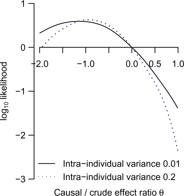
Log-likelihood of causal/crude effect ratio θ, scaled to zero at θ = 0: comparisons of models ignoring and allowing for intra-individual variability in urate levels

Figure 4 compares probit regression models with and without allowing for relatedness through inclusion of additive polygenic effects on urate levels and metabolic syndrome in the model. Allowing for relatedness yields a flatter log-likelihood function but has little effect on the lod score for a non-causal versus a causal explanation.

Figure 4.

Log-likelihood of causal/crude effect ratio θ, scaled to zero at θ = 0: comparison of models ignoring and allowing for relatedness

Discussion

The Bayesian formulation helps to make explicit the assumptions underlying instrumental variable analysis, and to distinguish assumptions that are fundamental to the approach from those that are required to calculate estimators. For instance, we are free (except where we have to model polygenic effects in related individuals) to specify logistic regression models for effects on a binary intermediate variable, rather than probit regression models that are more restrictive than the information available in the data. Other linear models, such as Cox regression for survival data, are straightforward to fit with this approach.

With a binary intermediate variable, we would have to specify the unobserved confounder as a latent variable, because its effect on the intermediate variable cannot be marginalized out analytically, as it can when the intermediate variable is modelled as a Gaussian node. We are not restricted to generalized linear models; thus Bayesian instrumental variable analysis can be extended to encompass non-linear confounding effects, using a Dirichlet process mixture to model the covariance of residuals in the intermediate phenotype and the outcome.¹⁹ We do not have to assume a monotonic effect of the instrument on the intermediate phenotype; where the instrument is a randomization procedure, we could fit a model that allows some individuals to ‘defy’ the instrument.¹⁸ The flexibility of programs such as JAGS makes it straightforward to allow for intra-individual variability in the intermediate phenotype by modelling its underlying (stable) value as a latent variable. We would expect that failure to allow for intra-individual variation in the intermediate phenotype would lead to underestimation of the crude effect but not the causal effect of the intermediate phenotype on the outcome. Our results are consistent with this: in comparison with a model that allows for intra-individual variation, a model that ignores intra-individual variation yields a likelihood peak for the ratio θ of causal to crude effect that is further from zero.

The fully Bayesian approach to hypothesis testing eliminates the difficulties of constructing ‘estimators’ because nothing is estimated: hypothesis tests are obtained directly from the likelihood, with nuisance parameters integrated out. If parameter estimates are required, they can be obtained from the posterior distribution as posterior means and credible intervals, as demonstrated in this article. Such Bayesian estimates usually have excellent sampling properties over repeated experiments.¹¹ As Bayesian inference does not rely on asymptotic arguments, the problems of inference with ‘weak’ instruments discussed by others⁹ do not arise: if the instrument is too weak, the log-likelihood function will be nearly flat, implying that the study has yielded very little information. The posterior density, however, will be dominated by the prior when the instrument is weak. As Kleibergen and Zivot have demonstrated,¹⁷ some classical instrumental variable methods can be viewed as limiting cases of Bayesian methods with inappropriate priors. Thus we have shown above that the classical ‘methods of moments estimator’ for the causal effect parameter is a limiting case of a Bayesian estimate in which priors on the effects of the instrument on the biomarker and the outcome are (inappropriately) specified to be independent.

In large samples where regularity assumptions hold, the log-likelihood function is approximately quadratic, as is the log-likelihood of the effect ratio parameter θ in this data set. In this situation, classical significance tests and interval estimates can be obtained from the likelihood function: for instance, a test of the null hypothesis of equality of causal and crude effects can be obtained from the difference between the peak log-likelihood and the log-likelihood at θ = 1. Even where asymptotic properties of the log-likelihood do not hold, inference based on the likelihood ratio is still valid. Construction of ‘estimators’ that are not based on the likelihood is of uncertain value: even if such estimators have correct sampling properties, they violate the likelihood principle (the principle that the log-likelihood of a parameter contains conveys all information in the data about that parameter³⁵).

There has been controversy over whether causal relationships can be represented by probabilistic graphical models without invoking ‘counterfactual’ arguments.^6,36,37 The likelihood principle³⁵ implies that counterfactual arguments can therefore contribute to inference of causation from data only to the extent that they specify the likelihoods of causal and non-causal models, given the data.

We now discuss in more detail the three fundamental assumptions of the instrumental variable argument as applied to genetic instruments: no confounding of the effect of genotype on outcome, no pleiotropy (equivalent to the ‘exclusion restriction’ of classical instrumental variable analysis¹⁸), and that effects of different settings of the intermediate phenotype are independent of the instrument (no developmental compensation). With genetic instruments, we can assume no confounding not only for the effect of genotype on outcome but also for the effect of genotype on intermediate trait: this strengthens the basis for combining results from different studies, as outlined below. The laws of Mendelian genetics guarantee that genetic associations are unconfounded (other than by alleles at linked loci) if population stratification has been controlled in the design or analysis. Inference of population stratification is now straightforward, using either principal components analysis with a genome-wide panel of tag SNPs³⁸ or modelling admixture with a subset of ancestry-informative markers.³¹ Recent experience with genome-wide association studies has shown that these methods are adequate to control for confounding by population stratification, even when the genetic associations under study are weak.

The assumption of no pleiotropy—that the effect of genotype on outcome is mediated only through the intermediate trait—relies mainly on biological plausibility: for instance, understanding the role of nicotine in maintaining smoking behaviour (and the lack of a known role of nicotine in carcinogenesis) makes it plausible that any effect of nicotine receptor genotype on lung cancer risk is mediated through effects on smoking.³⁹ One situation in which the assumption of no pleiotropy is likely to be violated is where the intermediate trait is measured as the level of the gene product, and there is a non-synonymous variant (one that alters protein sequence) in the gene used as instrument. An effect on disease mediated through altered protein sequence would not necessarily be captured by measurement of the level of the protein. This can be dealt with by typing the non-synonymous variant and including it in the model as a covariate, rather than as an instrumental variable. Where multiple loci have been typed in the gene used as instrument, we can test the assumption of no pleiotropy by testing for residual association of genotype with the outcome (conditional on the expected value of the intermediate trait given multilocus genotype) as demonstrated here. If the assumption of no confounding of genotypic effects holds, this is a specific test for pleiotropy. This is similar to the argument used to construct tests of ‘overidentifying restrictions’ in classical instrumental variable analysis.⁴⁰ In a Bayesian framework, it is straightforward to construct such tests by averaging over the posterior distribution to compute the score vector and information matrix. As most genetic association studies now type multiple SNPs in each gene, this test has wide application.

The assumption of no developmental compensation usually relies upon understanding biological pathways. In principle, it could be tested by measuring possible compensatory effects. This is a rather stronger assumption than is typically made for instrumental variable problems, where it is customary to emphasize that the results may depend upon the instruments used.

For the instrumental variable argument to be valid, it is not necessary that all three effects—genotype on intermediate phenotype, genotype on outcome and intermediate phenotype on outcome—are inferred from a single study. Inference of these effects from different studies does not change the modelling approach described here, as Bayesian modelling automatically uses all available data to infer the model parameters. Because associations with genotype are unconfounded, it is reasonable to assume that the effects of genotype on intermediate variable and outcome will not differ between study populations of similar genetic background unless factors that modify the effect of genotype differ markedly between the study populations, The association of intermediate phenotype with outcome may vary between study populations because of confounding, but the instrumental variable analysis should be able to deal with this. The ability to combine information from different studies is important because the most efficient study designs for inferring the effect of genotype on outcome are not usually optimal for inferring the mediating effect of the intermediate variable on outcome. Usually, the effect of the intermediate variable on a disease outcome is examined in a cohort study, so that measurements of the intermediate variable can be obtained before disease onset. For inferring the effects of genotype on disease outcome, however, case–control studies are the most efficient design,⁴¹ and cohort studies of adequate size to detect small effects of genotype on outcome are usually unfeasible. In Appendix 1, we show that for typical assumptions about allele frequency, size of genetic effect on the intermediate variable, Type 1 error rate and Type 2 error rate, the number of cases required in a genetic case–control study with equal numbers of cases and controls is of the order of 100 times larger than the number of cases required to detect the association of the biomarker with outcome in a cohort study. Thus, for instance, where the standardized OR for the effect of a biomarker on disease risk is 1.5 (typical of metabolic risk factors for cardiovascular disease), only 63 cases at follow-up are required for 90% power to detect this association at P < 0.05 in a case–control study, but (assuming allele frequency of 0.2 and standardized effect size of 0.25 for the effect of genotype on the biomarker, about 6000 cases and 6000 controls are required to detect the predicted genotype–disease association. This disparity in sample size requirements means that it is not usually feasible to infer the intermediate variable–outcome and genotype–outcome associations in a single study as in the classical ‘instrumental variable’ approach.

The emphasis of this article is on statistical methods for instrumental variable analysis, rather than on the association of urate levels with metabolic syndrome⁴² that we have used to demonstrate the application of these methods. If the assumption of no pleiotropy—that any effect of SLC2A9 on the metabolic syndrome is mediated only through urate levels—is correct, our results suggest that the association is unlikely to be causal, and that raised urate levels may even protect against metabolic syndrome. There is some indirect support for this from clinical studies showing that administration of uric acid has effects which are possibly beneficial, such as reversal of endothelial dysfunction and increase of anti-oxidant capacity.^43,44 However, as SLC2A9 is also a fructose transporter,²⁰ the assumption of no pleiotropy is open to question. Although the score test does not yield any evidence of pleiotropy, this test would be more convincing if it could be demonstrated that the SNPs or haplotypes influencing fructose transport differed from those influencing urate transport.

Instrumental variable analysis with genetic instruments has been applied mainly to quantitative biomarkers of disease identified in cross-sectional or prospective studies, though in principle it can be applied to any trait or exposure for which a suitable genetic instrument is available: for instance, nicotine receptor genotype may be a suitable instrumental variable for exposure to tobacco smoke. As more loci that influence intermediate traits are discovered through scoring of genome-wide SNP panels in large collections of individuals on whom multiple quantitative traits have been measured, there will be many more opportunities for using instrumental variable analyses to distinguish between causal and non-causal biomarkers of disease risk. The methods described here have application to instrumental variable modelling of other problems, such as allowing for non-compliance in randomized trials (where assignment can be considered as the instrumental variable and treatment received as the intermediate phenotype⁵) or estimating the effect of emergency therapeutic intervention using proximity to hospital as instrumental variable.⁴⁵ In these contexts, a key advantage of Bayesian computationally intensive methods may be the ability to handle latent variables and missing data.

Implementation of these methods depends upon the availability of software for Bayesian modelling. The two main general purpose programs for MCMC sampling in graphical models are BUGS and JAGS. JAGS uses the same model description language as BUGS, but is fully portable across platforms as it is written in C++. The current version of JAGS has several limitations for type of analysis described here: mixing of the sampler for regression parameters is slow, and it is not computationally feasible to include polygenic effects in a logistic regression model because the full conditional distribution for the polygenic effects is non-conjugate. These limitations can be overcome by implementing a more efficient joint sampler for regression model parameters, and by reparameterizing the logistic regression model as a scale mixture of probit regression models so as to allow conjugate updating of random effects.⁴⁶ Work is in progress to implement these extensions in JAGS. A more challenging problem is to extend this approach to more complex problems with multiple genes and biomarkers, where inference of causal relationships requires searching a large space of possible models. Such model choice problems are not, except in special cases, tractable to MCMC simulation but may be tractable to approximate inference methods such as variational Bayes and expectation-propagation.⁴⁷

URLs

JAGS scripts for the model described here: http://homepages.ed.ac.uk/pmckeigu/mendelrand JAGS program: http://www-fis.iarc.fr/~martyn/software/jags

Funding

UK Medical Research Council (grant G0800604 to P.M.M.); The ORCADES study was supported by a Royal Society fellowship (to J.F.W.), by the Chief Scientist Office of the Scottish Government Health Directorates and by the facilities of the Wellcome Trust Clinical Research Facility, Edinburgh.

Conflict of interest: None declared.

KEY MESSAGES.

• Using genotype as an ‘instrument’ it is possible in principle to distinguish between causal and non-causal explanations of a biomarker–disease association, but classical methods for instrumental variable analysis have limitations.

• Bayesian computationally instensive methods overcome these limitations, and can evaluate the weight of evidence favouring a causal explanation over confounding.

• A Bayesian analysis using the urate transporter gene SLC2A9 as instrument yields a likelihood ratio of 218 : 1 favouring confounding over causation as explanation of the association of plasma urate levels with metabolic syndrome.

• Where multiple SNPs in a gene have been typed, it is possible to test a key assumption of the instrumental variable method that effects of the instrument on the outcome are mediated only through the biomarker.

• Applying this approach in practice will typically require combining information from cross-sectional or cohort studies and with information from large genetic case–control studies.

Appendix 1: sample size requirements for instrumental variable analysis with genetic instruments

For given Type 1 and Type 2 error probabilities and study design, the sample size required to detect an effect of size d is proportional to 1/d²V, where V is the Fisher information (expectation of minus the second derivative of the log-likelihood of the effect size) from a single observation. For a single observation from a logistic regression model (in which the effect is measured as the log OR), the Fisher information is ϕ(1−ϕ)v, where ϕ is the probability of being a case, and v is the variance of the predictor variable.

For a cohort design testing for association of a rare disease (ϕ close to 0) with a quantitative trait that is scaled to have variance of 1, the Fisher information is simply the total number n of cases yielded by the cohort study. For a case–control design with N cases and N controls (ϕ = 0.5), testing for an effect on disease risk of genotype (coded as 0, 1, 2) at an SNP with allele frequency p, the Fisher information is . For allele frequency 0.2, this evaluates to N/6.25. Thus, in this situation the number N of cases required for a case–control study to detect the effect (measured as log OR associated with one extra copy of the disease-associated allele) is 6.25 times larger than the number n of cases required for a cohort study to detect an effect of the same size (measured as log OR associated with change of 1 SD) of a continuous trait on disease risk.

In reality, the size of the genotypic effect α_g on the intermediate phenotype is usually modest: typically no more than 0.25 SD for each extra copy of the trait-raising allele. As sample size scales inversely with the square of the effect size, this implies that the case–control collection would have to be 100 (16 × 6.25) times larger (in terms of number of cases) than the cohort study for the effect of genotype on disease to be detected in a conventional significance test. For a Bayesian hypothesis test, the sample size requirements for the case–control study of genotype–disease association are similar. Bayesian sample size requirements for an experiment comparing two hypotheses can be calculated by specifying the expected log-likelihood ratio (ELOD) favouring the true hypothesis over the alternative. For a given effect size d, the sample size required for 90% power to detect this effect at 5% significance in a classical hypothesis test is (Z_0.9 + Z_0.975)²/(d²V) = 10.5/(d²V), and the sample size required for an ELOD of log(100) favouring this effect size over the null is .

References

- 1.Smith GD, Ebrahim S. What can Mendelian randomisation tell us about modifiable behavioural and environmental exposures? Br Med J. 2005;330:1076–79. doi: 10.1136/bmj.330.7499.1076. [DOI] [PMC free article] [PubMed] [Google Scholar]
- 2.Keavney B, Danesh J, Parish S, et al. Fibrinogen and coronary heart disease: Fibrinogen and coronary heart disease: test of causality by ‘Mendelian randomization’. Int J Epidemiol. 2006;35:935–43. doi: 10.1093/ije/dyl114. [DOI] [PubMed] [Google Scholar]
- 3.Thomas DC, Conti DV. Commentary: the concept of 'Mendelian Randomization'. Int J Epidemiol. 2004;33:21–25. doi: 10.1093/ije/dyh048. [DOI] [PubMed] [Google Scholar]
- 4.Newhouse JP, McClellan M. Econometrics in outcomes research: the use of instrumental variables. Annu Rev Public Health. 1998;19:17–34. doi: 10.1146/annurev.publhealth.19.1.17. [DOI] [PubMed] [Google Scholar]
- 5.Greenland S. An introduction to instrumental variables for epidemiologists. Int J Epidemiol. 2000;29:722–29. doi: 10.1093/ije/29.4.722. [DOI] [PubMed] [Google Scholar]
- 6.Hernán MA, Robins JM. Instruments for causal inference: an epidemiologist's dream? Epidemiology. 2006;17:360–72. doi: 10.1097/01.ede.0000222409.00878.37. [DOI] [PubMed] [Google Scholar]
- 7.Wehby GL, Ohsfeldt RL, Murray JC. ‘Mendelian randomization’ equals instrumental variable analysis with genetic instruments. Stat Med. 2008;27:2745–49. doi: 10.1002/sim.3255. [DOI] [PMC free article] [PubMed] [Google Scholar]
- 8.Timpson NJ, Lawlor DA, Harbord RM, et al. C-reactive protein and its role in C-reactive protein and its role in metabolic syndrome: Mendelian randomisation study. Lancet. 2005;366:1954–59. doi: 10.1016/S0140-6736(05)67786-0. [DOI] [PubMed] [Google Scholar]
- 9.Lawlor DA, Harbord RM, Sterne JAC, Timpson N, Smith GD. Mendelian randomization: using genes as instruments for making causal inferences in epidemiology. Stat Med. 2008;27:1133–328. doi: 10.1002/sim.3034. [DOI] [PubMed] [Google Scholar]
- 10.Chernozhukov V, Hansen C. The reduced form: a simple approach to inference with weak estimators. Econ Lett. 2008;100:68–71. [Google Scholar]
- 11.Jaynes ET. Confidence intervals vs Bayesian intervals. In: Harper WL, Hooker CA, editors. Foundations of Probability Theory, Statistical Inference and Statistical Theories of Science. Vol. II. Dordrecht: Reidel; 1976. pp. 175–257. [Google Scholar]
- 12.Zech G. Frequentist and Bayesian confidence intervals. Eur Phy J. 2002;12:1–81. [Google Scholar]
- 13.Rassen JA, Schneeweiss S, Glynn RJ, Mittleman MA, Brookhart MA. Instrumental variable analysis for estimation of treatment effects with dichotomous outcomes. Am J Epidemiol. 2009;169:273–84. doi: 10.1093/aje/kwn299. [DOI] [PubMed] [Google Scholar]
- 14.Vansteelandt S, Goetghebeur E. Causal inference with generalized structural mean models. J Roy Stat Soc B. 2003;65:817–35. [Google Scholar]
- 15.Robins J, Rotnitzky A. Estimation of treatment effects in randomised trials with noncompliance and a dichotomous outcome using structural mean models. Biometrika. 2004;91:763–83. [Google Scholar]
- 16.Thompson JR, Minelli C, Abrams KR, Tobin MD, Riley RD. Mendelian Meta-analysis of genetic studies using Mendelian randomization–a multivariate approach. Stat Med. 2005;24:2241–54. doi: 10.1002/sim.2100. [DOI] [PubMed] [Google Scholar]
- 17.Kleibergen F, Zivot E. Bayesian and classical approaches to instrumental variable regression. J Econ. 2003;114:29–72. [Google Scholar]
- 18.Imbens GW, Rubin DB. Bayesian inference for causal effects in randomized experiments with noncompliance. Ann Stat. 1997;25:305–27. [Google Scholar]
- 19.Conley TG, Hansen CB, McCulloch RE, Rossi PE. A semi-parametric Bayesian approach to the instrumental variable problem. J Econ. 2008;138:63–103. [Google Scholar]
- 20.Vitart V, Rudan I, Hayward C, et al. SLC2A9 is a newly identified urate SLC2A9 is a newly identified urate transporter influencing serum urate concentration, urate excretion and gout. Nat Genet. 2008;40:437–42. doi: 10.1038/ng.106. [DOI] [PubMed] [Google Scholar]
- 21.Wallace C, Newhouse SJ, Braund P, et al. Genome-wide association study identifies genes for biomarkers of cardiovascular disease: serum urate and dyslipidemia. Am J Hum Genet. 2008;82:139–49. doi: 10.1016/j.ajhg.2007.11.001. [DOI] [PMC free article] [PubMed] [Google Scholar]
- 22.Blower DJ. An easy derivation of logistic regression from the Bayesian and maximum entropy perspective. In: Erickson GJ, Zhai Y, editors. 23rd International Workshop on Bayesian Inference and Maximum EntropyMethods in Science and Engineering. Vol. 707. Melville, NY: American Institute of Physics; 2004. pp. 30–43. [Google Scholar]
- 23.Jaynes ET. Probability Theory: The Logic of Science. Cambridge, UK: Cambridge University Press; 2003. [Google Scholar]
- 24.Andrews DF, Mallows CL. Scale mixtures of normal distributions. J Roy Stat Soc. 1974;B36:99–102. [Google Scholar]
- 25.Arellano M. Sargans instrumental variables estimation and the generalized method of moments. J Bus Econ Stat. 2002;20:450–59. [Google Scholar]
- 26.Palmer TM, Thompson JR, Tobin MD, Sheehan NA, Burton PR. Adjusting for bias and unmeasured confounding in Mendelian randomization studies with binary responses. Int J Epidemiol. 2008;37:1161–68. doi: 10.1093/ije/dyn080. [DOI] [PubMed] [Google Scholar]
- 27.Fisher RA. The correlation between relatives on the supposition of Mendelian inheritance. Philos Trans R Soc Edin. 1918;52:399–433. [Google Scholar]
- 28.Morton NE, MacLean CJ. Analysis of family resemblance. 3. Complex segregation of quantitative traits. Am J Hum Genet. 1974;26:489–503. [PMC free article] [PubMed] [Google Scholar]
- 29.Aulchenko YS, de Koning DJ, Haley C. Genomewide rapid association using mixed model and regression: a fast and simple method for genomewide pedigree-based quantitative trait loci association analysis. Genetics. 2007;177:577–85. doi: 10.1534/genetics.107.075614. [DOI] [PMC free article] [PubMed] [Google Scholar]
- 30.MacKay DJC. Information Theory, Inference and Learning Algorithms. Cambridge, UK: Cambridge University Press; 2003. [Google Scholar]
- 31.Hoggart CJ, Parra EJ, Shriver MD, et al. Control of confounding of genetic associations in stratified populations. Am J Hum Genet. 2003;72:1492–504. doi: 10.1086/375613. [DOI] [PMC free article] [PubMed] [Google Scholar]
- 32.Grundy SM, Brewer HB, Cleeman JI, Smith SC, Lenfant C. Definition of metabolic syndrome: Report of the National Heart, Lung, and Blood Institute/American Heart Association conference on scientific issues related to definition. Circulation. 2004;109:433–38. doi: 10.1161/01.CIR.0000111245.75752.C6. [DOI] [PubMed] [Google Scholar]
- 33.Whitfield JB, Martin NG. Inheritance and alcohol as factors influencing plasma uric acid levels. Acta Genet Med Gemellol. 1983;32:117–26. doi: 10.1017/s0001566000006401. [DOI] [PubMed] [Google Scholar]
- 34.Congdon P. Applied Bayesian Modelling. Hoboken, NJ: Wiley; 2003. [Google Scholar]
- 35.Birnbaum A. On the foundations of statistical inference. J Am Stat Assoc. 1962;57:269–326. [Google Scholar]
- 36.Dawid AP. Counterfactuals: help or hindrance? Int J Epidemiol. 2002;31:429–30. [PubMed] [Google Scholar]
- 37.Hfler M. Causal inference based on counterfactuals. BMC Med Res Methodol. 2005;5:28. doi: 10.1186/1471-2288-5-28. [DOI] [PMC free article] [PubMed] [Google Scholar]
- 38.Patterson N, Price AL, Reich D. Population structure and eigenanalysis. PLoS Genet. 2006;2:e190. doi: 10.1371/journal.pgen.0020190. [DOI] [PMC free article] [PubMed] [Google Scholar]
- 39.Thorgeirsson TE, Geller F, Sulem P, et al. A variant associated with nicotine dependence, lung cancer and peripheral arterial disease. Nature. 2008;452:638–42. doi: 10.1038/nature06846. [DOI] [PMC free article] [PubMed] [Google Scholar]
- 40.Sargan JD. The estimation of economic relationships using instrumental variables. Econometrica. 1958;26:393–415. [Google Scholar]
- 41.Clayton D, McKeigue PM. Epidemiological methods for studying genes and environmental factors in complex diseases. Lancet. 2001;358:1356–60. doi: 10.1016/S0140-6736(01)06418-2. [DOI] [PubMed] [Google Scholar]
- 42.Feig DI, Kang DH, Johnson RJ. Uric acid and cardiovascular risk. N Engl J Med. 2008;359:1811–21. doi: 10.1056/NEJMra0800885. [DOI] [PMC free article] [PubMed] [Google Scholar]
- 43.Waring WS, Convery A, Mishra V, Shenkin A, Webb DJ, Maxwell SRJ. Uric acid reduces exercise-induced oxidative stress in healthy adults. Clin Sci. 2003;105:425–30. doi: 10.1042/CS20030149. [DOI] [PubMed] [Google Scholar]
- 44.Waring WS, McKnight JA, Webb DJ, Maxwell SRJ. Uric acid restores endothelial function in patients with type 1 diabetes and regular smokers. Diabetes. 2006;55:3127–32. doi: 10.2337/db06-0283. [DOI] [PubMed] [Google Scholar]
- 45.McClellan M, McNeil BJ, Newhouse JP. Does more intensive treatment of acute myocardial infarction in the elderly reduce mortality? Analysis using instrumental variables. JAMA. 1994;272:859–66. [PubMed] [Google Scholar]
- 46.Holmes CC, Held L. Bayesian auxiliary variable methods for binary and multinomial regression. Bayesian Anal. 2004;1:145–68. [Google Scholar]
- 47.Beal MJ, Ghahramani Z. Variational Bayesian learning of directed graphical models with hidden variables. Bayesian Anal. 2006;1:793–832. [Google Scholar]