Estimating Optimal Dynamic Regimes: Correcting Bias under the Null

Abstract

A dynamic regime provides a sequence of treatments that are tailored to patient-specific characteristics and outcomes. In 2004 James Robins proposed g-estimation using structural nested mean models for making inference about the optimal dynamic regime in a multi-interval trial. The method provides clear advantages over traditional parametric approaches. Robins’ g-estimation method always yields consistent estimators, but these can be asymptotically biased under a given structural nested mean model for certain longitudinal distributions of the treatments and covariates, termed exceptional laws. In fact, under the null hypothesis of no treatment effect, every distribution constitutes an exceptional law under structural nested mean models which allow for interaction of current treatment with past treatments or covariates. This paper provides an explanation of exceptional laws and describes a new approach to g-estimation which we call Zeroing Instead of Plugging In (ZIPI). ZIPI provides nearly identical estimators to recursive g-estimators at non-exceptional laws while providing substantial reduction in the bias at an exceptional law when decision rule parameters are not shared across intervals.

1 Introduction

In a study aimed at estimating the mean effect of a treatment on a time-dependent outcome, dynamic treatment regimes are an obvious choice to consider. A dynamic regime is a function that takes treatment and covariate history as arguments; the value returned by the function is the treatment to be given at the current time. A dynamic regime provides a sequence of treatments that are tailored to patient-specific characteristics and outcomes. A recently proposed method of inference (Robins, 2004) is g-estimation using structural nested mean models: this method is semi-parametric and is robust to certain types of mis-specification and in this regard it is superior to traditional parametric approaches. However, g-estimation of certain structural nested mean models is asymptotically biased under specific data distributions which Robins has termed the exceptional laws. At exceptional laws, g-estimators of parameters for optimal structural nested mean models are asymptotically biased and exhibit non-regular behaviour.

The aim of this paper is to provide a means of reducing the asymptotic bias of g-estimators in the presence of exceptional laws. Exceptional laws are discussed in the optimal dynamic regimes literature only by Robins, (2004); there, a method of detecting these laws and improving coverage of confidence intervals, but not the bias of point estimates, is proposed.

Structural nested mean models and g-estimation are discussed in section 2.1, followed by a detailed explanation of exceptional laws in g-estimation in section 2.2. Section 3.2 describes a method of reducing the asymptotic bias due to exceptional laws which we call Zeroing Instead of Plugging In (ZIPI), with theoretical properties derived in section 3.3. Sections 3.4 and 3.5 compare ZIPI to g-estimation and to the Iterative Minimization for Optimal Regimes (IMOR) method proposed by Murphy (2003). Section 4 concludes.

2 Inference via g-estimation and exceptional laws

2.1 Inference for optimal dynamic regimes: structural nested mean models and g-estimation

We consider the estimation of treatment effect in a longitudinal study. All of the methods discussed in this paper may be extended to a finite number of treatment intervals. We focus on the two-interval case where a single covariate is used to determine the optimal rule at each interval.

Notation

Notation is adapted from Murphy (2003) and Robins (2004). Treatments are taken at K fixed times, t₁,…,t_K. L_j are the covariates measured prior to treatment at the beginning of the j^th interval, while A_j is the treatment taken subsequent to having measured L_j. Y is the outcome observed at the end of interval K; larger values of Y are favorable. Random variables are upper case; specific values, or fixed functions are lower-case. Denote a variable X_j at t_j and its history, (X₁, X₂,…,X_j), by X̄_j. Finally, denote a treatment decision at t_j that depends on history, L̄_j, Ā_j−1, by D_j ≡ d_j(L̄_j, Ā_j−1).

In the two-interval case, treatments are taken at two fixed times, t₁ and t₂, with outcome measured at t₃. The covariates measured prior to treatment at the beginning of the first and second intervals, i.e. at t₁ and t₂, are L₁ and L₂, respectively. In particular, L₁ represents baseline covariates and L₂ includes time-varying covariates which may depend on treatment received at t₁. The treatment given subsequent to observing L_j is A_j, j = 1, 2. Response Y is measured at t₃. Thus, the data are, chronologically, (L₁, A₁, L₂, A₂, Y).

Throughout this paper, models are explained in terms of potential outcomes: the value of a covariate or the outcome that would result if a subject were assigned to a treatment possibly different from the one that they actually received. In the two-interval case we denote by L₂(a₁) a subject’s potential covariate at the beginning of the second interval if treatment a₁ is taken by that subject, and Y(a₁, a₂) denotes the potential end-of-study outcome if regime (a₁, a₂) is followed.

Potential outcomes adhere to the axiom of consistency: L₂(a₁) ≡ L₂ whenever treatment a₁ is actually received and Y(a₁, a₂) ≡ Y whenever (a₁, a₂) is received. That is, the actual and counterfactual covariates (or outcome) are equal when the potential regime is the regime actually received.

We use the following definitions: an estimator ψ̂_n of the parameter ψ^† is $\sqrt{n}$-consistent if $\sqrt{n}({\hat{\psi }}_n-{\psi }^{†})=O_p(1)$ with respect to any distribution P in the model. Similarly, if under P, $\sqrt{n}({\hat{\psi }}_n-{\psi }^{†})\stackrel{D}{\to }T$, and E|T| < ∞ then E(T) is the $(\sqrt{n})$ asymptotic bias of ψ̂_n under P, which we denote AsyBiasp(ψ̂_n). If for some law P in the model, AsyBiasp(ψ̂_n) = 0, then ψ̂_n is said to be $(\sqrt{n})$ asymptotically unbiased under P. (We will usually suppress the $\sqrt{n}$ and the P in our notation.) As shall be seen, g-estimators are $\sqrt{n}$-consistent under all laws, however they are not asymptotically unbiased under certain distributions of the data, which, following Robins (2004), we term ‘exceptional laws’ (see section 2.2).

Assumptions

To estimate the effect of a dynamic regime, we require the stable unit treatment value assumption (Rubin, 1978), which states that a subject’s outcome is not influenced by other subjects’ treatment allocation. In addition we assume that there are no unmeasured confounders (Robins, 1997), i.e. for any regime ā_K,

$$A_j╨(L_{j+1}({\mathit{ā}}_j),\dots ,L_K({\mathit{ā}}_{K-1}),Y({\mathit{ā}}_K))|{\overline{L}}_j,{\mathit{Ā}}_{j-1}={\mathit{ā}}_{j-1}.$$

In a trial in which sequential randomization is carried out, the latter assumption always holds. In two intervals for any a₁, a₂ we have that A₁ ╨ (L₂(a₁), Y(a₁, a₂)) | L₁ and A₂ ╨ Y(a₁, a₂) | (L₁, A₁ = a₁, L₂), that is, conditional on history, treatment received in any interval is independent of any future potential outcome.

Without further assumptions, the optimal regime may only be estimated from among the set of feasible regimes (Robins, 1994), i.e. those treatment regimes that have positive probability; in order to make non-parametric inference about a regime we require some subjects to have followed it.

Structural nested mean models and g-estimation

Robins (2004, p. 209–214) produced a number of estimating equations for finding optimal regimes using structural nested mean models (SNMM) (Robins, 1994). We use a subclass of SNMMs called the optimal blip-to-zero functions, denoted by γ_j(l̄_j, ā_j), defined as the expected difference in outcome when using the “zero” regime instead of treatment a_j at t_j, in subjects with treatment and covariate history l̄_j, ā_j−1 who subsequently receive the optimal regime. The “zero” regime, which we denote 0_j, can be thought of as placebo or standard care; the optimal strategy at time j is denoted $d_j^{\mathit{\text{opt}}}({\overline{l}}_j,{\mathit{ā}}_{j-1})$. The optimal treatment regime subsequent to being prescribed a_j (or 0_j) at t_j may depend on prior treatment and covariate history i.e. what is optimal subsequent to t_j may depend both on the treatment received at t_j and on (l̄_j, ā_j−1). In the two-interval case, the blip functions are:

$$\begin{array}{c}{\gamma }_1(l_1,a_1)=E[Y(a_1,d_2^{\mathit{\text{opt}}}(l_1,a_1,L_2(a_1)))-Y(0_1,d_2^{\mathit{\text{opt}}}(l_1,0_1,L_2(0_1)))|L_1=l_1],\hfill \\ {\gamma }_2({\overline{l}}_2,{\mathit{ā}}_2)=E[Y(a_1,a_2)-Y(a_1,0_2)|({\overline{L}}_2,A_1)=({\overline{l}}_2,a_1)].\hfill \end{array}$$

At the last (here, the second) interval there are no subsequent treatments, so the blip γ₂(·) is simply the expected difference in outcomes for subjects having taken treatment a₂ as compared to the zero regime, 0₂, among subjects with history l̄₂, a₁. At the first interval, the blip γ₁(·) is the expected (conditional) difference between the counterfactual outcome if treatment a₁ was given in the first interval and optimal treatment was given in the second and the counterfactual outcome if the zero regime was given in the first interval and optimal treatment was given in the second interval.

We will use ψ to denote the parameters of the optimal blip function model, and ψ^† to denote the true values. For example, a linear blip ${\gamma }_j({\overline{l}}_j,{\mathit{ā}}_j;\psi )=a_j({\psi }_{j0}+{\psi }_{j1}{l}_j+{\psi }_{j2}{l}_j^2+{\psi }_{j3}{a}_{j-1})$ implies that, conditional on prior treatment and covariate history, the expected effect of treatment a_j on outcome, provided optimal treatment is subsequently given, is quadratic in the covariate l_j and linear in the treatment received in the previous interval. Note that in this example, the blip function is a simple function of the covariates multiplied by the treatment indicator a_j.

Non-linear SNMMs are possible and may be preferable for continuous doses of treatment. For example, the SNMMs corresponding to the models in Murphy (2003) for both continuous and binary treatments are quadratic functions of treatment. It is equally possible to specify SNMMs where parameters are common across intervals. For instance, in a two-interval setting, the following blips may be specified: γ₁(l₁, a₁) = a₁(ψ₀ + ψ₁l₁) and γ₂(l̄₂, ā₂) = a₂(ψ₀ + ψ₁l₂). In this example, the same parameters, ψ₀ and ψ₁, are used in each interval j and thus are said to be shared. The implied optimal decision rules are I[ψ₀+ψ₁l_j > 0] for intervals j = 1, 2. Practically, sharing of parameters by blip functions/decision rules would be appropriate if the researcher believes that the decision rule in each interval is the same function of the covariate l_j (and thus does not depend on the more distant past). Note that if a_j takes multiple levels then we are free to allow the blip function to take different functional forms for different values of a_j.

Robins (2004, p. 208) proposes finding the parameters ψ of the optimal blip-to-zero function via g-estimation. For two intervals, let

$$\begin{array}{c}{H}_1(\psi )=Y-{\gamma }_1(L_1,A_1;\psi )+[{\gamma }_2({\overline{L}}_2,(A_1,d_2^{\mathit{\text{opt}}}(L_1,A_1,L_2(A_1)));\psi )-{\gamma }_2({\overline{L}}_2,{\mathit{Ā}}_2;\psi )],\hfill \\ H_2(\psi )=Y-{\gamma }_2({\overline{L}}_2,{\mathit{Ā}}_2;\psi ).\hfill \end{array}$$

H₁(ψ) and H₂(ψ) are equal in expectation, conditional on prior treatment and covariate history, to the potential outcomes $Y(0_1,d_2^{\mathit{\text{opt}}}(L_1,0_1,L_2(0_1)))$ and Y(A₁, 0₂), respectively. For the purpose of constructing an estimating procedure, we must specify a function S_j(a_j) = s_j(a_j, L̄_j, Ā_j−1) ∈ ℝ^dim(ψ_j) which depends on variables that are thought to interact with treatment to influence outcome. For example, if the optimal blip at the second interval is linear, say γ₂(l̄₂, ā₂) = a₂(ψ₀ + ψ₁l₂ + ψ₂a₁ + ψ₃l₂a₁), a common choice for this function is $S_2(a_2)=\frac{\partial }{\partial {\psi }_2}{\gamma }_2({\overline{L}}_2,(A_1,a_2))=a_2·{(1,L_2,A_1,L_2{A}_1)}^T$ since the blip suggests that the effect of the treatment at t₂ on outcome is influenced by covariates at the start of the second interval and by treatment at t₁. Let

$$U_j(\psi )=\{H_j(\psi )-E[H_j(\psi )|{\overline{L}}_j,{\mathit{Ā}}_{j-1}]\}\{S_j(A_j)-E[S_j(A_j)|{\overline{L}}_j,{\mathit{Ā}}_{j-1}]\}.$$ (1)

For distributions that are not “exceptional” (see definition in the next section), if $U(\psi )={\displaystyle {\sum }_{j=1}^2{U}_j(\psi )}$, then E[U(ψ^†)] = 0 is an unbiased estimating equation from which consistent estimators ψ̂ of ψ^† may be found. Robins proves that estimates found by solving (1) are consistent provided either the expected counterfactual model, E[H_j(ψ)|L̄_j, Ā_j−1] is correctly specified, or the treatment model, p_j(a_j|L̄_j, Ā_j−1), used to calculate E[S_j(A_j)|L̄_j, Ā_j−1], is correctly specified. Since, for consistency, only one of the models need be correct, this procedure is said to be doubly-robust. At exceptional laws the estimates are consistent but not asymptotically normal and not asymptotically unbiased (see next section). At non-exceptional laws the estimators are asymptotically normal under standard regularity conditions but are not in general efficient without a special choice of the function S_j(A_j).

A less efficient, singly-robust version of equation (1) simply omits the expected counterfactual model:

$$U_j^{*}(\psi )=H_j(\psi )\{S_j(A_j)-E[S_j(A_j)|{\overline{L}}_j,{\mathit{Ā}}_{j-1}]\}.$$ (2)

Estimates found via equation (2) are consistent provided the model for treatment allocation, p_j(a_j|L̄_j, Ā_j−1), is correctly specified.

Recursive, closed-form g-estimation

Exact solutions to equations (1) and (2) can be found when optimal blips are linear in ψ and parameters are not shared between intervals. For details of the recursive procedure, see Robins (2004) or Moodie et al. (2007). An algorithm for solving the doubly-robust estimating equation (1) in the two-interval case is as follows, using ℙ_n to denote the empirical average operator:

1. Estimate the nuisance parameters of the treatment model at time 2; i.e., estimate α₂ in p₂(a₂|L̄₂, A₁; α₂).

2. Assume a linear model for the expected counterfactual, E[H₂(ψ₂)|L̄₂, A₁; ς₂]. Express the least squares estimate ς̂₂(ψ₂) of the nuisance parameter ς₂, explicitly as a function of the data and the unknown parameter, ψ₂.

3. To find ψ̂₂, solve ℙ_nU₂(ψ₂) = 0; i.e. solve

   $${\mathrm{\mathbb{P}}}_n\{H_2({\psi }_2)-E[H_2({\psi }_2)|{\overline{L}}_2,A_1;{\hat{\varsigma }}_2({\psi }_2)]\}\{S_2(A_2)-E[S_2(A_2)|{\overline{L}}_2,A_1;{\hat{\alpha }}_2]\}=0.$$

4. Estimate the nuisance parameters of the treatment model at time 1; i.e. estimate α₁ in p₁(a₁|L₁; α₁). Plug ψ̂₂ into H₁(ψ₁, ψ₂) so that only ψ₁ is unknown.

5. Assuming a linear model for E[H₁(ψ₁, ψ̂₂)|L₁; ς₁], the least squares estimate ς̂₁(ψ₁, ψ̂₂) of ς₁ can again be expressed directly in terms of ψ₁, ψ̂₂ and the data.

6. Solve ℙ_nU₁(ψ₁, ψ̂₂) = 0 to find ψ̂₁; i.e. solve

   $${\mathrm{\mathbb{P}}}_n\{H_1({\psi }_1,{\hat{\psi }}_2)-E[H_1({\psi }_1,{\hat{\psi }}_2)|L_1;{\hat{\varsigma }}_1({\psi }_1,{\hat{\psi }}_2)]\}\{S_1(A_1)-E[S_1(A_1)|L_1;{\hat{\alpha }}_1]\}=0.$$

2.2 Asymptotic bias under exceptional laws

The distribution function of the observed longitudinal data is exceptional with respect to a blip function specification if, at some interval j, there is a positive probability that the true optimal decision is not unique (Robins 2004, p. 219). Suppose, for example, that the blip function is linear, depending only on the current covariate and the previous treatment: γ_j(l̄_j, ā_j; ψ) = a_j(ψ_j0 + ψ_j1l_j + ψ_j2a_j−1). The distribution is exceptional if it puts positive probability on values l_j and a_j−1 such that ${\psi }_{j0}^{†}+{\psi }_{j1}^{†}{l}_j+{\psi }_{j2}^{†}{a}_{j-1}=0$ and so γ_j(l̄_j, ā_j; ψ^†) = γ_j(l̄_j, (ā_j−1, 0_j); ψ^†) = 0 for all a_j, indicating that treatment 0_j and any other treatment a_j are equally good, so that for some individuals the optimal rule at time j is not unique. The combination of three factors make a law exceptional for a given blip model: (i) the form of the assumed blip model, (ii) the true values of the blip model parameters ψ^†, and (iii) the distribution of treatments and covariates. For a law to be exceptional, then, condition (i) requires the specified blip function to include at least one covariate such as prior treatment; conditions (ii) and (iii) require that the true blip function has value 0 with positive probability, that is, there is some subset of the population in which the optimal treatment is not unique. Thus a law is exceptional with respect to a blip model specification.

Exceptional laws may easily arise in practice: in the case of no treatment effect, for a blip function that includes at least one component of treatment and covariate history, every distribution is an exceptional law. More generally, it may be the case that a treatment has no effect in a sub-group of the population under study. For example, in a study of a reduced-salt diet on blood pressure, the treatment (diet) will have little or no impact on the individuals in the study who are not salt-sensitive. The examples presented in the following sections focus on blip functions with discrete covariates, however asymptotic bias may be observed when variables included in the modelled blip function are continuous but do not affect response (i.e., the true coefficient is zero).

Robins (2004, p. 308) uses a simple scenario to explain the source of the asymptotic bias at exceptional laws. Define the function (x)₊ ≡ I(x > 0)x = max(0, x). Suppose an i.i.d. sample X₁,…,X_n is drawn from a normal distribution 𝒩(η^†, 1), and we wish to estimate (η^†)₊. The MLE of (η^†)₊ is (X̄)₊, where X̄ is the sample mean. In the usual frequentist vein, suppose that under repeated sampling a collection of sample means, X̄⁽¹⁾, X̄⁽²⁾,…,X̄^(k), are found. If η^† = 0, then since E[X̄] = 0, on average half of the sample means will be negative and half positive. However, in calculating (X̄)₊ we set the negative statistics to zero so E[(X̄)₊] ≥ 0 = E[X̄] = η^†. Further, $\sqrt{n}({(\overline{X})}_{+}-{({\eta }^{†})}_{+})\stackrel{D}{\to }{(Z)}_{+}$ with Z ~ N(0, 1). Thus, by definition, (X̄)₊ is $(\sqrt{n})$ consistent for (η^†)₊. However, if η^† = 0, then the asymptotic distribution of (X̄)₊ consists of a $(\frac{1}{2},\frac{1}{2})$ mixture of a standard Normal distribution left-truncated at 0, and and a point mass at 0, hence in this case AsyBias((X̄)₊) = (2π)^−1/2; if η^† ≠ 0 then AsyBias((X̄)₊) = 0; see Robins (2004, p. 309).

Now consider the usual two-interval set-up, with linear optimal blips γ₁(l₁, a₁) = a₁(ψ₁₀ + ψ₁₁l₁) and γ₂(l̄₂, a₁, a₂) = a₂(ψ₂₀ + ψ₂₁l₂ + ψ₂₂a₁ + ψ₂₃l₂a₁). Let g₂(ψ₂) = ψ₂₀ + ψ₂₁l₂ + ψ₂₂a₁ + ψ₂₃l₂a₁. The g-estimating function for ${\psi }_2^{†}$ is consistent and asymptotically normal, so $g_2({\hat{\psi }}_2)\stackrel{P}{\to }{g}_2({\psi }_2^{†})$. The sign of $g_2({\psi }_2^{†})$ determines the true optimal treatment at the second interval: $d_2^{\mathit{\text{opt}}†}=I[g_2({\hat{\psi }}_2^{†})>0]$; the estimated rule is $\stackrel{＾}{d_2^{\mathit{\text{opt}}}}=I[g_2({\hat{\psi }}_2)>0]$. The g-estimating equation solved for ψ₁ at the first interval contains:

$$\begin{array}{cc}{H}_1({\psi }_1,{\hat{\psi }}_2)\hfill & =Y-{\gamma }_1(L_1,A_1;{\psi }_1)+[{\gamma }_2({\overline{L}}_2,(A_1,\stackrel{＾}{d_2^{\mathit{\text{opt}}}});{\hat{\psi }}_2)-{\gamma }_2({\overline{L}}_2,(A_1,A_2);{\hat{\psi }}_2)]\hfill \\ \hfill & =Y-{\gamma }_1(L_1,A_1;{\psi }_1)+[(\stackrel{＾}{d_2^{\mathit{\text{opt}}}}-A_2)({\hat{\psi }}_{20}+{\hat{\psi }}_{21}{L}_2+{\hat{\psi }}_{22}{A}_1+{\hat{\psi }}_{23}{L}_2{A}_1)]\hfill \\ \hfill & =Y-{\gamma }_1(L_1,A_1;{\psi }_1)+I[g_2({\hat{\psi }}_2)>0]g_2({\hat{\psi }}_2)-A_2{g}_2({\hat{\psi }}_2)\hfill \\ \hfill & =Y-{\gamma }_1(L_1,A_1;{\psi }_1)+{(g_2({\hat{\psi }}_2))}_{+}-A_2{g}_2({\hat{\psi }}_2).\hfill \end{array}$$

So

$$E[H_1({\psi }_1^{†},{\hat{\psi }}_2)]\ge E[Y-{\gamma }_1(L_1,A_1;{\psi }_1^{†})+{(g_2({\psi }_2^{†}))}_{+}-A_2{g}_2({\psi }_2^{†})]=E[H_1({\psi }_1^{†},{\psi }_2^{†})].$$

The quantity $[{\gamma }_2({\overline{l}}_2,(a_1,d_2^{\mathit{\text{opt}}†});{\psi }_2)-{\gamma }_2({\overline{l}}_2,(a_1,a_2);{\psi }_2)]$ in H₁(ψ), or with more intervals, ${\displaystyle \sum _{k>j}[{\gamma }_k({\overline{l}}_k,({\mathit{ā}}_{k-1},d_k^{\mathit{\text{opt}}†});{\psi }_k)-{\gamma }_k({\overline{l}}_k,{\mathit{ā}}_k;{\psi }_k)]}$ in H_j(ψ_j), corresponds to I[η > 0]η in the simple Normal problem described above. By using an asymptotically biased estimate of $I[g_2({\psi }_2^{†})>0]g_2({\psi }_2^{†})$ in H₁(ψ), the g-estimating equation for ψ₁ becomes asymptotically biased after plugging in ψ̂₂ for ψ₂.

In this paper, we consider only binary treatments. However, the generalization to a larger number of discrete treatments is trivial and the issue of asymptotic bias remains. When the blip models are linear, asymptotic bias may be observed when the assumed blip models contain only discrete variables or when the true effect of the continuously-distributed covariates included in the assumed model is zero.

In the case of continuous treatments taking values in an interval one would typically assume a non-linear blip model, since otherwise optimal treatment will always be either the maximum or minimum value; see Robins (2004), p.218. Here again, the optimal treatment at time 2, and hence the estimating equation at time 1, U₁(ψ₁, ψ₂) will again be not everywhere differentiable with respect to ψ₂. Consequently at exceptional laws asymptotic bias will be present.

Simulated example: Asymptotic bias with good estimation of the optimal decision rule

Consider a concrete example: the treatment of mild psoriasis in women aged 20–40 with randomly assigned treatments A₁ (topical vitamin D cream) and A₂ (oral retinoids) and covariates/response L₁ a visual analog scale of itching, L₂ a discrete symptom severity score where 1 indicates severe itching, and Y a continuous scale measuring relief and acceptability of side effects. The data were generated as follows: treatment in each interval takes on the value 0 or 1 with equal probability L₁ ~ 𝒩(0, 3); L₂ ~ round(𝒩(0.75, 0.5)); and Y ~ 𝒩(1, 1) − |γ₁(l₁, a₁)| − |γ₂(l̄₁, ā₂)| (see, for example, Murphy, 2003, p. 339). Suppose that the blip function is linear. For example, taking ${\psi }_1^{†}=(1.6,0.0)$ and ${\psi }_2^{†}=(-3.0,2.0,1.0,0.0)$; whenever $L_2=A_1=1.0,{\psi }_{20}^{†}+{\psi }_{21}^{†}{L}_2+{\psi }_{22}^{†}{A}_1+{\psi }_{23}^{†}{L}_2{A}_1=-3+2·1+1·1+0·1=0$ even though not all components of ${\psi }_2^{†}$ equal zero. Table 1 summarizes the results of the simulations, including the bias of the first-interval g-estimates (absolute and relative to standard error) and the coverage of Wald and score confidence intervals for n = 250 and 1000. Note that the optimal rule in the first interval is $I[{\psi }_{10}^{†}+{\psi }_{11}^{†}{L}_1>0]=I[{\psi }_{10}^{†}>0]$, so that the sign of the blip parameter ${\psi }_{10}^{†}$ determines the optimal decision. The bias in the first interval estimate of ${\psi }_{10}^{†}$ is not negligible. Coverage is incorrect in smaller samples in part because of slow convergence of the estimated covariance matrix but perhaps also because of the exceptional law. Our results are consistent with the general observation that score intervals provide coverage closer to the nominal level than Wald intervals.

Table 1.

Summary statistics of g-estimates and Robins’ (2004) proposed method of detecting exceptional laws from 1000 datasets of sample sizes 250 and 1000.

n	ψ†	Mean(ψ̂)	|Bias|	|t|a	rMSEb	Cov.c	Cov.d
250
	ψ10 = 1.6	1.657	0.057	0.306	0.245	95.1	94.2
	ψ11 = 0.0	−0.001	0.001	0.027	0.057	94.2	94.7
	ψ20 = −3.0	−3.001	0.001	0.001	0.424	92.5	94.5
	ψ21 = 2.0	2.006	0.006	0.017	0.460	92.0	93.5
	ψ22 = 1.0	1.004	0.004	0.003	0.615	93.5	93.6
	ψ23 = 0.0	−0.001	0.001	0.008	0.693	94.2	94.7
		$p_{\mathit{\text{op}},2}^{\mathrm{e}}$: Mean (Range): 63.8 (30.4, 92.0)
1000
	ψ10 = 1.6	1.629	0.029	0.321	0.121	95.5	95.4
	ψ11 = 0.0	−0.001	0.001	0.026	0.028	96.1	95.2
	ψ20 = −3.0	−3.001	0.001	0.017	0.203	95.3	95.3
	ψ21 = 2.0	2.002	0.002	0.007	0.225	94.2	94.7
	ψ22 = 1.0	1.000	0.000	0.002	0.298	95.4	94.9
	ψ23 = 0.0	−0.006	0.006	0.032	0.348	94.5	95.2
		$p_{\mathit{\text{op}},2}^{\mathrm{e}}$: Mean (Range): 35.7 (28.2, 70.2)

^a|t| = |Bias(ψ̂)/SE(ψ̂)|

^bRoot of the mean squared error (rMSE)

^cCoverage of 95% Wald confidence intervals

^dCoverage of 95% score confidence intervals

^eEstimated proportion of sample with non-unique optimal rules (see section 2.3)

In this example, the bias, though evident, is not large relative to the true value of the parameter. In such cases, the bias may have little impact on the estimation of the optimal decision rules, since the estimated optimal rules are of the form I[ψ̂₁₀ + ψ̂₁₁L₁ > 0]. As the next example shows, this will not always be the case.

Simulated example: Asymptotic bias with poor estimation of the optimal decision rule

Suppose now that, in fact, for every patient the optimal outcome does not depend on whether the topical vitamin D cream (A₁) is applied, so that ${\psi }_{10}^{†}={\psi }_{11}^{†}=0$, and the optimal treatment at t₁ is not unique. The second interval parameters remain as above. In this case, the bias in the estimates of the first-interval blip function parameters result in a treatment rule which will lead us to apply the topical vitamin D cream, even though this is unnecessary. Table 2 demonstrates that in approximately 10% of the simulated datasets, one or both of ψ̂₁₀ and ψ̂₁₁ were found to be significantly different from 0 in independent, 0.05-level tests. When the tests falsely rejected one or both of the null hypotheses ${\psi }_{10}^{†}=0$ and ${\psi }_{11}^{†}=0$, the estimated optimal decision rule in the first interval would lead to unnecessary treatment for half of the individuals in a similar population! The non-smooth (and implicit) nature of the optimal decision rule parameterization (Murphy, 2003; Robins et al., 2008, §4.4.1) is such that even small bias in the parameter estimates can lead to serious consequences in the resulting decision rule. Henceforth, we focus on the bias in the blip parameter estimates, keeping in mind that poor estimates of these can lead to treatment being applied unnecessarily, due to the indirect parameterization of the optimal decision rules.

Table 2.

Consequences of biased blip function parameters: summary of the number of incorrect decisions made from 1000 datasets of sample sizes 250, 350, 500, 750, and 1000.

n	Bias		% of false rejectionsa	% of individuals incorrectly treated,b median (range)
	ψ10	ψ11
250	0.068	0.002	9.1	100.0 (9.2, 100.0)
350	0.048	0.001	7.8	53.4 (74.4, 100.0)
500	0.040	0.000	9.4	52.2 (4.4, 100.0)
750	0.039	0.001	10.1	52.8 (45.2, 100.0)
1000	0.026	0.000	7.8	53.0 (2.8, 100.0)

^aFraction of times that at least one of ψ₁₀, ψ₁₁ was significantly different from 0 at the 0.05 level in 1000 simulated datasets.

^bSummary of the number of individuals in the simulated dataset who would have been affected by the bias (received an incorrect treatment recommendation at the first interval) when at least one of ψ₁₀, ψ₁₁ was significantly different from 0 at the 0.05 level.

Simulated examples: Visual display

Robins (2004, pp. 313–315) proves that under the scenario of an exceptional law such as the above, estimates ψ̂₁ are $\sqrt{n}$-consistent but are neither asymptotically normal nor asymptotically unbiased. For a graphical interpretation of asymptotic bias and consistency coinciding, we examine bias maps; these plots depict the bias of a parameter as sample size and another parameter are varied. Bias maps throughout this article focus on the absolute bias in ψ̂₁₀ as a function of sample size and one of the second interval parameters, ${\psi }_{20}^{†},{\psi }_{21}^{†},{\psi }_{22}^{†}$, or ${\psi }_{23}^{†}$. The plots represent the average bias over 1000 data sets, computed over a range of 2 units (on a 0.1 unit grid) for each parameter at sample sizes of 250, 300,…,1000. Note that there are several combinations of parameters ${\psi }_2^{†}$ that lead to exceptional laws: as well as (−3.0, 2.0, 1.0, 0.0) if p(A₁ = L₂ = 1) > 0, exceptional laws occur with (−2.0, 2.0, 1.0, 0.0) and (−3.0, 3.0, 1.0, 0.0) if p(A₁ = 0, L₂ = 1) > 0.

The results of Robins (2004) imply that estimators of ${\psi }_{10}^{†},{\psi }_{11}^{†}$ are asymptotically unbiased and consistent, for parameters that do not change with n and a non-exceptional law. Consistency may be visualized by looking at a horizontal cross-section of any one of the bias maps in Figure 1: eventually, sample size will be great enough that bias of first-interval estimates is smaller than any fixed, positive number. However, if we consider a sequence of data generating processes $\{{\psi }_{(n)}^{†}\}$ in which the ψ₂’s decrease with increasing n, so that $g_2({\psi }_{2(n)}^{†})$ is O(n^−1/2), then AsyBias(ψ̂₁) > 0. Contours of constant bias can be found along the lines on the bias map traced by plotting $g_2({\psi }_2^{†})=k{n}^{-1/2}$ against n. Note that the asymptotic bias is bounded. In finite samples, the proximity to the exceptional law and the sample size both determine the bias of the estimator (Figure 1).

Figure 1.

Absolute bias of ψ̂₁₀ as sample size varies at and near exceptional laws. In each figure, one of ψ₂₀, ψ₂₁, ψ₂₂, ψ₂₃ is varied while the remaining are fixed at −3.0, 2.0, 1.0, or 0.0, respectively. Note that there are several combinations of parameters that lead to exceptional laws: as well as (−3.0, 2.0, 1.0, 0.0) with p(A₁ = L₂ = 1) > 0, exceptional laws occur with (−2.0, 2.0, 1.0, 0.0) and (−3.0, 3.0, 1.0, 0.0) if p(A₁ = 0, L₂ = 1) > 0.

In Figure 2, L₂ is not rounded (representing, say, a visual analog scale of itching rather than a severity score) so that $P(g_2({\psi }_2^{†})=0)=0$ and the law is not exceptional. Virtually no small- or large-sample bias is observed for n ≥ 250. For a law to not be exceptional, it is sufficient for the blip function to contain a continuous covariate (with no point-masses in its distribution function) that interacts with treatment to affect the response, i.e., that has a non-zero coefficient in the blip function. However in finite samples, to avoid the bias that arises through truncation, it is also necessary that the derivative of the blip function with respect to a continuous covariate $L_j,\frac{\partial }{\partial L_j}{\gamma }_j({\overline{L}}_j,{\mathit{Ā}}_j)$, is large (that is, greater than kn^−1/2 for some k) whenever γ_j(L̄_j, Ā_j) is in a neighbourhood of zero, so as to be able to distinguish a unique optimal regime from those that are not unique.

Figure 2.

Lack of bias of ψ̂₁₀ for large samples (n ≥ 250) for non-exceptional laws. In each figure, one of ψ₂₀, ψ₂₁, ψ₂₂, ψ₂₃ is varied while the other three parameters are fixed at −3.0, 2.0, 1.0, or 0.0, respectively. L₂ is continuous Normal so that p(A₁ = L₂ = 1) = p(A₁ = 0, L₂ = 1) = 0 and its coefficient in the blip function is sufficiently far from zero that no optimal rules appear to be non-unique in samples of size 200 or greater.

Asymptotic bias calculation for two intervals

As before, we express the blip as γ_j(L̄_j, Ā_j; ψ_j) = A_jgj(L̄_j, Ā_j−1; ψ_j). Thus for binary treatment A_j, the corresponding optimal rule is I[g_j(L̄_j, Ā_j−1; ψ_j) > 0]. Exceptional laws exist when $P(g_j({\overline{L}}_j,{\mathit{Ā}}_{j-1;}{\psi }_j^{†})=0)>0$ and the specification of g_j(L̄_j, Ā_j−1; ψ_j) includes at least one component of L̄_j, Ā_j−1.

Robins (2004, p. 315) calculates the asymptotic bias of ψ̂₁ found using equation (2) on two intervals for linear blips in the special case where exceptional laws occur when L_j = A_j−1 = 1. We generalize the result here. Assume a linear blip with g₂(L̄₂, A₁; ψ₂) = ψ₂ · X₂, where X₂ includes at least one element from L₁, L₂, A₁ so that g₂(L̄₂, A₁; ψ₂) = 0 whenever ψ₂ · X₂ = 0. Similarly let X₁ denote the covariates included in the first interval blip function, with g₁(L₁; ψ₁) = ψ₁ · X₁.

Since ψ̂₁ solves $\sqrt{n}{\mathrm{\mathbb{P}}}_n[U_1^{*}({\psi }_1,{\hat{\psi }}_2)]=0$, it follows that

$$\begin{array}{c}\sqrt{n}({\hat{\psi }}_1-{\psi }_1^{†})\hfill \\ =-{\left(E\left[\frac{\partial }{\partial {\psi }_1}{U}_1^{*}({\psi }_1^{†},{\hat{\psi }}_2)\right]\right)}^{-1}\sqrt{n}{\mathrm{\mathbb{P}}}_n(U_1^{*}({\psi }_1^{†},{\hat{\psi }}_2))+o_p(1)\hfill \\ =-{\left(E\left[\frac{\partial }{\partial {\psi }_1}{U}_1^{*}({\psi }_1^{†},{\hat{\psi }}_2)\right]\right)}^{-1}\sqrt{n}{\mathrm{\mathbb{P}}}_n(U_1^{*}({\psi }_1^{†},{\psi }_2^{†})+{\mathrm{\Delta }}_1^g({\hat{\psi }}_2,{\psi }_2^{†}))+o_p(1)\hfill \\ =-{(E[A_1\{S_1(A_1)-E[S_1(A_1)|L_1]\}{X}_1^{\prime }])}^{-1}\sqrt{n}{\mathrm{\mathbb{P}}}_n(U_1^{*}({\psi }_1^{†},{\psi }_2^{†})+{\mathrm{\Delta }}_1^g({\hat{\psi }}_2,{\psi }_2^{†}))+o_p(1),\hfill \end{array}$$

where ${\mathrm{\Delta }}_1^g({\hat{\psi }}_2,{\psi }_2^{†})\equiv U_1^{*}({\psi }_1,{\hat{\psi }}_2)-U_1^{*}({\psi }_1,{\psi }_2^{†})$; here the superscript g indicates that the quantity is used to determine bias of g-estimators. As indicated by the notation, ${\mathrm{\Delta }}_1^g({\hat{\psi }}_2,{\psi }_2^{†})$ does not depend on ψ₁ when blips are linear.

Since $E[U_1^{*}({\psi }_1^{†},{\psi }_2^{†})]=0$, this term does not contribute to the asymptotic bias, so it is sufficient to focus on $\sqrt{n}{\mathrm{\mathbb{P}}}_n({\mathrm{\Delta }}_1^g({\hat{\psi }}_2,{\psi }_2^{†})$. First observe the following:

$$\begin{array}{c}\sqrt{n}{\mathrm{\mathbb{P}}}_n[{\mathrm{\Delta }}_1^g({\hat{\psi }}_2,{\psi }_2^{†})]\hfill \\ =\sqrt{n}{\mathrm{\mathbb{P}}}_n[U_1^{*}({\psi }_1,{\hat{\psi }}_2)-U_1^{*}({\psi }_1,{\psi }_2^{†})]\hfill \\ =\sqrt{n}{\mathrm{\mathbb{P}}}_n[\{S_1(A_1)-E[S_1(A_1)|L_1]\}(({({\hat{\psi }}_2·X_2)}_{+}-{({\psi }_2^{†}·X_2)}_{+})-A_2(({\hat{\psi }}_2-{\psi }_2^{†})·X_2))]\hfill \\ =\sqrt{n}{\mathrm{\mathbb{P}}}_n[\{S_1(A_1)-E[S_1(A_1)|L_1]\}({({\hat{\psi }}_2·X_2)}_{+}-{({\psi }_2^{†}·X_2)}_{+})]+o_p(1).\hfill \end{array}$$

The last step follows because

$$\sqrt{n}{\mathrm{\mathbb{P}}}_n[\{S_1(A_1)-E[S_1(A_1)|L_1]\}{A}_2(({\hat{\psi }}_2-{\psi }_2^{†})·X_2)]\stackrel{P}{\to }0$$

by Slutsky’s Theorem, as ψ̂₂ is consistent and asymptotically normal.

We now partition the space of the covariates X₂, according to whether ${\psi }_2^{†}·X_2$ is positive, negative or zero, considering each case separately. We also introduce the definition h(X₁) ≡ {S₁(A₁) − E[S₁(A₁) | L₁]} in order to simplify the notation:

$$\begin{array}{c}\sqrt{n}{\mathrm{\mathbb{P}}}_n[h(X_1)({({\hat{\psi }}_2·X_2)}_{+}-{({\psi }_2^{†}·X_2)}_{+})I({\psi }_2^{†}·X_2>0)]\hfill \\ =\sqrt{n}E[h(X_1)({({\psi }_2·X_2)}_{+}-{({\psi }_2^{†}·X_2)}_{+})I({\psi }_2^{†}·X_2>0)]{|}_{{\psi }_2={\hat{\psi }}_2}+o_p(1)\hfill \\ =E[h(X_1)I({\psi }_2^{†}·X_2>0)X_2]·(\sqrt{n}({\hat{\psi }}_2-{\psi }_2^{†}))+o_p(1)\hfill \end{array}$$

and thus this case contributes no asymptotic bias. The first equality here follows by Lemma 19.24 in van der Vaart (1998): the set of functions

$$(x_1,x_2)\mapsto h(x_1)({({\psi }_2·x_2)}_{+}-{({\psi }_2^{†}·x_2)}_{+})I({\psi }_2^{†}·x_2>0)$$

with ψ₂ ranging over a compact set satisfy a Lipschitz condition and are thus P-Donsker (this assumes finite second moments, see Examples 19.7 and 19.25); the equality then follows from the Lemma cited because

$${E\left[{(h(X_1)({({\psi }_2·X_2)}_{+}-{({\psi }_2^{†}·X_2)}_{+})I({\psi }_2^{†}·X_2>0))}^2\right]|}_{{\psi }_2={\hat{\psi }}_2}\stackrel{P}{\to }0$$

via the continuous mapping theorem (again assuming finite second moments). The second equality follows since ${\hat{\psi }}_2\stackrel{P}{\to }{\psi }_2^{†}$, hence

$$E[h(X_1)(I({\psi }_2^{†}·X_2>0){({\psi }_2·X_2)}_{+})]{|}_{{\psi }_2={\hat{\psi }}_2}\stackrel{P}{\to }E[h(X_1)(I({\psi }_2^{†}·X_2>0)({\psi }_2·X_2))]{|}_{{\psi }_2={\hat{\psi }}_2\prime }$$

again by the continuous mapping theorem. Turning to the second term:

$$\begin{array}{c}\sqrt{n}{\mathrm{\mathbb{P}}}_n[h(X_1)({({\hat{\psi }}_2·X_2)}_{+}-{({\psi }_2^{†}·X_2)}_{+})I({\psi }_2^{†}·X_2<0)]\hfill \\ =\sqrt{n}E[h(X_1)({({\psi }_2·X_2)}_{+}-{({\psi }_2^{†}·X_2)}_{+})I({\psi }_2^{†}·X_2<0)]{|}_{{\psi }_2={\hat{\psi }}_2}+o_p(1)\hfill \\ =\sqrt{n}E[h(X_1)I({\psi }_2^{†}·X_2<0){({\psi }_2·X_2)}_{+}]{|}_{{}_{{\psi }_2={\hat{\psi }}_2}}+o_p(1)\stackrel{P}{\to }0,\hfill \end{array}$$

thus this term also does not contribute to the asymptotic bias. As in the previous case, the first equality here follows from a similar application of Lemma 19.24 in van der Vaart (1998); the second again follows from the continuous mapping theorem. The third term is as follows:

$$\begin{array}{c}\sqrt{n}{\mathrm{\mathbb{P}}}_n[h(X_1)({({\hat{\psi }}_2·X_2)}_{+}-{({\psi }_2^{†}·X_2)}_{+})I({\psi }_2^{†}·X_2=0)]\hfill \\ =\sqrt{n}E[h(X_1)({({\psi }_2·X_2)}_{+}-{({\psi }_2^{†}·X_2)}_{+})I({\psi }_2^{†}·X_2=0)]{|}_{{\psi }_2={\hat{\psi }}_2}+o_p(1)\hfill \\ =E[h(X_1){(\sqrt{n}({\psi }_2-{\psi }_2^{†})·X_2)}_{+}I({\psi }_2^{†}·X_2=0)]{|}_{{\psi }_2={\hat{\psi }}_2}+o_p(1);\hfill \end{array}$$

again by applying Lemma 19.24. Thus

$$\text{AsyBias}({\mathrm{\mathbb{P}}}_n[U_1^{*}({\psi }_1^{†},{\hat{\psi }}_2)])=E[h(X_1){(2\pi )}^{-1/2}{(X_2^{\prime }{\mathrm{\Sigma }}_2{X}_2)}^{1/2}I({\psi }_2^{†}·X_2=0)]$$

where Σ₂ is such that $\sqrt{n}({\hat{\psi }}_2-{\psi }_2^{†})\stackrel{D}{\to }𝒩(\mathbf{0},{\mathrm{\Sigma }}_2)$, and we have used the formula for the expectation of a truncated normal distribution. Thus

$$\text{AsyBias}({\hat{\psi }}_1)=-{\left(E\left[\frac{\partial }{\partial {\psi }_1}{U}_1^{*}({\psi }_1^{†},{\psi }_2^{†})\right]\right)}^{-1}E[h(X_1){(2\pi )}^{-1/2}{(X_2^{\prime }{\mathrm{\Sigma }}_2{X}_2)}^{1/2}I({\psi }_2^{†}·X_2=0)],$$ (3)

which is bounded.

For more than two intervals, the asymptotic bias calculation is more complex. Consider a three-interval problem where non-unique optimal rules exist at the last interval. The asymptotic bias calculation at the second (middle) interval proceeds as above, so that, the asymptotic bias in ψ̂₂ is

$$-{\left(E\left[\frac{\partial }{\partial {\psi }_2}{U}_2^{*}({\psi }_1^{†},{\psi }_2^{†},{\psi }_3^{†})\right]\right)}^{-1}E[I[g_3({\overline{L}}_3,{\mathit{Ā}}_2;{\psi }_3^{†})=0]\{S_2(A_2)-E[S_2(A_2)|{\overline{L}}_2,A_1]\}{(2\pi )}^{-1/2}{(X_3^{\prime }{\mathrm{\Sigma }}_3{X}_3)}^{1/2}].$$

Note that in the recursive estimation setting, $U_2^{*}({\psi }_1,{\psi }_2,{\psi }_3)=U_2^{*}({\psi }_2,{\psi }_3)$. The asymptotic bias calculation at the first interval can be found by examining ${\mathrm{\Delta }}_1^g({\hat{\psi }}_2,{\psi }_2^{†},{\hat{\psi }}_3,{\psi }_3^{†})=U_1^{*}({\psi }_1,{\hat{\psi }}_2,{\hat{\psi }}_3)-U_1^{*}({\psi }_1,{\psi }_2^{†},{\psi }_3^{†})$. This function is more complex than that derived above because both the regular estimator ψ̂₃ and the asymptotically biased, non-regular estimator ψ̂₂, are plugged in.

Doubly-robust g-estimation is more efficient than singly-robust estimation and has the advantage that blip functions which do not allow for covariate and treatment interactions do not lead to exceptional laws. The doubly-robust g-estimating equation (1) can be expressed in terms of the singly-robust equation (2):

$$U_j(\psi )=U_j^{*}(\psi )-E[H_j(\psi )|{\overline{L}}_j,{\mathit{Ā}}_{j-1}]\{S_j(A_j)-E[S_j(A_j)|{\overline{L}}_j,{\mathit{Ā}}_{j-1}]\}.$$

If either the model E[H_j(ψ) | L̄_j, Ā_j−1] or E[S_j(A_j) | L̄_j, Ā_j−1]} (which depends on parameters of the probability-of-treatment model) is correctly specified, then E[U_j(ψ)] = 0. It is not hard to show that under correct specification of the propensity score model, p(a_j | L̄_j, Ā_j−1), the asymptotic bias in ψ̂₁ resulting from the doubly-robust equation (1) is also given by (3).

It is possible that if the propensity score model is incorrectly specified, but the model for E[H₂(ψ₂) | L̄₂, A₁] is correct, then additional bias terms might arise. However, this is an unlikely scenario in practice as, with linear blips, correct specification of the model for E[H₂(ψ₂) | L̄₂, A₁] is complex (see Moodie et al. 2007, Web Appendix).

2.3 Detecting exceptional laws

It is not necessary for all parameters to equal zero for a law to be exceptional, thus a simple F-test is not a sufficient check. Robins (2004, p. 317) suggests the following steps for when parameters are not shared across intervals:

1. Compute g-estimates of ψ_j for j = 1,…,K and Wald confidence intervals about each parameter.

2. At each interval j, compute ${\left|d_j^{\mathit{\text{opt}}}\in \text{CI}\right|}_i$ as the number of optimal rules possible at time j for each subject i under all values ψ_j in the confidence set. For example, if all values of ψ_j in the confidence set give the same optimal rule for subject i then ${\left|d_j^{\mathit{\text{opt}}}\in \text{CI}\right|}_i=1$.

3. If the fraction of $\left\{{\left|d_j^{\mathit{\text{opt}}}\in \text{CI}\right|}_1,{\left|d_j^{\mathit{\text{opt}}}\in \text{CI}\right|}_2,\dots ,{\left|d_j^{\mathit{\text{opt}}}\in \text{CI}\right|}_n\right\}$ that is greater than 1, denoted by p_op,j, is small (e.g. p_op,j < 0.05) then the law at interval j is likely not exceptional and inference based on Wald confidence sets is reliable for earlier intervals m < j.

The idea behind this approach is that if there are few instances for which ${\left|d_j^{\mathit{\text{opt}}}\in \text{CI}\right|}_i>1$, then the confidence set is far away from values of ψ_j that, in combination with the distribution of covariate and treatment history, would produce an exceptional law. In our simulations, Robins’ method detects exceptional laws in all samples in which they are present (Table 1) so that in all cases, score confidence intervals are recommended. In general, the score confidence intervals improve coverage at both time intervals, particularly in smaller samples.

This method may save the analyst having to find a more computationally-intensive confidence set if score intervals are not recommended, but could itself be quite time-consuming. We suggest here some additional guidelines:

• When parameters are not shared, exceptional laws at the k^th interval do not affect the regularity of estimates for ψ_j, j > k; hence it is sufficient to consider ${\left|d_j^{\mathit{\text{opt}}}\in \text{CI}\right|}_i$ only for the intervals k,…,K.

• If, at every interval, the Wald confidence interval for the parameter of at least one continuous variable (with no “spikes” or point-masses) excludes zero, the law is likely not exceptional.

• If at any interval, the hypothesis of no effect of treatment is not rejected (i.e., the Wald confidence set for the vector ψ_j includes the vector 0), the law is likely exceptional.

If a law is exceptional, Wald confidence intervals will not have the correct coverage; score confidence intervals will still be uniformly of the correct level (Robins 2004, p. 222). However the asymptotic bias remains.

3 Bias-correction at exceptional laws: Zeroing Instead of Plugging In (ZIPI)

3.1 Exceptional laws: an issue of subpopulations

In this section, we propose a modification to g-estimation (when there is no parameter sharing) that detects exceptional laws and reduces bias in the presence of an exceptional law. The method relies on the supposition that – at any interval j – the sample of study participants is drawn from two populations, ${ℳ}_j^0$ and ${ℳ}_j^1$, where those who are members of ${ℳ}_j^0$ do not have a unique optimal treatment decision in interval j, while there is only a single optimal treatment for all those belonging to ${ℳ}_j^1$. Let $m_j^0$ denote the members of the sample drawn from ${ℳ}_j^0$, and define $m_j^1$ similarly. The method that we propose attempts to determine an individual’s membership in ${ℳ}_j^0$ or ${ℳ}_j^1$ and then treats the data collected on individuals from the two groups differently. In practice, $m_j^0$ and $m_j^1$ are unknown and must be estimated.

3.2 Zeroing Instead of Plugging In

As seen in section 2.2, bias enters the g-estimating equation of ${\psi }_1^{†}$ through the inclusion of the upwardly-biased estimate of $I[g_2({\overline{L}}_2,A_1;{\psi }_2^{†})>0]g_2({\overline{L}}_2,A_1;{\psi }_2^{†})$ into H₁(ψ) when $g_2({\overline{L}}_2,A_1;{\psi }_2^{†})$ is at or close to zero. Our algorithm searches for individuals for whom it is likely that $g_2({\overline{L}}_2,A_1;{\psi }_2^{†})=0$ and then uses the “better guess” of zero for $I[g_2({\overline{L}}_2,A_1;{\psi }_2^{†})>0]g_2({\overline{L}}_2,A_1;{\psi }_2^{†})$ instead of the estimate obtained by plugging in ψ̂₂ for ${\psi }_2^{†}$. We call this Zeroing Instead of Plugging In (ZIPI). Specifically, ZIPI is performed by starting at the last interval:

1. Compute ψ̂_K using the usual g-estimation (singly- or doubly-robust). Set j = K.

2. Estimate $m_j^0,m_j^1$ by calculating the 95% (or 80%, or 90%, etc.) Wald confidence interval, W_ji, about g_j(l̄_j,i, ā_j−1,i; ψ̂_j) for each individual i in the sample. Let ${\hat{m}}_j^0=\{i|0\in W_{ji}\}$, and ${\hat{m}}_j^1=\{i|0\notin W_{ji}\}$.

3. For individual i, set

   $$\begin{array}{c}{H}_{j-1,i}^0=Y_i-{\gamma }_{j-1}({\overline{L}}_{j-1,i},{\mathit{Ā}}_{j-1,i};{\psi }_{j-1})\hfill \\ +{\displaystyle \sum _{k:k\ge j}I[i\in {\hat{m}}_k^1][{\gamma }_k({\overline{L}}_{k,i},({\mathit{Ā}}_{k-1,i},d_{k,i}^{\mathit{\text{opt}}});{\hat{\psi }}_k)-{\gamma }_k({\overline{L}}_{k,i},{\mathit{Ā}}_{k,i};{\hat{\psi }}_k)].}\hfill \end{array}$$

   I.e., if at any interval k, k ≥ j, the confidence interval about g_k(L̄_k,i, Ā_k−1,i; ψ̂_k) includes zero, ${\gamma }_k({\overline{L}}_{k,i},({\mathit{Ā}}_{k-1,i},d_{k,i}^{\mathit{\text{opt}}});{\psi }_k)-{\gamma }_k({\overline{L}}_{k,i},{\mathit{Ā}}_{k,i};{\psi }_k)$ is set to 0 in $H_{j-1,i}^0$, otherwise it is estimated by plugging in ψ̂_k.

4. Using $H_{j-1,i}^0$ as defined above, find the ZIPI estimate for ${\psi }_{j-1}^{†}$ by replacing H_j−1,i with $H_{j-1,i}^0$ in equation (1) or (2).

5. Repeat steps 2–4 with j replaced by j − 1 until all parameters have been estimated.

The last interval ZIPI estimator, ψ̂_K, is equal to the usual recursive g-estimator and thus is always consistent and asymptotically normal. Table 3 compares g-estimation with ZIPI using different confidence levels to select individuals who are likely to have non-unique optimal rules, keeping to the simulation scenario used in Table 1 and Figure 1. The bias reduction observed by using 0 instead of the estimate I[g_j(L̄_2,i, A_1,i; ψ̂₂) > 0]g_j(L̄_2,i, A_1,i; ψ̂₂) is good at and far from exceptional laws, with performance dependent on the level of the confidence interval used to estimate $m_2^0$ and $m_2^1$. Coverage is very close to the nominal level.

Table 3.

Parameter estimates under exceptional laws: summary statistics of g-estimation using Zeroing Instead of Plugging In (ZIPI) and the usual g-estimates from 1000 datasets of sample sizes 250, 500 and 1000 using 80%, 90%, and 95% CIs for ZIPI. Second interval parameter estimates are omitted for all but 80% CI exclusions since the exclusions affect only first-interval parameters when using ZIPI (see section 3.2).

CI exclusion		ZIPI					Usual g-estimation
	ψ†	Mean(ψ̂)	SE	|t|a	rMSE	Cov.b	Mean(ψ̂)	SE	|t|a	rMSE	Cov.b
n = 250
80%	ψ10 = 1.6	1.631	0.167	0.174	0.229	94.3	1.659	0.179	0.322	0.243	95.7
	ψ11 = 0.0	−0.001	0.042	0.031	0.057	94.3	−0.001	0.042	0.029	0.057	94.6
	ψ20 = −3.0	−2.991	0.299	0.016	0.413	92.8	−2.991	0.299	0.016	0.413	93.3
	ψ21 = 2.0	1.977	0.325	0.095	0.461	92.3	1.977	0.325	0.095	0.461	92.4
	ψ22 = 1.0	0.992	0.444	0.020	0.606	94.2	0.992	0.444	0.020	0.606	94.3
	ψ23 = 0.0	0.014	0.505	0.015	0.696	93.1	0.014	0.505	0.015	0.696	93.4
90%	ψ10 = 1.6	1.622	0.165	0.126	0.227	94.3
	ψ11 = 0.0	−0.001	0.042	0.031	0.057	94.1
95%	ψ10 = 1.6	1.617	0.164	0.098	0.225	94.4
	ψ11 = 0.0	−0.001	0.042	0.030	0.057	94.2
n = 500
80%	ψ10 = 1.6	1.615	0.118	0.108	0.164	92.6	1.636	0.126	0.281	0.172	94.2
	ψ11 = 0.0	0.000	0.030	0.003	0.041	94.8	0.000	0.030	0.002	0.041	94.7
	ψ20 = −3.0	−2.998	0.212	0.006	0.288	93.5	−2.998	0.212	0.006	0.288	94.1
	ψ21 = 2.0	1.993	0.233	0.047	0.317	93.7	1.993	0.233	0.047	0.317	93.9
	ψ22 = 1.0	0.996	0.314	0.013	0.432	93.9	0.996	0.314	0.013	0.432	94.3
	ψ23 = 0.0	−0.002	0.360	0.018	0.495	93.3	−0.002	0.360	0.018	0.495	93.7
90%	ψ10 = 1.6	1.609	0.117	0.062	0.161	93.2
	ψ11 = 0.0	0.000	0.030	0.003	0.041	94.9
95%	ψ10 = 1.6	1.605	0.116	0.032	0.160	93.3
	ψ11 = 0.0	0.000	0.030	0.002	0.041	94.9
n = 1000
80%	ψ10 = 1.6	1.616	0.083	0.180	0.114	94.9	1.632	0.090	0.348	0.121	95.3
	ψ11 = 0.0	−0.001	0.021	0.041	0.028	94.8	−0.001	0.021	0.042	0.028	95.1
	ψ20 = −3.0	−2.995	0.150	0.025	0.207	93.4	−2.995	0.150	0.025	0.207	93.7
	ψ21 = 2.0	1.997	0.165	0.030	0.225	93.8	1.997	0.165	0.030	0.225	94.0
	ψ22 = 1.0	0.992	0.222	0.036	0.305	94.2	0.992	0.222	0.036	0.305	94.5
	ψ23 = 0.0	0.003	0.255	0.003	0.348	94.8	0.003	0.255	0.003	0.348	95.0
90%	ψ10 = 1.6	1.611	0.083	0.127	0.113	95.1
	ψ11 = 0.0	−0.001	0.021	0.042	0.028	94.8
95%	ψ10 = 1.6	1.608	0.082	0.089	0.112	95.1
	ψ11 = 0.0	−0.001	0.021	0.042	0.028	94.7

^a|t| = |Bias(ψ̂)/SE(ψ̂)|

^bCoverage of 95% Wald confidence intervals

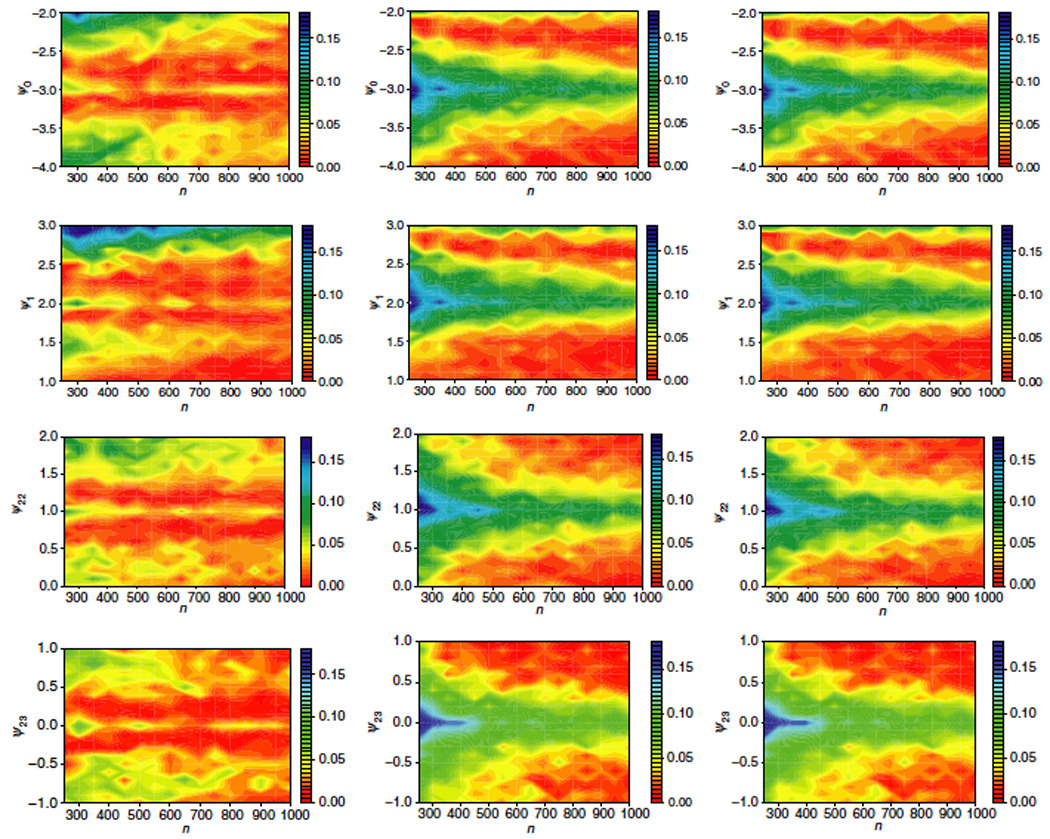
In finite samples, some misclassification of individuals into $m_j^0$ and $m_j^1$ will always occur if type I error is held fixed and both sets are non-empty. In this context, a type I error consists of falsely classifying subject i as having a unique rule when in fact he does not: $I(i\in {\hat{m}}_j^1|i\in m_j^0)$. Correspondingly, type II error is the incorrect classification of subject i as having a non-unique optimal regime when in truth his optimal rule is unique: $I(i\in {\hat{m}}_j^0|i\in m_j^1)$. An unfortunate consequence is that ZIPI introduces bias where none exists using ordinary recursive g-estimation in regions of the parameter space that are moderately close to the exceptional laws (Figure 3); see section 3.3 for further explanation of this phenomenon. As sample size increases, the magnitude of the bias and the region of “moderate proximity” to the exceptional law, where bias is observed, decrease. The maximum bias observed using ZIPI is smaller than the bias observed using usual g-estimation: 0.033 with 80% confidence interval (CI) selection and 0.040 with 95% CI selection as compared to 0.060 with g-estimation (Figure 1, Figure 3–Figure 4).

Figure 3.

Absolute bias of ψ̂₁₀ as sample size varies at and near exceptional laws using Zeroing Instead of Plugging In (ZIPI) when 95% confidence intervals suggest exceptional laws. In each figure, one of ψ₂₀, ψ₂₁, ψ₂₂, ψ₂₃ is varied while the other three parameters are fixed at −3.0, 2.0, 1.0, or 0.0, respectively.

Figure 4.

Absolute bias of ψ̂₁₀ as sample size varies at and near exceptional laws using Zeroing Instead of Plugging In (ZIPI) when 80% confidence intervals suggest exceptional laws. In each figure, one of ψ₂₀, ψ₂₁, ψ₂₂, ψ₂₃ is varied while the other three parameters are fixed at −3.0, 2.0, 1.0, or 0.0, respectively.

ZIPI falls into the class of pre-test estimators that are frequently used in a variety of statistical settings (variable or model selection constitutes a common example). The ZIPI procedure requires a large number of correlated significance tests, since the algorithm requires a testing of all individuals at all intervals but the first. Control of the type I error under multiple testing has been well-studied, however many methods of controlling family-wise error rate significantly reduce the power of the tests. The false discovery rate (FDR) of Benjamini & Hochberg (1995) provides a good alternative that has been shown to work well for correlated tests (Benjamini & Yekutieli, 2001). However even in better-understood scenarios, the optimal choice of threshold is a complicated problem; see, for example, Giles et al. (1992) or Kabaila & Leeb (2006).

3.3 Consistency and asymptotic bias of ZIPI estimators

ZIPI estimators are similar to ordinary g-estimators at non-exceptional laws, with the added benefit of reduced asymptotic bias at exceptional laws.

Theorem 1

Under non-exceptional laws, ZIPI estimators converge to the usual recursive g-estimators and therefore are asymptotically consistent, unbiased, and normally distributed.

The proof is trivial. Of greater interest is the performance of ZIPI estimators under exceptional laws. We begin assuming that $m_j^0$ and $m_j^1$ are known for all j.

Theorem 2

When the distribution is exceptional and $m_j^0,m_j^1$ are known at every interval, ZIPI estimators are asymptotically consistent, unbiased, and normally distributed.

Proof

The statement is proved for the singly-robust [equation (2)] in a two-interval context. The generalization to K intervals or to the use of equation (1) follows readily.

Decompose the usual first-interval g-estimation function into two components:

$${\mathrm{\mathbb{P}}}_n(U_1^{*}({\psi }_1,{\hat{\psi }}_2))=\frac{1}{n}{\displaystyle \sum _{i=1}^n{U}_{1i}^{*}({\psi }_1,{\hat{\psi }}_2)=\frac{1}{n}{\displaystyle \sum _{i\in m_2^0}{U}_{1i}^{*}({\psi }_1,{\hat{\psi }}_2)+\frac{1}{n}{\displaystyle \sum _{i\in m_2^1}{U}_{1i}^{*}({\psi }_1,{\hat{\psi }}_2).}}}$$

For $i\in m_2^1$, g₂(l̄_2,i, a_1,i; ${\psi }_2^{†}$) ≠ 0 and so $E\left[\frac{1}{n}{\displaystyle {\sum }_{i\in m_2^1}{U}_{1i}^{*}({\psi }_1^{†},{\hat{\psi }}_2)}\right]=0$. For $i\in m_2^0$, on the other hand, $E[U_{1i}^{*}({\psi }_1^{†},{\hat{\psi }}_2)]\ne 0$ since

$$H_{1,i}({\psi }_1,{\hat{\psi }}_2)=Y_i-{\gamma }_1(L_{1,i};{\psi }_1)+[(\hat{d_{2,i}^{\mathit{\text{opt}}}}-A_{2,i})({\hat{\psi }}_{20}+{\hat{\psi }}_{21}{L}_{2,i}+{\hat{\psi }}_{22}{A}_{1,i}+{\hat{\psi }}_{23}{L}_{2,i}{A}_{1,i})]$$

is upwardly biased for $H_{1,i}({\psi }_1,{\psi }_2^{†})$, as described in section 2.2 and by Robins (2004).

Now let $H_{1,i}^0({\psi }_1)=Y_i-{\gamma }_1(L_{1,i};{\psi }_1)$ if subject i belongs to $m_2^0$ and $H_{1,i}^0({\psi }_1)=H_{1,i}({\psi }_1,{\hat{\psi }}_2)$ otherwise. The ZIPI estimating equation [corresponding to the g-estimating equation (2)] is

$$\begin{array}{c}{U}_{1i}^{0*}({\psi }_1,{\hat{\psi }}_2)=\frac{1}{n}\{{\displaystyle \sum _{i\in m_2^0}I[g_2({\overline{L}}_2,A_1;}{\psi }_2^{†})=0]H_{1,i}^0({\psi }_1)\{S_j(A_j)-E[S_j(A_j)|{\overline{L}}_j,{\mathit{Ā}}_{j-1}]\}\hfill \\ +{\displaystyle \sum _{i\in m_2^1}(1-I[g_2({\overline{L}}_2,A_1;}{\psi }_2^{†})=0])H_{1,i}^0({\psi }_1)\{S_j(A_j)-E[S_j(A_j)|{\overline{L}}_j,{\mathit{Ā}}_{j-1}]\}\}.\hfill \end{array}$$

$E[U_{1i}^{0*}({\psi }_1,{\hat{\psi }}_2)]=0$, and therefore ZIPI estimators calculated under known $m_2^0,m_2^1$ are consistent and asymptotically unbiased for any ψ in the parameter space and at any law, exceptional or otherwise.

Of course, $m_j^0$ and $m_j^1$ are not known and must always be estimated. Typically, some misclassification will occur. Recall a type I error is that of using the estimate ψ̂₂ rather than 0 in H_1,i(ψ₁) and a type II error is that of using 0 when a plug-in estimate would have been desired. We now calculate the asymptotic bias and compare this to the result of section 2.2 to demonstrate that even when $m_j^0$ and $m_j^1$ are estimated, ZIPI exhibits less asymptotic bias than recursive g-estimation. As with ordinary g-estimation, generalization of the expression for the asymptotic bias for K > 2 intervals is not trivial because of the need to use both regular and asymptotically biased plug-in estimates.

Theorem 3

When the distribution law is exceptional and $m_2^0,m_2^1$ are estimated, two-interval ZIPI estimators have smaller asymptotic bias than the usual recursive g-estimators provided estimates are not shared across intervals, and $\underset{{\overline{L}}_2,A_1}{\text{inf}}\{|g_2({\overline{L}}_2,A_1;{\psi }_2^{†})|\}\backslash \{0\}=\mu >0$.

Proof

Since $|g_2({\overline{L}}_2,A_1;{\psi }_2^{†})|\ge \mu$ for some μ > 0 for all subjects with a unique optimal rule at the second interval, it follows that there exists a sample size such that the power to detect whether $g_2({\overline{L}}_{2,i},A_{1,i};{\psi }_2^{†})\ne 0$ is effectively equal to 1 if classification of individuals into $m_2^0,m_2^1$ is performed using 1 − ε confidence intervals for fixed type I error ε. However, 100ε% of the people with non-unique treatment rules will be falsely classified as belonging to ${ℳ}_2^1$.

Assume linear blips, so ${\psi }_2^{†}·X_2=0$ when laws are exceptional, where the true values of ψ₁, ψ₂ are denoted by ${\psi }_1^{†},{\psi }_2^{†}$. Define ${\mathrm{\Delta }}_1^z({\hat{\psi }}_2,{\psi }_2^{†})=U_1^{0*}({\psi }_1,{\hat{\psi }}_2)-U_1^{0*}({\psi }_1,{\psi }_2^{†})$, a quantity in ZIPI estimation similar to ${\mathrm{\Delta }}_1^g({\hat{\psi }}_2,{\psi }_2^{†})$ in the usual g-estimation procedure. Since, asymptotically, the only form of misclassification error in ZIPI is type I, ${\mathrm{\Delta }}_1^z({\hat{\psi }}_2,{\psi }_2^{†})$ consists of three components:

1. If $i\in m_j^0$ and $i\in {\hat{m}}_j^0$, ${\mathrm{\Delta }}_1^z({\hat{\psi }}_2,{\psi }_2^{†})=0$;

2. If $i\in m_j^0$ and $i\in {\hat{m}}_j^1$,

   $${\mathrm{\Delta }}_1^z({\hat{\psi }}_2,{\psi }_2^{†})=\{S_1(A_1)-E[S_1(A_1)|L_1]\}·(I[({\hat{\psi }}_2-{\psi }_2^{†})·X_2>0]-A_2)({\hat{\psi }}_2-{\psi }_2^{†})·X_2$$

   ;
3. If $i\in m_j^1$,

   $$\begin{array}{c}{\mathrm{\Delta }}_1^z({\hat{\psi }}_2,{\psi }_2^{†})=\{S_1(A_1)-E[S_1(A_1)|L_1]\}\hfill \\ \times \{(I[g_2({\overline{L}}_2,A_1;{\hat{\psi }}_2)>0]-A_2)g_2({\overline{L}}_2,A_1;{\hat{\psi }}_2)-(I[g_2({\overline{L}}_2,A_1;{\psi }_2^{†})>0]-A_2)g_2({\overline{L}}_2,A_1;{\psi }_2^{†})\}\hfill \end{array}$$

   .

Similar to the calculation of section 2.2, the asymptotic bias of ψ̂₁ is proportional to $E[{\mathrm{\Delta }}_1^z({\hat{\psi }}_2,{\psi }_2^{†})]$. The classification procedure in ZIPI incorrectly fails to use zeros for 100ε% of the sample with ${ℳ}_1^0$. Therefore we rewrite ${\mathrm{\Delta }}_1^z({\hat{\psi }}_2,{\psi }_2^{†})$ in terms of ${\mathrm{\Delta }}_1^g({\hat{\psi }}_2,{\psi }_2^{†})$ of recursive g-estimation:

$$\begin{array}{cc}E[\sqrt{n}{\mathrm{\mathbb{P}}}_n{\mathrm{\Delta }}_1^z({\hat{\psi }}_2,{\psi }_2^{†})]=\hfill & \epsilon E[\sqrt{n}{\mathrm{\mathbb{P}}}_{n}I[g_2({\overline{L}}_2,A_1;{\psi }_2^{†})=0]{\mathrm{\Delta }}_1^g({\hat{\psi }}_2,{\psi }_2^{†})]\hfill \\ \hfill & +E[\sqrt{n}{\mathrm{\mathbb{P}}}_{n}I[g_2({\overline{L}}_2,A_1;{\psi }_2^{†})\ne 0]{\mathrm{\Delta }}_1^g({\hat{\psi }}_2,{\psi }_2^{†})].\hfill \end{array}$$

It follows directly that the asymptotic bias of first-interval ZIPI estimates at exceptional laws is

$$-\epsilon {\left(E\left[\frac{\partial }{\partial {\psi }_1}{U}_1^{*}({\psi }_1^{†},{\psi }_2^{†})\right]\right)}^{-1}E[I[g_2({\overline{L}}_2,A_1;{\psi }_2^{†})=0]\{S_1(A_1)-E[S_1(A_1)|L_1]\}{(2\pi )}^{-1/2}{(X_2^{\prime }{\mathrm{\Sigma }}_2{X}_2)}^{1/2}].$$

In finite samples both type I and type II error will be observed, which leads to additional bias in the ZIPI estimates. When sample size is not sufficient for power to equal 1, ${\mathrm{\Delta }}_1^z({\hat{\psi }}_2,{\psi }_2^{†})$ is decomposed into four components (two of which are zero in expectation). If type II error is denoted by β, then, approximately, for two-intervals the bias will be proportional to

$$\begin{array}{c}\epsilon \mathrm{P}(g_2({\overline{L}}_2,A_1;{\psi }_2^{†})=0)E[{\mathrm{\Delta }}_1^g({\hat{\psi }}_2,{\psi }_2^{†})]+\beta \mathrm{P}(g_2({\overline{L}}_2,A_1;{\psi }_2^{†})\ne 0)\hfill \\ \times E[\{S_1(A_1)-E[S_1(A_1)|L_1]\}(I[g_2({\overline{L}}_2,A_1;{\psi }_2^{†})>0]-A_2)g_2({\overline{L}}_2,A_1;{\psi }_2^{†})].\hfill \end{array}$$

When covariates are integer-valued as in our simulations, there is good separation of g₂(L̄₂, A₁; ψ̂₂) between those people with unique rules and those without; in this instance, simulations suggest that choosing a relatively large (e.g., 0.20) type I error provides a good balance between bias reduction at and near exceptional laws (Figure 3–Figure 4). In general, we expect that it is preferable to have low type II error rather than low type I error. When a type I error is made, the ZIPI procedure will incorrectly assume an individual does have a unique regime and fail to plug in a zero, making the ZIPI estimate numerically more similar to the usual g-estimate, which is known to be unbiased (though not asymptotically so). When a type II error is made, the individual is incorrectly believed to have non-unique optimal rules at the second stage. $H_{1,i}^0({\psi }_1,{\hat{\psi }}_2)$ and H_1,i(ψ₁, ψ̂₂) will be equal only if individual i happened to receive the optimal treatment at the second interval, and so the impact of the misclassification resulting from type II error will depend on the distribution of treatments at the second interval.

3.4 ZIPI versus simultaneous (non-recursive) g-estimation

With ZIPI g-estimation proving both theoretically and in simulation to be asymptotically less biased than recursive g-estimation when parameters are not shared between intervals, it is a natural choice. The assumption of unshared parameters is in many cases appropriate, even when the number of intervals is large. For example, when studying the effect of breastfeeding in infant growth, blips at different intervals are not expected to share parameters as effects are thought to vary by developmental stage of infancy (Kramer et al., 2004). However, it is plausible that blip functions for a treatment given over several intervals for a chronic condition may share parameters. The question then arises as to whether ZIPI outperforms simultaneous (non-recursive) g-estimation.

If parameters are shared across intervals, that is, ψ_j = ψ_j′ for some j ≠ j′, recursive methods may still be used by pretending otherwise, using a recursive form of g-estimation (the usual or ZIPI) then averaging the interval-specific estimates of ψ^†. Such inverse covariance weighted recursive g-estimators have the advantage of being easier to compute than simultaneous estimators and are also doubly-robust under non-exceptional laws (Robins 2004, p. 221); note that the definition of exceptional laws is the same whether or not parameters are assumed to be shared. On the other hand, simultaneous g-estimation searches for estimates of the shared parameters directly without needing to average estimates from different intervals.

Robins (2004, p. 221–222) recommends simultaneous g-estimation for non-exceptional laws when there are few subjects who change treatment from one interval to the next: with few changes of treatment at a particular interval j, estimates ψ̂_j are extremely variable. If there are a moderate number of treatment changes from one interval to the next (recursive) ZIPI estimation may be useful for the purposes of bias reduction in large samples. Figure 5 compares ZIPI with 80% confidence intervals used to estimate membership in $m_j^0$ or $m_j^1$, recursive g-estimation, and simultaneous g-estimation, for varying sample sizes, for data as before: L₁ ~ 𝒩(0, 3); L₂ ~ round(𝒩(0.75, 0.5)); Y ~ 𝒩(1, 1)−|γ₁(L₁, A₁)|−|γ₂(L̄₂, Ā₂)| but we now impose stationarity so that γ₁(L₁, A₁) = A₁(ψ₀ + ψ₁L₁) and γ₂(L̄₂, Ā₂) = A₂(ψ₀ + ψ₁L₂ + ψ₂₂A₁ + ψ₂₃L₂A₁). Note the sharing of ψ₀ and ψ₁ between the blips of both intervals.

Figure 5.

Absolute bias in ψ̂₀ as n varies about exceptional laws assuming stationarity: inverse-covariance weighted ZIPI estimates with 80% CIs, inverse-covariance weighted recursive g-estimates, and simultaneous g-estimates [left, center, and right columns]. Rows: the true value of one of ψ₀, ψ₁, ψ₂₂, ψ₂₃ is varied; the rest are fixed at −3.0, 2.0, 1.0, or 0.0, respectively.

In our simulations, simultaneous and recursive g-estimation are similar in terms of both bias and variability. Relative to simultaneous g-estimation, the recursive methods are easier to implement and do not suffer from the possibility of multiple roots under linear blip functions. At non-exceptional laws, ZIPI produces nearly identical estimates to the doubly-robust recursive g-estimation which, as noted above, is locally efficient. In our simulations, ZIPI’s performance at exceptional laws varied by situation, performing much better when ψ₁ = 2 as compared to when ψ₁ = 3 (Figure 5), indicating that inverse-covariance weighted ZIPI estimators are not always less biased than simultaneous g-estimators.

3.5 ZIPI versus Iterative Minimization for Optimal Regimes

It is worth noting that the asymptotic bias due to exceptional laws is also present in the Iterative Minimization for Optimal Regimes (IMOR) (Murphy, 2003) method as well. This is not surprising since IMOR and g-estimation are very closely related (Moodie et al., 2007). As observed with the usual g-estimation, ZIPI outperforms IMOR when parameters are not shared across intervals (Table 4). Nevertheless, when parameters are shared and the sample is not very large, IMOR may prove to be less biased at exceptional laws than ZIPI, as in the previous subsection.

Table 4.

Parameter estimates under exceptional laws: summary statistics of g-estimation using Zeroing Instead of Plugging In (ZIPI) and the IMOR from 1000 datasets of sample sizes 250, 500 and 1000 using 80% CIs for ZIPI.

		ZIPI				IMOR
n	ψ†	Mean(ψ̂)	SE	rMSE	Cov.a	Mean(ψ̂)	SE	rMSE	Cov.a
250
	ψ10 = 1.6	1.628	0.167	0.233	93.3	1.643	0.193	0.259	95.9
	ψ11 = 0.0	0.002	0.042	0.058	93.6	−0.002	0.043	0.059	92.7
	ψ20 = −3.0	−3.017	0.296	0.409	92.4	−3.042	0.391	0.524	95.7
	ψ21 = 2.0	2.011	0.325	0.451	92.1	2.040	0.381	0.516	94.1
	ψ22 = 1.0	1.022	0.442	0.606	94.6	1.046	0.496	0.675	94.4
	ψ23 = 0.0	−0.020	0.507	0.693	94.9	−0.047	0.516	0.699	95.1
500
	ψ10 = 1.6	1.625	0.118	0.160	95.0	1.640	0.137	0.180	96.7
	ψ11 = 0.0	0.000	0.030	0.041	94.4	0.000	0.030	0.041	94.6
	ψ20 = −3.0	−2.993	0.212	0.288	93.4	−2.997	0.276	0.369	95.5
	ψ21 = 2.0	1.995	0.234	0.319	93.6	2.000	0.269	0.362	94.5
	ψ22 = 1.0	0.994	0.313	0.419	95.7	1.000	0.349	0.470	96.0
	ψ23 = 0.0	0.009	0.361	0.482	95.8	0.002	0.363	0.488	96.3
1000
	ψ10 = 1.6	1.608	0.083	0.116	92.7	1.619	0.097	0.129	95.3
	ψ11 = 0.0	0.000	0.021	0.028	96.2	0.000	0.021	0.028	96.2
	ψ20 = −3.0	−3.010	0.151	0.206	93.8	−3.020	0.197	0.265	95.9
	ψ21 = 2.0	2.009	0.166	0.227	94.0	2.017	0.191	0.258	95.2
	ψ22 = 1.0	1.015	0.222	0.305	94.0	1.023	0.249	0.342	94.0
	ψ23 = 0.0	−0.013	0.256	0.347	94.0	−0.018	0.258	0.353	94.3

^aCoverage of 95% Wald confidence intervals

4 Discussion

In this paper, we have discussed the asymptotic bias of optimal decision rule parameter estimators in the presence of exceptional laws. We also presented suggestions to reduce the computational burden of trying to detect exceptional laws using the method of Robins (2004). We introduced Zeroing Instead of Plugging In, a recursive form of g-estimation, that is to be preferred over recursive g-estimation whenever parameters are not shared between intervals if there is a possibility of laws being exceptional.

The ZIPI algorithm provides an all-or-nothing adjustment, using weights of zero or one for each individual depending on the estimated unique-rule class membership. Other approaches to bias reduction were considered, including weighting by each individual’s probability of having a unique optimal rule, but the improvement in the estimates was unremarkable. We will pursue other methods such as, for example, weighted averaging of the ZIPI and usual g-estimates in the pursuit of a method that works well both with shared and unshared parameters. The efficacy of the ZIPI procedure has not been tested in the case of non-linear blip functions for, say, estimating the optimal rules for a binary outcome. This, too, shall be investigated.

Future work will also include determination of the optimal choice of threshold in ZIPI; simulations suggest that when there is reasonably good separation of people with unique rules and those without, a relatively large probability of type I error (e.g., 0.20) works well. When the distinction between those individuals with unique rules and those without is smaller, controlling the type I error in the class-membership testing through the false-discovery rate or a comparable procedure may be desirable. We will also investigate using the ZIPI procedure with type I error that systematically decreases with increasing sample size while maintaining high power to detect individuals with unique optimal rules.

Oetting et al. (2008) have performed the most comprehensive study of sample size requirements for a two-interval, two-treatment sequential multiple assignment randomized trial (SMART) (Collins et al., 2007) yet. In this study, sample size calculations were based on testing for a difference between the best and next-best strategy by considering the difference in mean response under the two treatment strategies. Earlier sample size calculations for testing between strategies were derived by Murphy (2005). To date, no thorough study has been performed for the sample size requirements for testing optimal strategies selected via g-estimation, and so the impact of parameter sharing on sample size and efficiency is not well understood. However it is assumed that the ‘reward’ for the additional assumption of shared parameters would be increased efficiency (under correct specification). A future direction of research will be the investigation of the properties of g-estimators and required sample sizes under both shared and unshared parameter assumptions.

We conclude by observing that one of g-estimation’s primary points of appeal is that, unlike traditional approaches such as dynamic programming, estimates are asymptotically unbiased under the null hypothesis of no treatment effect even if the distribution law of the complete longitudinal data is not known, provided the true law is not exceptional. However for a blip function that includes at least one component of treatment and covariate history, under the hypothesis of no treatment effect, every distribution is an exceptional law and therefore g-estimation is asymptotically biased under the null for all such blip functions and laws. Thus when primary concern is in performing a valid test of the null hypothesis of no treatment effect, we may consider fitting a “null” blip model which does not include any covariates (using the doubly robust estimator), proceeding to richer blip models only if the “null” blip model cannot be rejected.

References

- Benjamini Y, Hochberg Y. Controlling the false discovery rate: a practical and powerful approach to multiple testing. J. R. Stat. Soc. Ser. B Stat. Methodol. 1995;57:289–300. [Google Scholar]
- Benjamini Y, Yekutieli D. The control of the false discovery rate in multiple testing under dependency. Ann. Statist. 2001;29:1165–1188. [Google Scholar]
- Collins LM, Murphy SA, Strecher V. The Multiphase Optimization STrategy (MOST) and the Sequential Multiple Assignment Randomized Trial (SMART): New methods for more potent e-health interventions. American Journal of Preventative Medicine. 2007;32(5S):S112–S118. doi: 10.1016/j.amepre.2007.01.022. [DOI] [PMC free article] [PubMed] [Google Scholar]
- Giles DEA, Lieberman O, Giles JA. The optimal size of a preliminary test of linear restrictions in a misspecified regression model. J. Amer. Statist. Assoc. 1992;87:1153–1157. [Google Scholar]
- Kabaila P, Leeb H. On the large-sample minimal coverage probability of confidence intervals after model selection. J. Amer. Statist. Assoc. 2006;101:619–629. [Google Scholar]
- Kramer MS, Guo T, Platt RW, Vanilovich I, Sevkovskaya Z, Dzikovich I, Michaelsen KF, Dewey K. Feeding effects on growth during infancy. The Journal of Pediatrics. 2004;145:600–605. doi: 10.1016/j.jpeds.2004.06.069. [DOI] [PubMed] [Google Scholar]
- Moodie EEM, Richardson TS, Stephens DA. Demystifying optimal dynamic treatment regimes. Biometrics. 2007;63:447–455. doi: 10.1111/j.1541-0420.2006.00686.x. [DOI] [PubMed] [Google Scholar]
- Murphy SA. Optimal dynamic treatment regimes. J. R. Stat. Soc. Ser. B Stat. Methodol. 2003;65:331–366. [Google Scholar]
- Murphy SA. An experimental design for the development of adaptive treatment strategies. Stat. Med. 2005;24:1455–1481. doi: 10.1002/sim.2022. [DOI] [PubMed] [Google Scholar]
- Oetting AI, Levy JA, Weiss RD, Murphy SA. Statistical methodology for a SMART design in the development of adaptive treatment strategies. In: Shrout P, editor. Causality and psychopathology: finding the determinants of disorders and their cures. Arlington VA: American Psychiatric Publishing, Inc.; 2008. [Google Scholar]
- Robins JM. Correcting for non-compliance in randomized trials using structural nested mean models. Comm. Statist. Theory Methods. 1994;23:2379–2412. [Google Scholar]
- Robins JM. Causal inference from complex longitudinal data. In: Berkane M, editor. Latent variable modeling and applications to causality. New York: Springer-Verlag; 1997. pp. 69–117. [Google Scholar]
- Robins JM. Optimal structural nested models for optimal sequential decisions. In: Lin DY, Heagerty PJ, editors. Proceedings of the Second Seattle Symposium on Biostatistics; New York: Springer-Verlag; 2004. pp. 189–326. [Google Scholar]
- Robins JM, Orellana L, Rotnitzky A. Estimation and extrapolation of optimal treatment and testing strategies. Stat. Med. 2008;27:4678–4721. doi: 10.1002/sim.3301. [DOI] [PubMed] [Google Scholar]
- Rubin DB. Bayesian inference for causal effects: The role of randomization. Ann. Statist. 1978;6:34–58. [Google Scholar]
- van der Vaart A. Asymptotic Statistics. Cambridge: Cambridge University Press; 1998. [Google Scholar]