

Abstract
A Fortran program package is introduced for rapid evaluation of the electrostatic potentials and forces in biomolecular systems modeled by the linearized Poisson-Boltzmann equation. The numerical solver utilizes a well-conditioned boundary integral equation (BIE) formulation, a node-patch discretization scheme, a Krylov subspace iterative solver package with reverse communication protocols, and an adaptive new version of fast multipole method in which the exponential expansions are used to diagonalize the multipole to local translations. The program and its full description, as well as several closely related libraries and utility tools are available at http://lsec.cc.ac.cn/lubz/afmpb.html and a mirror site at http://mccammon.ucsd.edu/. This paper is a brief summary of the program: the algorithms, the implementation and the usage.
Keywords: Poisson-Boltzmann Equation, Boundary Integral Equation, Node-patch Method, Krylov Subspace Methods, Fast Multipole Methods, Diagonal Translations
1. Introduction
In the past thirty years, the Poisson-Boltzmann (PB) continuum electrostatic model has been widely accepted as a tool in theoretical studies of interactions of biomolecules such as proteins and DNAs in aqueous solutions. Recent work includes the introduction of more physical boundary conditions so that PB and its linearized version become valid for a wider class of molecular systems [38].
In this paper, we describe an adaptive fast multipole Poisson-Boltzmann (AFMPB) solver for solving the linearized PB equation, and thus for elucidating the electrostatic role in many biological processes, such as enzymatic catalysis, molecular recognition and bio-regulation. Indeed, quite a few PB solvers are available in biochemistry and biophysical communities, including DelPhi, GRASP, MEAD, UHBD and PBEQ based on the finite difference formulation [10], and APBS (Adaptive Poisson-Boltzmann Solver) based on the finite volume/multigrid framework [11, 22]. In the linearized PB regime, algorithms using the boundary integral equation (BIE) approach have shown great promise for their efficiency on scaling and memory requirements [13, 25, 28]: when Green’s theorem and potential theory are applied, the linearized PB equation can be recasted into a set of boundary integral equations where the unknowns are only de-fined on the surface of the molecule. Therefore, the number of unknowns is reduced when compared with the volumetric discretization in finite difference and finite element methods.
This AFMPB solver reflects our effort on developing more efficient codes using the BIE approach for the linearized PB equation, currently on single processor computing architectures. Several techniques are used in AFMPB to improve its efficiency over existing BIE-based solvers. First, a well-conditioned BIE formulation is used so that the number of iterations in the Krylov subspace methods is bounded, independent of the number of unknowns in the system. Second, a node-patch scheme is applied to discretize the resulting BIE, and the node based scheme reduces the number of unknowns defined on the molecular surface compared with commonly used “constant element” discretizations. Further, the iterative Krylov subspace methods from the SPARSKIT package [7] are applied to the resulting linear systems with simplified calling interface with the use of the reverse communication protocols. Fourth, the adaptive new versions of the fast multipole methods (FMMs) from FMMSuite [4] are applied to the convolution type discretized integrals. Finally, interface computer programs are provided to couple AFMPB with many existing mesh generating (e.g. MSMS [6] or other programs that can generate OFF format type of mesh) and visualization tools (e.g. VMD [5]). Preliminary numerical experiments show that the new AFMPB solver achieves significant speedup and memory savings for calculating the electrostatics of large-scale biomolecular systems on single-processor personal computers. We are currently parallelizing the codes on multi-core/multi-processor computer architectures toward simulating the dynamics of complex biomolecular systems under the influence of electrostatic forces derived from the PB calculation.
This paper is organized as follows. In Section 2, we describe various numerical techniques used in the AFMPB solver, including the boundary integral equation formulation for the linearized PB equation, the node-patch discretization, the Krylov subspace methods, and the adaptive new version of FMM. In Section 3, the overall structure of the codes is discussed, in particular, how it can be coupled with existing tools for pre- and post-processing. In Section 4, test runs are described to illustrate the performance of the solver. Finally, in the Appendix, we briefly describe the units and several important parameters used in our codes, and provide a sample shell script file for running the package.
2. Theoretical Background
2.1. Electrostatics in Biomolecular Systems
The electrostatic force is considered an important factor in understanding the interactions and dynamics of molecular systems in solution. One commonly used continuum model for describing the electrostatic effects of the solvent outside the molecules is the Poisson-Boltzmann (PB) equation
| (1) |
and the Poisson equation is used for the inside of the molecules. When electrostatic potentials are small, the linearized PB (LPB) equation
| (2) |
is valid. The LPB equation can be generalized to a wider class of problems when proper interface boundary conditions are given [38].
In numerical simulations of large molecular systems, efficient solution of the Poisson-Boltzmann equation is required, for direct visualization of electrostatic potentials, for calculating the energetics of molecular interactions in solution, and more importantly, for understanding the dynamics of molecular systems in which the PBE is coupled with time evolution equations including the continuum diffusion equations and the Newton’s law of motion.
2.2. Boundary Integral Equation Formulations
There are several ways to reformulate the LPB equation as “boundary integral equations”. When Green’s second identity is applied directly, the traditional boundary integral equations for the linearized PB equation for a single domain (molecule) takes the form
| (3) |
with the interface conditions φint = φext and . In the formulas, is the interior potential at surface position p of the molecular domain Ω, S = ∂Ω is its boundary, i.e., solvent-accessible surface, is the exterior potential at position p, Dint is the interior dielectric constant, t is an arbitrary point on the boundary, n is the outward normal vector at t, ∮ represents the principal value integral to avoid the singular point when t → p in the integral equations, and are the fundamental solutions of the corresponding Poisson and linearized Poisson-Boltzmann equations, respectively, rk is the position of the kth source point charge qk of the molecule, and κ is the reciprocal of the Debye-Hückel screening length determined by the ionic strength of the solution. Unfortunately, this “natural” boundary integral equation formulation is in general a Fredholm integral equation of the first kind and hence ill-conditioned. When solved iteratively using the Krylov subspace methods, the number of iterations increases with the number of unknowns. The resulting algorithm becomes inefficient for large systems.
In our AFMPB solver, instead of simply accepting this natural BIE formulation, we use the technique in [33] and combine the single and double layer potentials to derive a second kind Fredholm integral equation as in (with notations f = φext, )
| (4) |
where n0 is the unit normal vector at point p ∈ S. This is a well-conditioned (Fredholm second kind) system of equations. When Krylov subspace methods are applied to such systems, the number of iterations remains bounded even for a large number of unknowns. Similar formulations are also used in [24] where a complete boundary integral equation formulation is derived for the linearized PB equation using a limiting process to avoid the singularity problem, and in later boundary element method (BEM) based PB work [13, 27, 36].
2.3. “Node-patch” Discretization
To discretize Eqs. (4), one commonly used technique in engineering community is the “constant element” approach that triangularizes the molecular surface and treats the unknowns as constants on each triangular element. In this approach, the number of unknowns equals to the number of elements. Alternatively, the “linear element” method linearly interpolates the solution using the three constituent nodes, therefore the number of unknowns equals to the number of nodes. As there are less number of nodes than surface elements, the linear element approach leads to a reduction of the total number of unknowns by approximately a factor of 2. However, the node-based linear element approach introduces additional complexity in its implementation. In the AFMPB solver, we develop a “node-patch” approach to take advantage of the easy implementation of the constant element method and the reduced number of unknowns in the linear element method.
The idea of the node-patch approach is to construct a “working” patch around each node instead of directly using the facet patch (element), and assume that the unknowns are constants on each new “node-patch”. These new patches are illustrated in Figure 1, in which a “node-patch” is constructed around the ith node that has five neighboring elements. The new patch is defined by the area encircled by a set of points {O1,C1, O2,C2, ···, O5,C5, O1}, where {Ol, l = 1, ···, 5} are the centroids of the five adjacent triangles, and {Cl, l = 1, ···, 5} are the midpoints of the five joint edges. Clearly, each triangular element contributes one-third of its area to the new node-patch. Therefore, for far-field integration using fast multipole method the charge on the patch can be approximated by the unknown ( f or h) at the node multiplied by the total area of the node-patch (see ref. [30] for more details), while for near-field a normal quadrature method is used as in the constant or linear element method.
Figure 1.
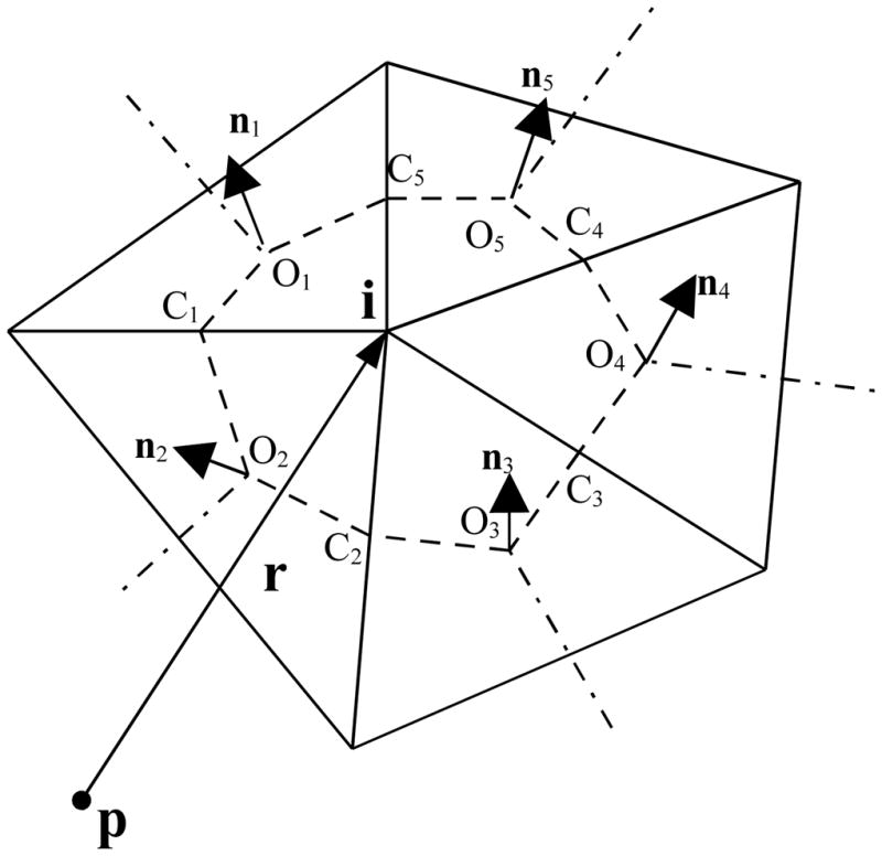
“Node” patch constructed on a triangular mesh. O and n are the centroid and normal vector of an element respectively, and C is the middle point of an edge.
There are several advantages of this “node-patch” approach. First, because of the reduction of the total number of unknowns when compared to the constant element method, the computational cost of solving the resulting linear system is accordingly reduced. The “node-patch” method does involve an additional preprocessing step for deriving the average charge on each patch. This, however, only constitutes a negligible portion of the total computation time, and the processed geometric coefficients can also be saved for repeated use in iterative solving procedures. Second, relative to the linear element method, the “node-patch” method is significantly more efficient in searching and indexing the local list when used with practical matrix storage formats such as the Harwell-Boeing sparse matrix format or modified sparse column (row) format. Finally, in the “node-patch” method, as in the constant element method, the source and target are the same - the nodes, making the application of FMM from the FMMSuite package straightforward.
2.4. Krylov Subspace Methods
Given an initial iterate x0, the Krylov subspace method solves the linear system Ax = b by iteratively minimizing some measure of error over the space x0 + Kk, where Kk = span{r0, Ar0, A2r0, ···, Ak−1r0} and r0 is the initial residual usually defined as r0 = b − Ax0. Based on different measures of the error and different types of matrices, there are many different Krylov subspace method implementations. As the matrix A after the node-patch discretization is non-symmetric and there is no fast algorithm to apply the transpose of A to an arbitrary vector, we adopt four different Krylov iterative subroutines from the open source package SPARSKIT developed by Saad and collaborators [7], including the full GMRES, the restarted GMRES, the biconjugate gradients stabilized (BiCGStab) method, and the transpose free QMR (TFQMR). Since Eq. (4) is a well-conditioned Fredholm second kind integral equation system and the corresponding operator consists of an identity operator plus a compact operator whose eigenvalues only cluster at 0, the number of iterations in the Krylov subspace methods is therefore bounded, independent of the number of nodes in the discretization. Preliminary numerical experiments show that the full GMRES method converges faster than the other methods, which agrees with existing analysis. Because the memory required by the GMRES method increases linearly with the iteration number k, and the number of multiplications scales like , for large k, the GMRES procedure becomes very expensive and requires excessive memory storage. For these reasons, instead of a full orthogonalization procedure, GMRES can be restarted every k0 steps where k0 < N is some fixed integer parameter. The restarted version is often denoted as GMRES(k0). The storages required by the BiCGStab and TFQMR algorithms are independent of the iteration number k, and the number of multiplications grows only linearly as a function of k. The choice of Krylov iterative solvers is problem dependent, and GMRES is chosen as the default solver in AFMPB.
An interesting feature of the iterative solvers in SPARSKIT is the so-called “reverse communication protocol” (check the ITSOL directory in SPARSKIT [7]), which avoids calling the matrix vector product subroutine from inside the Krylov solver. Instead, the Krylov solver provides a vector and asks for the matrix vector multiplication result as a further input. Therefore, it is unnecessary to pass the parameters in the FMM subroutines to the Krylov solvers, leading to easier interface between FMM and SPARSKIT, and easier memory management.
2.5. Adaptive Fast Multipole Methods
As the total number of operations required to solve Eq. (4) is a constant (representing the number of iterations) times the amount of work required for a matrix vector multiplication, when the new versions of fast multipole methods (FMMs) are applied, the matrix vector product only requires O(N) operations, therefore the linear equation system can be solved in asymptotically optimal O(N) time.
The fundamental observation in the multipole expansion based methods is that the numerical rank of the far field interactions is relatively low and hence can be approximated by P terms (depending on the prescribed accuracy) of the so-called “multipole expansion”. For the Coulomb interactions (Poisson Equation),
| (5) |
where the multipole coefficients are computed by
| (6) |
The spherical harmonic function of order n and degree m is defined according to the formula[8]
| (7) |
and is the associated Legendre polynomial. For the Debye-Hückel (screened Coulombic) interaction, a similar expansion can be written as
| (8) |
The multipole coefficients are given by
| (9) |
where in(r) and kn(r) are the modified spherical Bessel and modified spherical Hankel functions, respectively, defined in terms of the conventional Bessel function via ([8]) Iv(r) = i−vJv(ir), , and .
For arbitrary distributions of particles, a hierarchical oct-tree (in 3D) is generated so each particle is associated with boxes at different levels, and a divide-and-conquer strategy is applied to account for the far field interactions at each level in the tree structure. In the “tree code” developed by Appel[9], and Barnes and Hut [12], as each particle interacts with 189 boxes in its “interaction list” through P terms of multipole expansions at each level and there are O(logN) levels, the total amount of operations is approximately 189P2N logN. The tree code was later improved by Greengard and Rokhlin in 1987 [19]. In their original FMM, local expansions (under a different coordinate system) were introduced to accumulate information from the multipole expansions in the interaction list,
| (10) |
where are the local expansion coefficients, and for the screened Coulombic interaction, a similar expansion can be written as
| (11) |
As the particles only interact with boxes and other particles at the finest level, and information at higher levels is transferred using a combination of multipole and local expansions, the original FMM is asymptotically optimal O(N). However, because the multipole to local translation requires prohibitive 189P4 operations for each box, the huge prefactor makes the original FMM less competitive with the tree code and other FFT based methods. In 1997, a new version of FMM was introduced by Greengard and Rokhlin [20] for the Laplace equation, in which exponential expansions are introduced to diagonalize the multipole-to-local translations, and a merge-and-shift technique is used to further reduce the number of such translations. Compared with the original FMM, the original 189P4 operations were reduced to 40P2 + 6P3 in the new version. Numerical experiments show that the new version of FMM breaks even with direct calculation when the number of particles n = 500 for three digit accuracy, and n = 1000 for six digits for the screened Coulomb interactions. In our AFMPB solver, the new version of FMM was implemented for the Laplace and linearized PB equations for the efficient calculation of electrostatic interactions. As far as we know, this is the only LPB solver using the new versions of FMMs.
Instead of discussing technical details of the adaptive new version of FMM, we refer the readers to existing literature. The new version of FMM was introduced in [20] for the Laplace equation; the corresponding adaptive version was discussed in [14]; the new version of FMM for the linearized PB equation (also called Yukawa or modified Helmholtz equation) was discussed in [18, 23].
2.6. Force and Torque Calculations
For an interacting molecular system, AFMPB can also calculate the total force and torque acting on each molecule. The force is obtained through computing the stress tensor in ionic solution[17]
| (12) |
where E is the electrostatic field, δi j is the Kronecker delta function.
To obtain the boundary stress tensor, the gradient of the potential (the negative of E on the boundary) should be computed. In our current implementation, we first use an interpolation method to construct a continuous potential function f (x,y,z) in the vicinity of the molecular surface based on the PB solutions, then compute the gradient of f for any positions on the molecular surface. For more details on the interpolation method and the force calculations, we refer interested readers to [30].
Finally, the PB force F and torque M acting on any constituent molecule are calculated by integrations
| (13) |
| (14) |
where rc(x) is a vector from the center of mass of the target molecule to the surface point x, and the dot and cross vector multiplications are applied to the vector and tensor quantities.
3. Code Structure and Implementation
In this section, we describe the package portability and installation, flow chart, job running, file format and I/O layers, pre- and post-processing, and several related tools.
3.1. Portability and Installation
The software package was implemented mostly in Fortran77. Memory allocation features from Fortran 90 and above are used in a few subroutines for memory management.
After the user downloads the package and extracts it to a local computer, the following directories can be found:
Doc: contains the references and this manual.
job-examples: contains a README file, samples of the c-shell job files job.csh to run the package, and the generated input/output files. A subdirectory ./Two-proteins contains similar input/output files but is for the test case of a two-molecule system.
FBEM: the driver and the boundary integral equation codes of the AFMPB package. It also contains the subroutine iters.f, the Krylov subspace iterative solvers from SPARSKIT [7]. The default Krylov solver is GMRES, though the user can also use the restarted GMRES, TFQMR, or BiCGStab.
fmm3d_node: the fast multipole method library for the Laplace and Yukawa potentials.
tools: pre- and post- processing utility programs. Additional tools will be added to this directory for calculation of different parameters.
For compiling, check the file Makefile for further information. The package has been successfully compiled using the Intel©compiler for Linux, and the GNU©F95 compiler.
3.2. Flow Chart
The program diagram is shown in Fig. 2.
Figure 2.
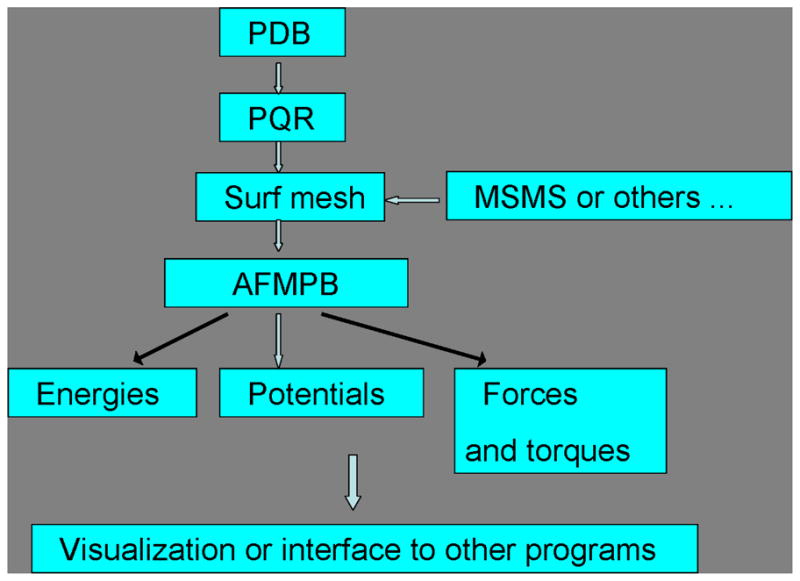
AFMPB flow chart
AFMPB can be considered as a main driver for calculating the electrostatics in biomolecular systems. It requires molecular structure, charge and mesh information from the pre-processing tools as inputs, and outputs potential, various energies and force results for visualization and/or further processing. To generate the “boundary elements”, AFMPB currently accepts mesh data from the package MSMS [6] and other programs that can generate molecular surface mesh in the OFF format. For postprocessing, we use VMD for visualization. The solver can also be coupled with multi-scale time stepping schemes to simulate the dynamics of molecular systems under the influence of electrostatic interactions.
3.3. Job running
A command line style is adopted to run AFMPB. A simple way to run AFMPB is ”./afmpb”, with all the default input/output files in the working directory. A typical job with specified options can be like
afmpb -i inp.dat -o out.log -s surfpot.dat.
-i means to be followed by the input file, -o an output log file, and -s is followed by an output file that contains surface nodal potential. More options see Appendix C.
3.4. File Formats and I/O Layer
To run AFMPB, users are required to prepare input files including (a) a control file (inp.dat by default), (b) PQR file(s) containing atomic charges and their locations, (c) molecular surface mesh file(s), and an optional (d) off-surface points location file where the potentials need to be evaluated. For the output, a log file (out.log by default) will be generated automatically after every AFMPB run, and users may also request a surface potential file (default surfpot.dat) by setting a write-control parameter in inp.dat. All the input files and output log file (out.log) are in free format. The job-control input file can also be generated by the job shell script as described in Appendix C, in which a brief explanation for each variable is provided.
The PQR format is a modification of the PDB format which adds charge and radius parameters to existing PDB file. The surface mesh file contains node coordinates and how they connect to form triangles. The current version of AFMPB allows a few slightly different mesh formats, including the standard OFF format and the so-called MSMS format. A comment line in inp.dat
“# meshfmt: 0 icosohedron, 1 raw, 2 msms, 3 matlab sphere, 4 mc, 5 off”
indicates to choose one of the optional mesh formats to be read. The OFF format is used by many mesh generating tools, and can be viewed using visualization software such as “GEOMVIEW”, while the MSMS format can be conveniently generated by using a script tool provided in our package (see the section “Utility Tools”). The script will call the software MSMS[6] that is widely used in biomolecular studies. A sample MSMS format file is as follows:
5358 10712
−18.162 1.138 29.523 −0.309 −0.779 0.546
−17.185 −0.033 30.761 −0.960 0.001 −0.280
…
16.334 2.571 23.760 −0.000 1.000 0.000
1 5 3645
3645 5 3646
…
3614 3620 3613
In this file, the first line describes the total numbers of nodes and triangular elements. Starting from the second line, the xyz coordinates and optional xyz components of the normal direction for each node are given, followed by a list indicating the indices of three nodes for each triangular element.
The AFMPB solver requires that the normal vectors point outward (as defined in the current OFF and MSMS formats) and the nodes are ordered counter-clockwisely. In case the normal vectors are not available in the input surface mesh files, which happens when other file formats are used as input files, functions are provided in the solver to calculate these quantities.
The output log file out.log records useful information during code execution, including the number of iterations of the iterative Krylov solver, the CPU time and memory usage information, the total/solvation/interaction/Coulombic energies, and so on. The surface potentials and forces are recorded in a formatted file (surfpot.dat), which can be extracted for further analysis, and can be visualized with VMD using a provided TCL script file (see the subsection “Utility Tools”).
3.5. Pre-processing
The PQR file can be generated from a standard PDB file using the software pdb2pqr [3]. pdb2pqr also adds missing hydrogen atoms in the PDB file, optimizes the hydrogen bond network, and assigns atomic charges and radii based on various force field parameter sets.
The molecular surface mesh file is traditionally generated from the PQR file. There exist at least three types of “molecular surface” to define the boundary between the low (interior) and high dielectric (exterior) regions: the van der Waals surface, the solvent-accessible surface[32], and the solvent-excluded surface. The van der Waals surface is the union of the surface area formed by placing van der Waals spheres at the center of each atom in a molecule. When rolling a solvent (or a probe) sphere over the van der Waals surface, the trajectory of the solvent sphere center defines the solvent-accessible surface, while the trajectory of the boundary of the solvent sphere in closest contact with the van der Waals surface defines the solvent-excluded surface. The solvent-excluded surface is also referred to as the molecular surface in bimolecular studies. In the AFMPB solver, a triangular mesh of the molecular surface can be generated using the software MSMS as described in [35]. Two important parameters in MSMS are the node density and probe radius that control the resolution of the output mesh, and the typical values are set to 1.0/Å2 and 1.5 Å, respectively. The mesh from MSMS can be further improved by removing the elements of extremely small area using a mesh checking procedure provided in the AFMPB package, though this step is usually not necessary. We want to mention that mesh generation is in general a fast step and takes only a few seconds for medium-sized molecules. A typical mesh of a molecule with 8362 atoms is shown in Fig 3, which contains 32975 vertices and 65982 triangles and is generated within 3 seconds of CPU time. For larger molecules or molecular assemblies, however, our numerical experiments show that almost all existing mesh generating tools fail to generate reasonable quality molecular surface meshes required for numerical stability. The mesh generation therefore remains a bottleneck for large-scale PB calculation and full scale dynamics simulations with PB forces.
Figure 3.

A typical surface triangulated mesh of a protein (Acetylcholinsterase).
3.6. Post-processing
The calculation results for energies and forces (between molecules) can be extracted from out.log. The surface and off-surface potential files can be used for further analysis. The solvation energies for individual molecules are also stored in out.log if the corresponding output options are switched on in the input file inp.dat. The solvation energy is computed by solving the PBE only once, which is different from most finite difference based methods. For multi-molecule systems, the binding energy, the total forces and torques acting on individual molecules due to the other molecules (excluding itself) can also be calculated and outputed to out.log by setting the corresponding control variables in inp.dat.
3.7. Utility Tools
The directory ./tools contains tools for file format conversion, mesh generation and refinement, and data analysis and visualization. In the current release of the solver, two scripts are provided: pqrmsms.csh and showSmoothMesh.tcl. The c-shell script pqrmsms.csh generates a MSMS molecular surface mesh from a PQR file. Before using the script file, the program MSMS should be installed and the path should be correctly set. Given a PQR file (e.g. fas2.pqr in the directory), the surface mesh can be generated by running the following command:
./pqrmsms.csh fas2 1.2 1.5.
The last two variables specify the node density (in unit of 1 per Å2) and probe radius in unit of Å, respectively.
The second tool, a TCL script showSmoothMesh.tcl, is used together with the visualization program VMD to display the surface potential data file. VMD should be installed before running the script. A sample execution to visualize the fas2 structure and the resulting surface potentials follows:
vmd fas2.pqr -e showSmoothMesh.tcl -args ../job-examples/surfpot.dat.
4. Test Run Description
4.1. Spherical Cavity
To assess the performance of the AFMPB solver, we first calculate the Born solvation energy of a point charge +50e located at the center of a spherical cavity with a radius of 50 Å. The exact Born solvation energy Esolvation of the cavity is −4046.0 (energy is in kcal/mol). The surface is discretized at various resolution levels by recursively subdividing an icosahedron. Table 1 summarizes the timing results (on a Dell dual 2.0 GHz P4 desktop with 2 GB memory) along with some critical control parameters using the AFMPB solver and a direct BEM without invoking any fast algorithms (denoted by direct BEM). We noticed that regardless of the surface resolution, all the GMRES iteration steps are below 5, which numerically confirms that our formulation is well-conditioned. The CPU time for the new version of FMM increases linearly with the number of elements, while increases quadratically for the direct BEM method.
Table 1.
BEM performance on a spherical cavity case with different surface mesh sizes
| Number of Elements | Tdirect BEM (s) | TAFMPB (s) | level | Iteration steps | Esolvation (error %) | Error (%) in | |
|---|---|---|---|---|---|---|---|
| f | h | ||||||
| 320 | 0.13 | 0.18 | 2 | 5 | −4227.5 (4.5) | 6.6 | 5.6 |
| 1280 | 1.56 | 0.82 | 3 | 5 | −4134.5 (2.2) | 2.8 | 2.5 |
| 5120 | 19.67 | 3.39 | 3 | 5 | −4088.6 (1.1) | 1.4 | 1.1 |
| 20480 | 247.20 | 15.86 | 4 | 5 | −4066.5 (0.5) | 0.7 | 0.6 |
| 81920 | 3122.10 | 87.96 | 5 | 5 | −4050.6 (0.3) | 0.2 | 0.4 |
The computational accuracy of the solver improves linearly upon the refinement of the mesh scale. As shown in Table 1, when the mesh is refined to a higher level, the number of elements is quadrupled, and the size of each element (for instance, measured by the length of edges of the triangular elements) is reduced by half, the relative errors of the calculated Born solvation energy are also reduced by approximately half when compared with the analytical result.
4.2. Fasciculin
To further illustrate the AFMPB’s performance on the electrostatic calculation for proteins, we computed the electrostatic solvation energies of fasciculinII, a 68 residue protein at various mesh resolutions. The results are shown in Table 2. It shows again that the mesh size has only a small impact on the number of iteration steps, and the memory usage and CPU time increase almost linearly with the increase of surface meshes.
Table 2.
Performance for calculations on a single protein. F denotes the number of faces, V the vertices.
| Mesh | Memory (MB) | CPU (s) | Esolvation (kcal/mol) | Iteration steps |
|---|---|---|---|---|
| 9920 F, 4962 V | 73.9 | 6.7 | −556.3 | 11 |
| 12150 F, 6077 V | 86.1 | 6.8 | −542.5 | 9 |
| 15146 F, 7575 V | 118.3 | 8.0 | −536.9 | 9 |
| 18138 F, 9071 V | 144.0 | 9.2 | −527.0 | 9 |
| 21684 F, 10844 V | 177.0 | 12.5 | −524.6 | 10 |
4.3. A Two-molecule Case: Fasciculin-acetylcholinesterase System
AFMPB is also tested for a two-molecule system, the acetylcholinesterase and its inhibitor fasciculin. They are separated by 42.2 Å away by shifting the coordinates along the center-to-center direction in the original structure. The molecular surface mesh for fasciculin contains 5198 nodes and 10400 triangles, and the mesh for acetyl-cholinesterase contains 34111 nodes and 68266 triangles. In order to extract various quantities characterizing the interaction between the two molecules, AFMPB actually solves the PBE three times: two for each isolated molecule, and one for the combined two-molecule system. The total solvation energy of the system is −3663.8 kcal/mol. The electrostatic interaction energy between fasciculin and acetylcholinesterase is 0.30 kcal/mol, and the total force (in kcal/mol.Å) and torque (in kcal/mol) acting on fasciculin are (0.08, 0.14, −0.32) and (12.53, 9.95, −7.42), respectively. The total CPU time is 73 seconds on a DELL PRECISION T7400 desktop computer.
5. Conclusion
In this paper, we describe an adaptive fast multipole Poisson-Boltzmann solver for computing the electrostatics in biomolecules. The solver uses the new version of fast multipole methods and Krylov subspace methods to solve a well-conditioned boundary integral equation formulation of the linearized PB equation. Numerical experiments show that the solver is very efficient for relatively large molecules on current desktop computers. We anticipate that the AFMPB solver, when parallelized on multi-core/multi-processor large-scale computers, can be applied to the efficient simulation of the dynamics of large molecular systems.
Acknowledgments
Finally in this paper, we want to thank many of our colleagues and collaborators for their contributions and suggestions. In particular, our code uses many existing open source codes, including the SPARSKIT by Saad and collaborators [7], MSMS [6] for mesh generation, VMD [5] for visualization, and several important subroutines in the new version of FMM from Profs. Greengard and Rokhlin’s groups. This work was supported by HHMI, NIH, NBCR, NSF (JH: NSF0811130 and NSF0411920, JAM: MCB0506593), the NSF Center of Theoretical Biological Physics (CTBP), and the Institute for Mathematics and Its Applications (IMA). In addition, BL is partially funded by the Academy of Mathematics and Systems Science of Chinese Academy of Sciences, the State Key Laboratory of Scientific/Engineering Computing, and NSFC (NSFC10971218), and XC is partially supported by the U.S. Department of Energy Field Work Proposal ERKJE84. Their support is thankfully acknowledged.
Appendix
Appendix A: Units
The following table (Table 3) lists the units used in AFMPB. The conversion factors to transform to SI units are also given in the last column for reference.
Table 3.
Units in AFMPB.
| Variable | AFMPB | SI |
|---|---|---|
| Length | 1 Å | 1 ×10⁻¹⁰ m |
| Energy | 1 kcal/mol | 4186 J/mol |
| Charge | 1 electron | 1.602 ×10⁻¹⁹ C |
| Force | 1 kcal/mol-Å | 6.948−11 N |
| Ionic strength | 1 mM | 1 ×10⁻³ M |
| Temperature | K | 1 K |
| Permittivity* | 1 ε0 | 8.854 ×10⁻¹² F/m |
The relative permittivity is used in input file. ε0 is the permittivity in vacuum.
Appendix B: Important Parameters
We recommend advanced users to check the following header files for adjustable parameters used in the program.
defgeom.h: defines the variables describing the geometry of the molecules.
files.h: defines the units for various input and output files.
fmmtree.h: in the fast multipole method, the size of many variables and vectors can be determined before one knows the adaptive tree structure for an input geometry. In this file, all the “fixed” length variables are defined, including many variables for storing the precomputed data. One common block is defined in this file for the adaptive tree structure.
membem.h: defines the geometry and input/output variables in the BEM subroutines. The common block geomol defines the numbers of molecules, node points, elements, and singular charges. The common block membem defines the pointer to a huge working array where different geometry and input/output variables are stored.
memfmm.h: defines the pointers for the variables in the FMM subroutines. All adjustable variables are allocated once the adaptive tree structure is determined, and these pointers are generated for integer, real, and complex variables, respectively.
-
parm.h: defines important physical and code parameters. In particular, the following parameters are used for code control.
lw: as the tree structure is adaptive, one can not determine the size of the required memory where the oct-tree structure will be stored. Hence initially a large amount of memory space is allocated to generate the adaptive tree. If this number is too small, error message will be provided asking the user to increase this number.
nbox: in our adaptive strategy, we ask that the maximum number of particles in each childless box is less than nbox. Reducing this parameter will generate more levels (which means more boxes but less direct interactions).
nterms, nlambs: the number of multipole and exponential expansions in the FMM code. Currently only 3 and 6 digits accuracy are allowed, corresponding to nterms=nlambs=9 and nterms=nlambs=18, respectively.
Appendix C: A Sample Shell Script
In the following, we provide a simple shell file for executing the AFMPB package.
A Shell file for AFMPB
#!/bin/csh
# xxx, 20xx
# Set up directories.
 set DIR=../
 set OUT=.
# Set up molecule data and mesh.
 set pqr1=fas2.pqr # mol1 pqr
 set mesh1=fas2-mod.dat-d1.2-r1.5 # mol1 msms mesh
# Prepare input data file.
 cat ≪ END > inp.dat
 # nmol, number of molecules
 1
 # di, de, ion concentration(mM), temperature
 2.0 80. 150 300.0
 # meshfmt: 0 icosohedron, 1 raw, 2 msms, 3 matlab sphere, 4 mc, 5 off
 2
 # output key: ipotw(surf pot),iforce,iinterE,iselfE (solvation),ipotdx(vol pot)
 1 0 0 1 0
 # pqr and mesh files (repeat nmol lines for multi-molecules)
 $pqr1 $mesh1
 _END
# Start the code.
 $DIR/afmpb -i inp.dat -o $OUT/out.log -s $OUT/surfpot.dat
AFMPB also supports potential calculations at exterior points given in space mesh.m file. A sample command line for this option follows, where the computed potentials are stored in evo.dat.
afmpb -i inp.dat -vm ./space mesh.m -o ./out.log -s ./pot.dat -vp ./evo.dat.
Finally, a simple command line “${PROG PATH}/afmpb” can be used with all the default options, and the output files will be generated in the working directory.
Footnotes
PACS: 02.30.Rz; 02.70.Ns; 24.10.Cn.
Publisher's Disclaimer: This is a PDF file of an unedited manuscript that has been accepted for publication. As a service to our customers we are providing this early version of the manuscript. The manuscript will undergo copyediting, typesetting, and review of the resulting proof before it is published in its final citable form. Please note that during the production process errors may be discovered which could affect the content, and all legal disclaimers that apply to the journal pertain.
References
- 1.http://apbs.sourceforge.net/.
- 2.http://fetk.org/codes/gamer/.
- 3.http://pdb2pqr.sourceforge.net/.
- 4.http://www.fastmultipole.org/.
- 5.http://www.ks.uiuc.edu/Research/vmd/.
- 6.http://www.scripps.edu/sanner/html/msms_home.html.
- 7.http://www-users.cs.umn.edu/saad/software/SPARSKIT/sparskit.html.
- 8.Abramowitz M, Stegun IA. Handbook of Mathematical Functions. Dover; 1970. [Google Scholar]
- 9.Appel AW, Siam J Sci Stat Comput. 1985;6:85–103. [Google Scholar]
- 10.Baker NA. Methods in Enzymology. 2004;383:94–118. doi: 10.1016/S0076-6879(04)83005-2. [DOI] [PubMed] [Google Scholar]
- 11.Baker NA, Sept D, Joseph S, Holst MJ, McCammon JA. Proc Natl Acad Sci USA. 2001;98:10037. doi: 10.1073/pnas.181342398. [DOI] [PMC free article] [PubMed] [Google Scholar]
- 12.Barnes J, Hut P. Nature. 1986;324:446–449. [Google Scholar]
- 13.Boschitsch AH, Fenley MO, Zhou HX. J Phys Chem B. 2002;106:2741–2754. [Google Scholar]
- 14.Cheng H, Greengard L, Rokhlin V. J of Comp Phys. 1999;155:468–498. [Google Scholar]
- 15.Chung FRK. Spectral Graph Theory: Published for the Conference Board of the mathematical sciences by the American Mathematical Society; Providence, R.I.. 1997. [Google Scholar]
- 16.Darden T, York D, Pedersen L. J Chem Phys. 1993;98:10089–10092. [Google Scholar]
- 17.Gilson MK, Davis ME, Luty BA, McCammon JA. J Phys Chem. 1993;97:3591–3600. [Google Scholar]
- 18.Greengard L, Huang JF. J of Comp Phys. 2002;180:642–658. [Google Scholar]
- 19.Greengard L, Rokhlin V. J of Comp Phys. 1987;73:325–348. [Google Scholar]
- 20.Greengard L, Rokhlin V. Acta numerica. 1997;6:229–269. [Google Scholar]
- 21.Greengard L, Wandzura S. IEEE Computational Science & Engineering. Vol. 5. 1998. pp. 16–18. [Google Scholar]
- 22.Holst M, Baker NA, Wang F. J Comput Chem. 2000;21:1319. [Google Scholar]
- 23.Huang J, Zhang B, Jia J. Computer Physics Communications. 2009. in press.
- 24.Juffer AH, Botta EFF, Vankeulen BAM, Vanderploeg A, Berendsen HJC. J Comput Phys. 1991;97(1):144–171. [Google Scholar]
- 25.Kuo S, Altman M, Bardhan J, Tidor B, White J. Proc. IEEE/ACM Int. Conf. Computer Aided-Design; 2002. pp. 466–473. [Google Scholar]
- 26.Lee H, Darden T, Pedersen L. Chemical Physics Letters. 1995;243:229–235. [Google Scholar]
- 27.Liang J, Subramaniam S. Biophys J. 1997;73(4):1830–1841. doi: 10.1016/S0006-3495(97)78213-4. [DOI] [PMC free article] [PubMed] [Google Scholar]
- 28.Lu B, Cheng X, Huang J, McCammon JA. Proc Natl Acad Sci USA. 2006;103:19314–19319. doi: 10.1073/pnas.0605166103. [DOI] [PMC free article] [PubMed] [Google Scholar]
- 29.Lu B, Cheng X, McCammon JA. J Comput Phys. 2007;226:1348–1366. doi: 10.1016/j.jcp.2007.05.026. [DOI] [PMC free article] [PubMed] [Google Scholar]
- 30.Lu B, McCammon JA. J Chem Theory Comput. 2007;3:1134. doi: 10.1021/ct700001x. [DOI] [PubMed] [Google Scholar]
- 31.Phillips JR, White J. Int. Conf. On Computer-Aided Design; Santa Clara, CA. 1994. [Google Scholar]
- 32.Richards FM. Ann Rev in Biophysics and Bioengineering. 1977;6:151–176. doi: 10.1146/annurev.bb.06.060177.001055. [DOI] [PubMed] [Google Scholar]
- 33.Rokhlin V. Wave Motion. 1983;5(3):257–272. [Google Scholar]
- 34.Saad Y, Schultz M. SIAM J Sci Statist Comput. 1986;7:856–869. [Google Scholar]
- 35.Sanner MF, Olson AJ, Spehner JC. Biopolymers. 1996;38:305–320. doi: 10.1002/(SICI)1097-0282(199603)38:3%3C305::AID-BIP4%3E3.0.CO;2-Y. [DOI] [PubMed] [Google Scholar]
- 36.Tanaka M, Sladek V, Sladek J. AMSE Appl Mech Rev. 1994;47:457–499. [Google Scholar]
- 37.White J, Phillips JR, Korsmeyer T. Proceedings of the Colorado Conference on Iterative Methods; Breckenridge, Colorado. 1994. [Google Scholar]
- 38.Lee CC, Lee HJ, Hyon YK, Lin TC, Liu C. personal communication.