Searching for Recursive Causal Structures in Multivariate Quantitative Genetics Mixed Models

Abstract

Biology is characterized by complex interactions between phenotypes, such as recursive and simultaneous relationships between substrates and enzymes in biochemical systems. Structural equation models (SEMs) can be used to study such relationships in multivariate analyses, e.g., with multiple traits in a quantitative genetics context. Nonetheless, the number of different recursive causal structures that can be used for fitting a SEM to multivariate data can be huge, even when only a few traits are considered. In recent applications of SEMs in mixed-model quantitative genetics settings, causal structures were preselected on the basis of prior biological knowledge alone. Therefore, the wide range of possible causal structures has not been properly explored. Alternatively, causal structure spaces can be explored using algorithms that, using data-driven evidence, can search for structures that are compatible with the joint distribution of the variables under study. However, the search cannot be performed directly on the joint distribution of the phenotypes as it is possibly confounded by genetic covariance among traits. In this article we propose to search for recursive causal structures among phenotypes using the inductive causation (IC) algorithm after adjusting the data for genetic effects. A standard multiple-trait model is fitted using Bayesian methods to obtain a posterior covariance matrix of phenotypes conditional to unobservable additive genetic effects, which is then used as input for the IC algorithm. As an illustrative example, the proposed methodology was applied to simulated data related to multiple traits measured on a set of inbred lines.

IN biological systems, phenotypic traits may exert mutual effects that can be studied using recursive or simultaneous statistical models. For example, high yield in dairy cows increases the liability to certain diseases and, conversely, the presence of disease may affect yield adversely. Likewise, the transcriptome may be a function of reproductive status in mammals and the latter may depend on other physiological variables. Knowledge of phenotype networks describing such interrelationships can be used to predict behavior of complex systems, e.g., biological pathways underlying complex traits such as diseases, growth, and reproduction. Structural equation models (SEMs) (Wright 1921; Haavelmo 1943) are used to study recursive and simultaneous relationships among phenotypes in multivariate systems such as multiple-trait models in quantitative genetics. SEMs can produce an interpretation of relationships among traits that differs from that obtained with standard multiple-trait models (MTMs), where all relationships are represented by symmetric linear associations among random variables, i.e., as measured by covariances. Unlike MTMs, in SEMs one trait can be treated as a predictor of another trait, providing a causal link between them.

Fitting SEMs requires defining a causal structure, which can be represented as a directed graph where each link between variables corresponds to a direct functional relationship (Pearl 2000). For k response variables, and considering all possible recursive and simultaneous relationships between pairs of traits, there are k(k−1) possible structural coefficients. Even if only acyclic structures are considered, the number of possible causal structures still grows markedly with the number of traits (Shipley 2002), such that the choice of a causal structure can become cumbersome as the number of traits increases.

Structural equation models for quantitative genetics settings were described by Gianola and Sorensen (2004). Many authors have used SEMs in the aforementioned context by applying prior biological knowledge for defining causal structures (De los Campos et al. 2006a,b; Wu et al. 2007; Konig et al. 2008; De Maturana et al. 2009; Wu et al. 2010). Typically, one model or a limited set of models (i.e., causal structures) is preselected, and members of the set are fit and compared on the basis of some model comparison criteria such as Akaike information criteria (AIC) (Akaike 1973) or Bayesian information criteria (BIC) (Schwarz 1978). However, the utility of this approach may be limited because the set of possible causal structures considered is narrow.

As an alternative, the notion of d-separation (Pearl 1988, 2000) can be used to explore the space of causal hypotheses to arrive at a causal structure (or a class of observationally equivalent causal structures) that is capable of generating the observed pattern of conditional probabilistic independencies between variables. Algorithms that search for causal structures in extensive causal hypotheses spaces using genomic information were applied, for example, by Schadt et al. (2005), Li et al. (2006), Chen et al. (2007), Liu et al. (2008), Chaibub Neto et al. (2008), and Aten et al. (2008). However, such search algorithms have not been used yet for recovering causal structures in the context of mixed models applied to quantitative genetics, in which only phenotypic and pedigree information is available.

Algorithms based on d-separation tests search for causal structures that are compatible with conditional independencies observed in the data. However, in a mixed models context, genetic covariances act as confounders because they are a source of phenotypic covariance that is not due to recursive relationships among traits. Therefore, a search for causal structures performed directly on the observed data may lead to misleading results. This article contributes to the literature on SEMs by presenting a methodology that allows searching for recursive causal structures in the context of mixed models for genetic analysis of quantitative traits. The proposed methodology exploits features of the mixed model and uses the inductive causation (IC) algorithm (Verma and Pearl 1990; Pearl 2000) coupled with Bayesian data analysis. This article is structured as follows: methodology provides a brief review of SEMs for quantitative genetics and describes the IC algorithm and how to implement it in the context of mixed models, such that the search can be performed after accounting for correlations induced by genetic effects. Next, example applies the proposed methodology to simulated data pertaining to five traits sampled from a recursive causal model in a hypothetical population with correlated inbred line effects. Finally, a discussion section is provided, where the main features and challenges of the proposed methodology are highlighted.

METHODOLOGY

SEM:

Following Gianola and Sorensen (2004), a SEM with a specific recursive causal structure and random additive genetic effects can be written as

(1)

where y_i is a (t × 1) vector of phenotypic records of the ith subject (e.g., an animal or plant); Λ is a (t × t) matrix with zeroes in the diagonal and with structural coefficients in the off-diagonal; X_iβ defines a linear regression on exogenous covariates, in which the matrix X_i contains the covariates and β is a vector of “fixed effects”; and u_i is a (t × 1) vector of random additive genetic effects and e_i is a vector of model residuals of the same dimension, both associated with the ith subject.

The following joint distribution is assumed for u_i and e_i,

where G₀ and Ψ₀ are the additive genetic and residual covariance matrices, respectively. In model (1), the causal structure is defined by choosing which of the off-diagonal entries of Λ are free parameters and which ones are set to zero.

From (1), the “reduced model” is represented as

(2)

The conditional distribution of vector y_i, given the location parameters β, u_i, and Λ and the residual covariance matrix Ψ₀, is given by

(3)

The model for n subjects is described by

(4)

and the joint distribution of vectors u and e is

(5)

where y, u, and e are, respectively, vectors of phenotypic records, additive genetic values, and model residuals sorted by trait and subject within trait, and X and Z are incidence matrices relating effects in β and u to y. The model given by (4) may be rewritten as

(6)

so that the reduced model is

(7)

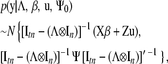
Therefore,

(8)

where Ψ=Ψ₀⊗I_n.

Recovering recursive causal structures:

As stated, most quantitative genetics applications of SEMs so far have used prespecified causal structures. An alternative is to implement algorithms that search for a causal structure. This section describes an algorithm that performs such a search for the model y_i=Λy_i+e_i. The application of the algorithm in the context of a mixed model is presented in the next section.

A recursive causal structure is represented by a directed acyclic graph (DAG), which is a set of variables connected by directed edges (arrows) representing direct causal relationships. A path in the causal structure is a sequence of connected variables, regardless of the direction of the arrows that connect them. Unconditionally, paths allow flows of dependence between variables in their extremes, unless there is a collider (variable with arrows pointing at them from opposite directions, like c in a → c ← b) in the path. Colliders block the flow of dependency in a path, which makes a and b independent in the structure above. Conditioning on a variable that is not in the extremes of the path blocks the flow of dependency if this variable is a noncollider (e.g., conditioning on c in a → c → b, a ← c ← b, or a ← c → b makes a and b independent) or allows the flow of dependency if this variable is a collider. Considering two variables a and b in a DAG, they are said to be d-separated conditionally on a subset S of variables if there are no paths that allow flows of dependency between a and b (i.e., no paths between a and b in a DAG such that all the colliders or its descendants are in S and no noncolliders are in S). Under some assumptions (which are discussed later), d-separations in the causal structure are reflected as conditional independencies in the joint probability distribution of the data. This can be explored to recover a causal structure or a class of equivalent causal structures (causal structures that result in joint probability distributions with the same conditional independence relationships) from the joint distribution of the data (Pearl 2000; Spirtes et al. 2000).

The IC algorithm (Verma and Pearl 1990; Pearl 2000) can be used to recover an underlying DAG structure (or a class of observationally equivalent structures) from observed associations between traits. The search is based on queries about conditional independencies between variables and on the assumption that such independencies reflect d-separations in the underlying DAG. The input of the algorithm is a correlation matrix between observable variables, from which marginal and conditional dependencies can be evaluated. The output is a partially oriented graph representing a class of equivalent causal structures, which generally results in an important constraint on the initial causal hypothesis space that could be used to fit the SEM. Partially oriented graphs are graphs with directed and undirected edges. The latter represent symmetric direct relationships between pairs of variables, since they do not specify direction of causal relationship.

Considering a set V of random variables, the IC algorithm can be described by the following steps:

1. For each pair of variables a and b in V, search for a set of variables S_ab such that a is independent of b given S_ab. If a and b are dependent for every possible conditioning set, connect a and b with an undirected edge. This step results in an undirected graph U. Connected variables in U are called adjacent.

2. For each pair of nonadjacent variables a and b with a common adjacent variable c in U (i.e., a–c–b), search for a set that contains c such that a is independent of b given . If this set does not exist, then add arrowheads pointing at c (a → c ← b). If this set exists, then continue.

3. In the resulting partially oriented graph, orient as many undirected edges as possible in such a way that it does not result in new colliders or in cycles.

The goal of the first step of the algorithm is to obtain a graph that specifies pairs of traits that are directly connected by an edge, but without specifying causal direction. Adjacent variables of an undirected graph are not d-separated, regardless of the conditioning set of variables. Therefore, adjacent variables are not probabilistically independent given any possible set of variables.

The aim of the second step is to orient edges by searching for variables in the undirected graph where the causal paths collide. Structures where a collider is directly caused by two nonadjacent variables are called unshielded colliders (Spirtes et al. 2000). In the unshielded collider a → c ← b, variables a and b are called parents of c, and the latter is called child of a and b. Nonadjacent parents of a collider variable are d-separated given at least one set of variables, but not if conditioned to any set of variables that contains the collider. The observational consequence of this is the probabilistic dependence between the nonadjacent parents conditionally on every possible set of variables that contains the common child.

The third step is to perform every further edge orienting that does not result in a new collider or in a cycle. As an example, consider that three variables in a hypothetical graph resulting from step 2 are connected as a → b – c. After step 2, the edge between b and c must be oriented toward c. The opposite direction would result in an additional collider. Similar edge orienting is performed if any of the possible directions results in a cycle. Background knowledge or prior beliefs can be incorporated into the search algorithm, further constraining the output by either forbidding or coercing the existence of an edge or by performing additional edge orienting (Spirtes et al. 2000; Shipley 2002).

The search performed by the IC algorithm relies on the connection between causal graphs and the probability distributions that they generate. This connection is established on the basis of the assumption that there are no hidden variables that affect more than one of the variables considered in the search (i.e., causal sufficiency assumption). If this assumption does not hold, the connection between d-separations and conditional independencies may be lost. Take as an example one set of observed variables O and two variables a and b that are not connected by an edge in the underlying causal structure. If a and b have a common hidden cause, they are expected to be conditionally dependent given every possible set of variables in O. This would result in including a misleading edge between a and b in the partially oriented graph selected by the IC algorithm.

In the SEM presented in (1), residuals e_i account for the effects of the remaining unknown causes of the phenotypic traits considered. The assumption of causal sufficiency implies that the search should be performed on a set of variables that includes every common cause of two or more of these variables. Therefore, under this assumption, residuals in SEMs are constructed as independent, which has been an assumption in recent applications of such models to quantitative genetics (De los Campos et al. 2006a; De Maturana et al. 2009; Heringstad et al. 2009).

The queries of the IC algorithm require pairs of variables to be declared as conditionally dependent or conditionally independent. The decision is based on partial correlations estimated from a sample. Therefore, the uncertainty about the partial correlations should be accounted for in the decision required. In a frequentist approach, these statistical decisions may be done by testing the null hypothesis of a vanishing partial correlation. In a Bayesian approach, these decisions can be made using highest posterior density intervals for the partial correlations.

Causal structure search within a mixed models context:

In the formulation described in the previous section, model residuals are regarded as independent, and recursive effects are used to model (interpret) patterns of covariability between observable variables. However, in mixed models, the patterns of covariability between phenotypes may be due either to causal links between traits or to genetic reasons. In other words, correlated random genetic effects can act as confounders if one tries to select a causal structure on the basis of the joint distribution of the phenotypes, even if residuals are assumed as independent.

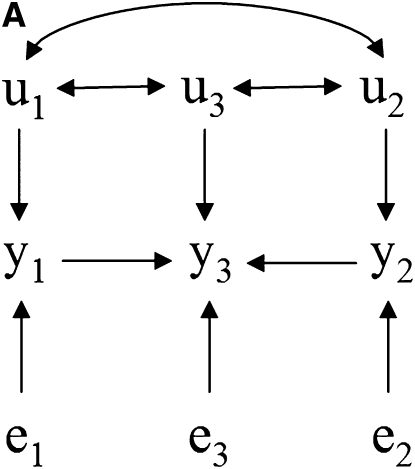
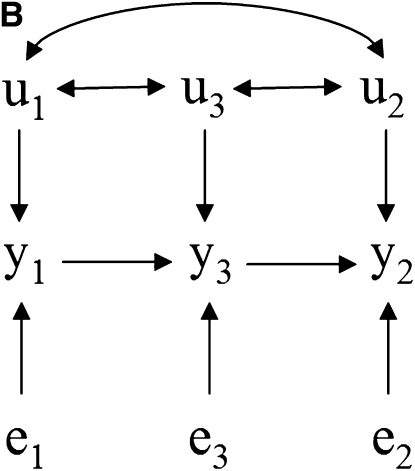
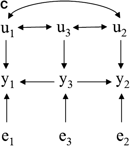
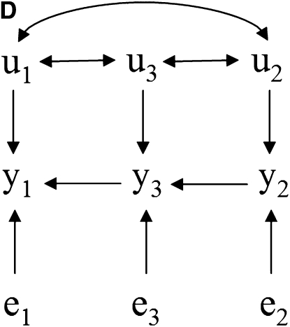
Take as an example the scenarios depicted in Figure 1, where there are recursive relationships among phenotypes y₁, y₂, and y₃, with uncorrelated residuals (e₁, e₂, and e₃) and correlated additive genetic effects (u₁, u₂, and u₃). The connection between the causal structure among phenotypes and their joint probability distribution does not hold in a model where genetic effects are uncontrolled hidden variables. In this case, y₁ and y₂ are not marginally independent in Figure 1A because of the covariance between u₁ and u₂. For the same reason, they are not independent given the phenotype y₃ in Figure 1, B–D.

Figure 1.—

(A–D) Causal structures for three observed variables (y₁, y₂, and y₃), with independent residuals (e₁, e₂, and e₃) and correlated additive genetic effects (u₁, u₂, and u₃). Unobservable genetic effects act as confounders if not considered in the model, and the joint distribution of observed variables would not represent properly the expected conditional independencies based on the causal structure among traits.

Nonetheless, additive relationships between individuals give a mean for “controlling” for this confounder. This can be done, for example, if there is pedigree or marker information on subjects. In this approach, d-separations are reflected as conditional independencies on the distribution of phenotypes after taking into account the additive genetic effects (i.e., the distribution of the phenotypes conditionally on the genetic effects). In Figure 1A, y₁ and y₂ are independent given the additive genetic effects. In Figures 1, B–D, the same observed variables are independent given the additive genetic effects and phenotype y₃. A SEM that accounts for additive genetic effects can be written as (2), which implies that

Note that (I_t−Λ)⁻¹G₀(I_t−Λ)′⁻¹ and (I_t−Λ)⁻¹Ψ₀(I_t−Λ)′⁻¹ are the covariance matrices of additive genetic effects (G₀^*) and of residuals (R₀^*) obtained from a standard multiple-trait mixed model that accounts for covariance between genetic effects and residuals from different traits, but not for causal relationships between phenotypes (Gianola and Sorensen 2004; Varona et al. 2007). The covariance matrix of y_i can be rewritten as Var (y_i) = G₀*+R₀*, and the covariance matrix between traits conditionally on the additive genetic effects can be represented as Var(y_i|u_i)=(I_t−Λ)⁻¹Ψ₀(I_t−Λ)′⁻¹=R₀*. Therefore, estimates of R₀* can be used to select a causal structure among phenotypes. This (co)variance matrix can be inferred using frequentist or Bayesian methods. In a Bayesian framework one draws samples from the posterior distribution of R₀* and these samples are used to obtain measures of uncertainty about this matrix, while accounting for uncertainty of all other parameters included in the reduced MTM. Next, we describe how to search for a causal structure in a mixed models context, using samples from the posterior distribution of R₀* as input to the IC algorithm:

1. Fit a MTM and draw samples from the posterior distribution of R₀*.

2. Apply the IC algorithm to the posterior samples of R₀* to make the statistical decisions required. Specifically, for each query about the statistical independence between variables a and b given a set of variables S and, implicitly, the genetic effects, do the following:

   1. Obtain the posterior distribution of residual partial correlation ρ_a,b|S. These partial correlations are functions of R₀*. Therefore their posterior distribution can be obtained by computing the correlation at each sample drawn from the posterior distribution of R₀*.
   2. Compute the 95% highest posterior density (HPD) interval for the posterior distribution of ρ_a,b|S.
   3. If the HPD interval contains 0, declare ρ_a,b|S as null. Otherwise, declare a and b as conditionally dependent.

3. Fit a SEM using the selected causal structure (or one member within the class of observationally equivalent structures retrieved by the IC algorithm) as a “TRUE” causal structure.

EXAMPLE

This section illustrates concepts described previously by applying the proposed methodology to simulated data. The data generating process and the models used for inferences are described first, and results are presented and discussed subsequently. The analysis was carried out using programs written in R (R Development Core Team 2008), which are available from the authors upon request.

Data generating process:

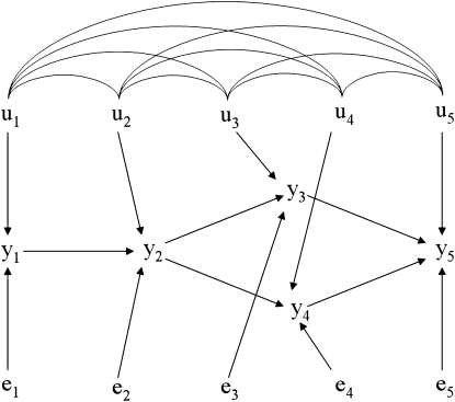
Observations for 1800 subjects were generated from a recursive model involving five traits based on the acyclic causal structure considered by Shipley (1997) (Figure 2), with independent residuals. In addition, it was assumed that the observed variables were affected by a system of correlated additive genetic effects simulated for 300 inbred lines, with 6 individuals observed per line.

Figure 2.—

Diagram of the model from which simulated data were drawn; y_j is an observed measurement on trait j, u_j is the additive genetic effect contributing to trait j, and e_j is a model residual associated with trait j. Arcs connecting u's represents genetic correlations. The causal structure is adapted from Shipley (1997).

The SEM from which data were generated can be represented as

where y_ijk and e_ijk are the phenotype and residual effects for trait j (j = 1, … , 5) observed on the ith individual belonging to the kth inbred line, μ_j is the mean value of trait j, u_jk is the additive genetic effect of inbred line k for trait j, and λ_jj′ is the rate of change of trait j with respect to trait j′.

Additive genetic effects assigned for the 300 inbred lines were simulated as 50 unrelated clusters of 6 lines derived from full-sib individuals. Therefore, the genetic relationship matrix (A) between lines was a block diagonal matrix in which each block consisted of a 6 × 6 matrix where the off-diagonal entries were 0.5 (additive relationship between full sibs) and the diagonal entries were 1. Vectors of additive genetic effects and residuals were sampled from u ∼ N(0, G₀⊗A) and e ∼ N(0, Ψ₀⊗I_n), respectively.

Parameters used in the simulation were arbitrarily chosen as

Inferences:

Inference was based on a SEM with independent residuals as given by Ψ₀. A fully recursive SEM, where every entry below the main diagonal of Λ is a free parameter, was used to obtain the posterior distribution of R₀*. Furthermore, a SEM was fit using the selected causal structure. The following joint prior distribution was assumed for location and dispersion parameters of model (7),

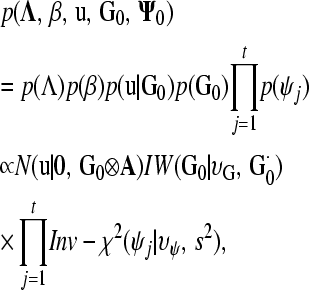where N(u|0, G₀⊗A) is a multivariate normal density centered at 0 with covariance matrix G₀⊗A, IW(G₀|υ_G, G₀^·) is an inverse Wishart density with υ_G d.f. and scale matrix G₀^·, Inv-χ²(ψ_j|υ_ψ, s²) is a scaled inverse chi-square distribution with υ_ψ d.f. and scale s², and ψ_j is the variance of model residuals for trait j. Unbounded uniform distributions were assigned to each entry of Λ considered as a free parameter and to β. Finally, υ_G, G₀^·, υ_ψ, and s² were regarded as known hyperparameters of the prior distributions.

The joint posterior distribution of all unknowns in the model is then

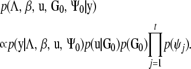The resulting distribution does not have a closed form, so a Gibbs sampler algorithm (Geman and Geman 1984) was employed for drawing samples from it, using fully conditional distributions. The derivations use standard results from Bayesian linear models (e.g., Sorensen and Gianola 2002; Gianola and Sorensen 2004).

A single chain of 40,000 iterations was run for each model. The initial 4000 iterations of each chain were discarded as burn-in, which was conservative relative to the 312 burn-in iterations indicated by the method of Raftery and Lewis (1992) implemented in the R BOA package (Smith 2007). The remaining 36,000 iterations were regarded as samples from the posterior distributions of the parameters.

Fully recursive model:

To select a causal structure to be used in a SEM, an unstructured residual covariance matrix inferred by fitting a standard multiple-trait model to the data was used to search for patterns of conditional independence that guide the selection of a class of equivalent causal structures. To estimate such a matrix, the data were analyzed using a fully recursive model, with an unstructured additive genetic covariance matrix and a diagonal residual covariance matrix. This model and the standard multiple-trait model have equivalent likelihoods (Varona et al. 2007), such that both models produce similar residual covariance matrices under different parameterizations. Therefore, the posterior distribution of an unstructured residual covariance matrix for a standard multiple-trait model can be obtained by fitting a fully recursive model and then transforming the estimated parameters in each iteration. The fully recursive model was reparameterized as

with

where Λ_fr is a matrix containing structural coefficients of a fully recursive model, R₀^* is an unstructured residual covariance matrix (i.e., that of a classical multiple-trait model), and Ψ_fr is the diagonal residual covariance matrix pertaining to the fully recursive model.

The following hyperparameter values were used for fitting the fully recursive model: s_fr² = 50 and υ_Ψfr = 3 for every entry of diagonal of Ψ_fr, υ_G = 7, and

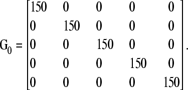Inferring causal structure:

The posterior distribution of R₀^* was used to select a recursive causal structure among phenotypes, via the IC algorithm. A partial correlation was considered as null if its 95% HPD interval contained 0. The partial correlation between traits a and b, conditional on a set of traits S, is represented as ρ_ab|S. The partial correlations are conditional not only on phenotypes in S but also on additive genetic effects, which are omitted in the notation subsequently.

Structural equation model under the selected causal structure:

On the basis of the chosen causal structure from the partially oriented graph retrieved by the IC algorithm, appropriate entries of Λ were treated as unknown for fitting the corresponding SEM using simulated data. Hyperparameter values used for the prior distributions of the dispersion parameters were those used for fitting the fully recursive model.

Results:

The posterior mean of matrix R₀*, obtained by transforming Ψ_fr, was

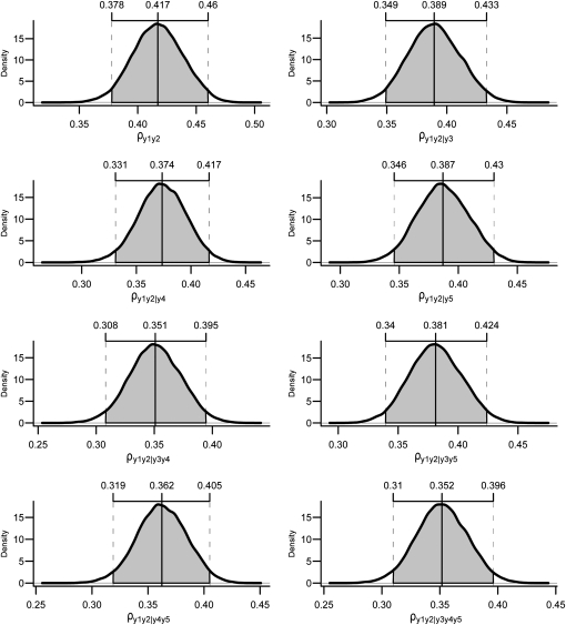
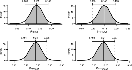
Applying the first step of the IC algorithm to samples from the posterior distribution of R₀* resulted in the undirected graph depicted in Figure 3A. Pairs of variables connected by edges had nonnull partial correlations regardless of the conditioning set (as illustrated in Figure 4 for pair [y₁, y₂] and in supporting information, Figure S1, Figure S2, Figure S3, and Figure S4 for the remaining pairs), where the HPD of the parameters did not contain 0. On the other hand, null partial correlations were found for the remaining pairs, as shown in Figure 5.

Figure 3.—

Undirected acyclic graph (A) resulting from step 1 of the IC algorithm and partially oriented graph (B) retrieved by the IC algorithm. Prior beliefs on the direction of the edge between y₁ and y₂ (pointing toward y₂) lead to the choice of structure (C) from the class of structures represented by B.

Figure 4.—

Posterior distributions and HPD intervals of total and partial correlations between y₁ and y₂, conditioned on every possible set of the remaining variables. The absence of null partial correlations leads the first step of the IC algorithm to insert an edge between y₁ and y₂.

Figure 5.—

Posterior distributions and HPD intervals of null partial correlations that prompt the IC algorithm to remove edges between the pairs of variables [y₁, y₃], [y₁, y₄], [y₁, y₅], [y₂, y₅], and [y₃, y₄].

The second step of the IC algorithm resulted in the partially oriented graph presented in Figure 3B. The sets of three variables formed by pairs of disconnected variables with one common adjacent variable in the undirected graph retrieved from the first step were y₁–y₂–y₃, y₁–y₂–y₄, y₃–y₂–y₄, y₂–y₃–y₅, y₂–y₄–y₅, and y₃–y₅–y₄. All of them were declared as noncolliders by the algorithm, except for y₃–y₅–y₄. The algorithm directed both edges toward y₅ because y₃ and y₄ did not present null partial correlation when y₅ was in the conditioning set of variables, as shown in Figure 6.

Figure 6.—

Posterior distributions and HPD intervals of partial correlations between y₃ and y₄ given every possible set of remaining variables containing y₅. The absence of null partial correlations prompted the IC algorithm to declare the path y₃–y₅–y₄ as an unshielded collider, as presented in Figure 3B.

The third step of the IC algorithm did not change the partially oriented graph retrieved from the second step, since there was no further edge orienting to be performed only on the basis of the residual distribution.

The output of the IC algorithm is a partially oriented acyclic graph that represents a class of equivalent structures, each of which is capable of producing the pattern of conditional independencies resulting from R₀*. The true causal structure is an instance of the selected class, which contains only four alternative structures (Shipley 2002). However, information such as time precedence or other sources of prior knowledge may be used for further edge orienting. Take the pair [y₁, y₂] as an example. The existence of an edge between this pair is recognized by the IC algorithm, independently of any sort of prior knowledge, since the correlation between them is not declared as null regardless of the conditional set of remaining variables (Figure 4). However, the algorithm is not able to recognize the direction of this edge, since the pair is not part of an unshielded collider and, in the structure retrieved by the second step of the algorithm, it could be directed in either way without creating new colliders or cycles in the graph. However, if one knows, for example, that y₁ precedes y₂ in time, this prior knowledge is not sufficient to impose or forbid an edge between them, but it is sufficient to orient an edge already detected by the algorithm. If, say, this information is used to point the arrowhead of this edge toward y₂, all remaining edges would be oriented as in Figure 3C. Given y₁ → y₂, edges y₂–y₃ and y₂–y₄ should be oriented toward y₃ and y₄, respectively (Shipley 2002). Any other configuration would result in colliders in y₂, representing a causal structure that is not compatible with R₀*.

Table S1 presents the posterior means and 95% HPD intervals of dispersion parameters and structural coefficients, obtained from a SEM fit conditionally on the causal structure chosen. Input parameter values used to simulate the data were within the aforementioned HPD intervals, with the genetic covariance between traits 2 and 5 being the exception. As additional examples, the proposed approach was used to study data simulated from two models based on different directed acyclic graphs. The results obtained from these analyses are displayed in File S1, Figure S5, and Figure S6.

DISCUSSION

The work by Gianola and Sorensen (2004) prompted interest in SEMs for analysis of quantitative traits. The authors noted the huge number of possible causal structures, even in studies with only a few traits. Wu et al. (2007) stated that prior knowledge could be used to reduce the number of causal structures under consideration, and this is what has been done in most of the applications of SEMs in animal breeding. However, this strategy is only as good as the preexistent theory leading to the prior knowledge (Shipley 2002). Typically, prior beliefs are used to choose one structure or a small set of structures. When a set of structures is chosen, adjusted models may be compared on the basis of criteria such as AIC or BIC. However, the causal structures of the models compared are part of a small subset of all possible structures, so that there may be other models that fit as well or even better than the preselected ones. One could propose an exhaustive search based on a model comparison criterion, which would require adjustment of models containing each possible causal structure. In most situations there are a huge number of possible causal structures (according to Shipley 1997, there are ∼59,000 possible acyclic causal structures involving only five traits), which makes this approach not feasible.

Using the IC algorithm improves upon the current approach by exploring the causal structure space without relying only on prior causal knowledge. The algorithm searches for a class of equivalent acyclic causal structures compatible with the observed patterns of conditional independencies among traits. This search is not based on the aforementioned model selection criteria, although the selected structures are expected to result in better scores for these criteria as well. This is because it returns structures that better adjust to a given pattern of conditional independencies and that are minimal; i.e., they result in SEMs with less expressive power or less flexibility when adjusting to a covariance matrix (Pearl 2000). Prior beliefs may still be used to choose the more appealing structures from the structure class selected. Depending on the context, the algorithm may be modified in such a way that prior knowledge overrides the standard algorithm's output, coercing or forbidding an edge or a direction of arrowheads to exist in the causal structure (Spirtes et al. 2000).

The assumptions of the IC algorithm are not stronger than assumptions considered in recent application of SEMs in quantitative genetics. In these applications, not only covariance matrices of random variables were assumed to be structured (usually diagonal), but also the causal structure itself was assumed to be known. Here we impose a diagonal residual covariance matrix in the SEM, as in De los Campos et al. (2006a), De Maturana et al. (2009), and Heringstad et al. (2009). Within this construction, a causal structure that is compatible with the joint probability distribution of the data is searched.

However, the IC algorithm cannot be applied directly to the joint distribution of the phenotypes, because genetic effects may act as confounders. For the simulated data, applying the search algorithm on the unconditional covariance matrix of the phenotypes resulted in an incorrect output for step 1: besides the undirected edges recognized in the example described, the pairs of traits [y₂, y₅] and [y₁, y₅] were connected by edges as well. An additional mistake was declaring the path y₃–y₂–y₄ as an unshielded collider (y₃ → y₂ ← y₄) in step 2. A main contribution of this article was to propose a methodology of search for causal structures in the context of mixed models applied to quantitative genetics. The methodology proposed exploits the fact that it is possible to obtain the distribution of the phenotypes conditional to the genetic confounders by controlling the genetic effects. This is done by fitting a MTM, which accounts for such genetic effects.

In the example described here, all statistical decisions were correct and, consequently, all d-separations were correctly detected. The problem becomes more challenging as causal relationships are weaker. After performing a similar simulation but with all structural coefficients reduced in absolute value by 50% (results not shown), the same undirected graph was retrieved by the first step of the algorithm. However, the second step failed to recognize the unshielded collider y₃ → y₅ ← y₄, as the HPD interval of was [−0.003, 0.098]. As a consequence, y₅ was declared incorrectly as a noncollider. As one would expect, statistical decisions are poorer as the posterior distribution of the partial correlations gets less sharp (e.g., smaller data sets or underidentifiability of model parameters). Less informative scenarios may lead to a larger probability of incorrectly missing direct connections or adding incorrect edges, besides incorrectly missing or adding arrowheads. After using the proposed approach on data simulated as described in the Data generating process section, but with a single subject for each one of the 300 “inbred line effects,” the output was the same as that obtained when all structural coefficients were reduced in absolute value by 50%. However, the expected output was obtained when two or more subjects were simulated for each inbred line.

In these scenarios that lead to less sharp posterior distributions of the partial correlations, if statistical decisions made by the IC algorithm are based on HPD intervals of high content (which coupled with higher parameter uncertainty leads to large intervals), the algorithm looses efficiency in detecting weaker partial correlations. Since there is no preference between protecting from failure to detect nonnull partial correlations and declaring true null partial correlations as nonnull, it would seem sensible to decrease the probability content of the HPD intervals used for decisions when the posterior distributions of partial correlations are less sharp (Shipley 2002). Nevertheless, errors in the statistical decisions do not necessarily cause mistakes in the inference. For example, if there is more than one conditioning set that d-separates two variables and some, but not all of them, mirror a vanishing partial correlation in the sample analyzed, the resulting undirected graph would be the same, because the edges are discarded in the presence of at least one null partial correlation (Spirtes et al. 2000).

Genetic effects (and their correlations) enter into both the reduced MTM and the recursive SEM. However, parametric interpretations differ according to the model used. As an example, consider the additive genetic correlation between hypothetical traits a and b, and let a cause b. Under a recursive model, the additive genetic correlation accounts for a linear association between two unobservable variables, each directly affecting a specific trait. However, this would not be the sole source of genetic correlation between these traits under a model that does not account for recursiveness, because there is an indirect association between the additive genetic effect of a and phenotype b, mediated by phenotype a. Under the recursive model, the genetic correlation does not account for this indirect effect. On the other hand, the additive genetic correlation under a MTM accounts for all association effects, irrespective of whether these effects are direct or otherwise in a recursive context. Because of this, the additive genetic correlation under a MTM could be different from 0 even if genetic additive effects are uncorrelated in the recursive context (Gianola and Sorensen 2004). Genetic correlations that are not mediated by causal relationships among phenotypes are confounders that do not allow a search for causal structures from phenotypic information alone. The present study proposed a search for causal structures in the covariance matrix of y after effects of such confounders are taken into account.

Controlling for additive genetic covariances restores the connection between the joint distribution of phenotypes and causal structure. In cases where other important random effects may act as additional confounders, such as maternal effects, R₀* should be inferred from mixed models that account for these effects as well. Furthermore, models that do not account fully for additive genetic confounder effects could lead to misleading results. For example, in a sire model, genetic effects inherited from the sire are taken into account, whereas genetic effects inherited from the dam are omitted in the model. Maternally inherited alleles, however, will be a source of covariance between phenotypes, and their effects would contribute to the residual covariance structure. Hence, the sire model will fail to remove the effect of additive genetic confounders.

The computation requirements of the proposed approach increase as the set of analyzed traits gets larger. For the example presented in this article, 10 pairs of traits are analyzed in step 1 of the IC algorithm ([y₁, y₂], [y₁, y₃], [y₁, y₄], [y₁, y₅], [y₂, y₃], [y₂, y₄], [y₂, y₅], [y₃, y₄], [y₃, y₅], and [y₄, y₅]). For each pair, dependence was evaluated conditionally on 8 different subsets of the remaining traits, as illustrated for [y₁, y₂] in Figure 4. If a set of 4 traits is analyzed, dependencies relative to 6 pairs of variables should be assessed in the first step, each one conditionally on 4 different subsets. In a case with 6 traits, dependencies on 15 pairs of variables need to be evaluated in the first step, each one conditionally on 16 different subsets. Furthermore, increasing the number of traits or the size of the data set also increases computational time to fit the fully recursive model. The length of the Monte Carlo chain containing posterior samples of the residual covariance matrix also affects computational time of the proposed approach. This takes place not only because of the increased time required to sample the chain, but also because partial correlations must be calculated from each sample of the covariance matrix to obtain their posterior distribution. The described analysis was performed in a Dell Precision T7400 workstation, with 16 Gb memory and CPU 64-bit dual-core Intel Xeon processors, running on Red Hat Enterprise Linux. It took ∼6 hr to obtain the posterior samples for the parameters of the fully recursive model and ∼15 min to obtain a list of selected partially oriented graph's edges and unshielded colliders from the posterior samples of the MTM residual covariance matrix.

Models that describe only the probabilistic relationship between traits are insufficient for predicting effects of interventions, while causal models may be used to infer how probabilities would change as a result of external interventions (Pearl 2000). The concepts described in this study apply beyond quantitative genetics. For example, the techniques for searching causal structures could be used for predicting the effect of farm management or veterinary decisions in which genetic covariances act as confounders.

References

- Akaike, H., 1973. Information theory and an extension of the maximum likelihood principle, pp. 267–291 in 2nd International Symposium on Information Theory, edited by B. N. Petrov and F. Csaki. Publishing House of the Hungarian Academy of Sciences, Budapest.
- Aten, J. E., T. F. Fuller, A. J. Lusis and S. Horvath, 2008. Using genetic markers to orient the edges in quantitative trait networks: the NEO software. BMC Syst. Biol. 2 34. [DOI] [PMC free article] [PubMed] [Google Scholar]
- Chaibub Neto, E., T. C. Ferrara, A. D. Attie and B. S. Yandell, 2008. Inferring causal phenotype networks from segregating populations. Genetics 179 1089–1100. [DOI] [PMC free article] [PubMed] [Google Scholar]
- Chen, L. S., F. Emmert-Streib and J. D. Storey, 2007. Harnessing naturally randomized transcription to infer regulatory relationships among genes. Genome Biol. 8 R219. [DOI] [PMC free article] [PubMed] [Google Scholar]
- De los Campos, G., D. Gianola, P. Boettcher and P. Moroni, 2006. a A structural equation model for describing relationships between somatic cell score and milk yield in dairy goats. J. Anim. Sci. 84 2934–2941. [DOI] [PubMed] [Google Scholar]
- De los Campos, G., D. Gianola and B. Heringstad, 2006. b A structural equation model for describing relationships between somatic cell score and milk yield in first-lactation dairy cows. J. Dairy Sci. 89 4445–4455. [DOI] [PubMed] [Google Scholar]
- De Maturana, E. L., X. L. Wu, D. Gianola, K. A. Weigel and G. J. M. Rosa, 2009. Exploring biological relationships between calving traits in primiparous cattle with a Bayesian recursive model. Genetics 181 277–287. [DOI] [PMC free article] [PubMed] [Google Scholar]
- Geman, S., and D. Geman, 1984. Stochastic relaxation, Gibbs distributions and Bayesian restoration of images. IEEE Trans. Patt. Anal. Mach. Intell. 6 721–741. [DOI] [PubMed] [Google Scholar]
- Gianola, D., and D. Sorensen, 2004. Quantitative genetic models for describing simultaneous and recursive relationships between phenotypes. Genetics 167 1407–1424. [DOI] [PMC free article] [PubMed] [Google Scholar]
- Haavelmo, T., 1943. The statistical implications of a system of simultaneous equations. Econometrica 11 1–12. [Google Scholar]
- Heringstad, B., X.-L. Wu and D. Gianola, 2009. Inferring relationships between health and fertility in Norwegian red cows using recursive models. J. Dairy Sci. 92 1778–1784. [DOI] [PubMed] [Google Scholar]
- Konig, S., X. L. Wu, D. Gianola, B. Heringstad and H. Simianer, 2008. Exploration of relationships between claw disorders and milk yield in Holstein cows via recursive linear and threshold models. J. Dairy Sci. 91 395–406. [DOI] [PubMed] [Google Scholar]
- Li, R., S. W. Tsaih, K. Shockley, I. M. Stylianou, J. Wergedal et al., 2006. Structural model analysis of multiple quantitative traits. PLoS Genet. 2 e114. [DOI] [PMC free article] [PubMed] [Google Scholar]
- Liu, B., A. De La Fuente and I. Hoeschele, 2008. Gene network inference via structural equation modeling in genetical genomics experiments. Genetics 178 1763–1776. [DOI] [PMC free article] [PubMed] [Google Scholar]
- Pearl, J., 1988. Probabilistic Reasoning in Intelligent Systems: Networks of Plausible Inference. Morgan Kauffman, San Mateo, CA.
- Pearl, J., 2000. Causality: Models, Reasoning and Inference. Cambridge University Press, Cambridge, UK.
- R Development Core Team, 2008. R: A Language and Environment for Statistical Computing. R Foundation for Statistical Computing, Vienna. http://www.R-project.org.
- Raftery, A. E., and S. Lewis, 1992. How many iterations in the Gibbs sampler? pp. 763–773 in Bayesian Statistics IV, edited by J. M. Bernardo, J. Berger, A. P. Dawid and A. F. M. Smith. Oxford University Press, Oxford.
- Schadt, E. E., J. Lamb, X. Yang, J. Zhu, S. Edwards et al., 2005. An integrative genomics approach to infer causal associations between gene expression and disease. Nat. Genet. 37 710–717. [DOI] [PMC free article] [PubMed] [Google Scholar]
- Schwarz, G., 1978. Estimating the dimension of a model. Ann. Stat. 6 461–464. [Google Scholar]
- Shipley, B., 1997. Exploratory path analysis with applications in ecology and evolution. Am. Nat. 149 1113–1138. [DOI] [PubMed] [Google Scholar]
- Shipley, B., 2002. Cause and Correlation in Biology. Cambridge University Press, Cambridge, UK/London/New York.
- Smith, B. J., 2007. BOA: an R package for MCMC output convergence assessment and posterior inference. J. Stat. Softw. 21 1–37. [Google Scholar]
- Sorensen, D., and D. Gianola, 2002. Likelihood, Bayesian and MCMC Methods in Quantitative Genetics. Springer-Verlag, New York.
- Spirtes, P., C. Glymour and R. Scheines, 2000. Causation, Prediction and Search, Ed. 2. MIT Press, Cambridge, MA.
- Varona, L., D. Sorensen and R. Thompson, 2007. Analysis of litter size and average litter weight in pigs using a recursive model. Genetics 177 1791–1799. [DOI] [PMC free article] [PubMed] [Google Scholar]
- Verma, T., and J. Pearl, 1990. Equivalence and synthesis of causal models. Proceedings of the 6th Conference on Uncertainty in Artificial Intelligence, Cambridge, MA, pp. 220–227. Elsevier, Amsterdam.
- Wright, S., 1921. Correlation and causation. J. Agric. Res. 201 557–585. [Google Scholar]
- Wu, X.-L., B. Heringstad, Y. M. Chang, G. De los Campos and D. Gianola, 2007. Inferring relationships between somatic cell score and milk yield using simultaneous and recursive models. J. Dairy Sci. 90 3508–3521. [DOI] [PubMed] [Google Scholar]
- Wu, X.-L., B. Heringstad and D. Gianola, 2010. Bayesian structural equation models for inferring relationships between phenotypes: a review of methodology, identifiability, and applications. J. Anim. Breed. Genet. 127 3–15. [DOI] [PubMed] [Google Scholar]