

Abstract
Motivation: A global map of transcription factor binding sites (TFBSs) is critical to understanding gene regulation and genome function. DNaseI digestion of chromatin coupled with massively parallel sequencing (digital genomic footprinting) enables the identification of protein-binding footprints with high resolution on a genome-wide scale. However, accurately inferring the locations of these footprints remains a challenging computational problem.
Results: We present a dynamic Bayesian network-based approach for the identification and assignment of statistical confidence estimates to protein-binding footprints from digital genomic footprinting data. The method, DBFP, allows footprints to be identified in a probabilistic framework and outperforms our previously described algorithm in terms of precision at a fixed recall. Applied to a digital footprinting data set from Saccharomyces cerevisiae, DBFP identifies 4679 statistically significant footprints within intergenic regions. These footprints are mainly located near transcription start sites and are strongly enriched for known TFBSs. Footprints containing no known motif are preferentially located proximal to other footprints, consistent with cooperative binding of these footprints. DBFP also identifies a set of statistically significant footprints in the yeast coding regions. Many of these footprints coincide with the boundaries of antisense transcripts, and the most significant footprints are enriched for binding sites of the chromatin-associated factors Abf1 and Rap1.
Contact: jay.hesselberth@ucdenver.edu; william-noble@u.washington.edu
Supplementary information: Supplementary material is available at Bioinformatics online.
1 INTRODUCTION
The production of a genome-wide cis-regulatory map, indicating where transcription factors (TFs) bind genomic DNA to regulate gene expression, is critical to understanding gene regulation and genome function. Many experimental methods, such as gel-shift assays and promoter mutation analysis, can be used to identify transcription factor binding sites (TFBSs), but these low-throughput methods are time-consuming and thus difficult to apply to whole genomes. Recently, high-throughput biological techniques have been used to detect binding sites. For example, chromatin immunoprecipitation can be combined with either DNA microarrays (ChIP-Chip; Ren et al., 2000) or massively parallel DNA sequencing (ChIP-Seq; (Johnson et al., 2007) to identify DNA regions bound by a specific TF. However, these ChIP-based approaches require TF-specific antibodies or epitope-tagged constructs to precipitate TFs and their associated DNA sequences.
A recently described, complementary method, known as digital genomic footprinting, provides a genome-wide profile of DNA accessibility at nucleotide resolution (Hesselberth et al., 2009). The method relies upon well-developed chromatin profiling techniques that have been used extensively to detect regulatory regions in vivo (Dorschner et al., 2004). Because TFs displace canonical nucleosomes in chromatin, their binding to regulatory regions leads to high sensitivity to cleavage by the endonuclease DNaseI; thus, DNaseI hypersensitive sites are enriched for active regulatory elements (Wu, 1980). Digital genomic footprinting is essentially DNaseI digestion coupled with massively parallel sequencing. Hesselberth et al. (2009) demonstrated that, when zooming into a hypersensitive site, nucleotides occupied by TFs show an under-representation of cleavage events relative to the neighboring nucleotides. Essentially, the footprint of the protein binding event can be visualized, as illustrated in Figure 1. Such data make it feasible to identify protein binding regions with high positional resolution on a genomic scale.
Fig. 1.
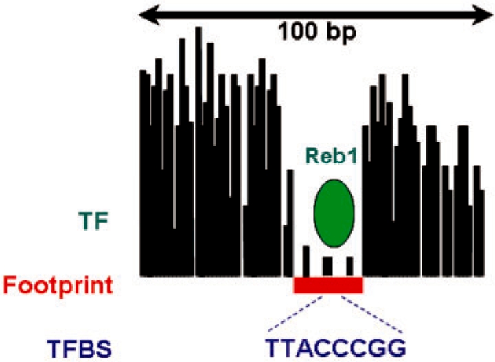
A protein-binding footprint, as produced by digital genomic footprinting. The height of each bar indicates the number of cleavage events observed at the corresponding nucleotide. The sequence TTACCCGG occurring within the footprint corresponds to the binding site of the TF Reb1.
Given DNaseI cleavage data at nucleotide resolution, the goal of our study is 2-fold. First, we describe a method for identifying protein-binding footprints. This task is analogous to existing methods for peak finding in ChIP-seq data (Johnson et al., 2007; Robertson et al., 2007; Valouev et al., 2008). These approaches first build profiles based on sequencing reads, and then identify peaks in the resulting profile. However, because of the difficulties in isolating a pure sample of TF-bound DNA fragments and because of the length variability of the TF-bound DNA fragments, ChIP-seq does not generally produce sufficient resolution to locate TFBSs precisely. The method that we describe, in constrast, is specifically designed to find small regions of low accessibility to DNaseI, corresponding to a single protein-binding event. Our second goal is to discover TFBSs in the predicted footprints, and to use the footprints to improve our understanding of yeast genome biology. Unlike ChIP-based assays, which target a single protein, digital genomic footprinting identifies binding events for any protein. Consequently, we must infer which protein corresponds to each observed footprint.
In this article, we present a dynamic Bayesian network (DBN)-based approach, called DBFP, to identify protein-binding footprints from digital footprinting data. DBNs are generalizations of both Bayesian networks (BNs) and hidden Markov models (HMMs) (Bilmes and Bartels, 2005), and they have been successfully applied to various computational biology problems (Klammer et al., 2008; Reynolds et al., 2008; Yao et al., 2008). Our previous study coupled depletion scoring with a greedy procedure to select non-overlapping regions that are depleted of DNaseI cleavage (Hesselberth et al., 2009). In this study, we use a DBN to replace the ad hoc greedy procedure, which allows footprints to be identified and missing data to be handled in a probabilistic framework. DBFP detects candidate footprints as regions of depleted cleavage relative to a local background and assigns a statistical confidence estimate to each candidate based on an empirical null model. Evaluated using gold-standard sets derived from a compendium of conserved protein-binding motifs (MacIsaac et al., 2006), DBFP outperforms our previously described algorithm in terms of precision achieved at a fixed recall.
Using DBFP, we assign a statistical confidence estimate to each identified footprint, yielding a collection of 4679 footprints from the yeast intergenic regions with an estimated false discovery rate (FDR) of 5%. We show that these footprints are preferentially located near transcription start sites (TSSs) and are strongly enriched for known TFBS. We also show that the remaining footprints that do not contain known binding sites are preferentially located close to other footprints, suggesting that some of the footprints may involve non-specific binding mediated by an adjacent sequence-specific binding event. Finally, we demonstrate that the digital genomic footprinting data also reveal potential binding events within coding regions. Many of the footprints detected within coding regions are preferentially located near the TSSs of previously identified antisense transcripts, and the most significant footprints are highly enriched for binding sites of the chromatin-associated TFs Abf1 and Rap1.
2 METHODS
By mapping high-throughput sequencing reads to a reference genome, following the strategy outlined by Hesselberth et al. (2009), we obtained a set of genomic locations of DNaseI cleavages, called tags. The tag count of a particular position indicates the number of tags occurring at that position. However, not every genomic position is assigned a tag count. Because the end sequencing proceeds in a strand-specific manner, sequencing reads are strand-specific. A genomic position can then be associated with two types of reads, one for each strand. A location is called uniquely mappable on one strand if the reads starting at the location on that particular strand cannot be mapped to any other location in the reference genome on either strand. In this work, we only consider uniquely mappable reads. Moreover, we assign tag counts only to positions that are uniquely mappable on both strands. Positions that are not uniquely mappable on both strands are considered missing data. In addition to tag counts and mappability information, the inputs to our method include two parameters that specify the size range of footprints to be identified, kmin and kmax. In this study, we search for footprints of 8–30 bp, which is usually the size of TFBSs.
Given the inputs described above, DBFP generates as output a list of non-overlapping footprints ranked by a statistical confidence score. We use the q-value (Storey and Tibshirani, 2003) to measure the statistical significance of footprints. The q-value of a footprint is defined as the minimal FDR threshold at which the footprint is deemed significant.
Our approach consists of three phases. First, we build a DBN to identify candidate footprint segments of width from kmin to kmax. Second, we compute a depletion score for every footprint segment. Finally, we repeat the entire procedure on the shuffled input data to generate a list of null scores. These null scores are used to estimate q-values. The approach is described in detail in the following sections.
2.1 A dynamic Baeyesian network for footprint detection
Given the genome-wide data of tag counts and mappability, we build a DBN for unsupervised segmentation of the genome into three types of non-overlapping regions as follows. Among these three types, footprint segments are our primary targets.
Footprint: this type of segment is depleted of tags and has low tag count variance. Each segment's width is constrained to lie between kmin and kmax, inclusive. Moreover, footprint segments are flanked on both sides by segments enriched in tags, because footprints correspond to regions of low accessibility in the midst of regions of high accessibility.
Background: similar to footprint segments, this type of segment has low tag counts and low tag count variance. However, background segments tend to be wide, with a width constraint > kmax.
Hypersensitive: this type of segment is enriched for tags and has relatively high tag count variance.
As an example, Figure 2a shows our network for two consecutive positions. The whole DBN actually extends over all genomic positions, and each position (except the first and last) is modeled by a copy of the same Bayesian network. The DBN is implemented using the Graphical Models ToolKit (GMTK; Bilmes and Zweig, 2002). The details of this network are described below.
Fig. 2.
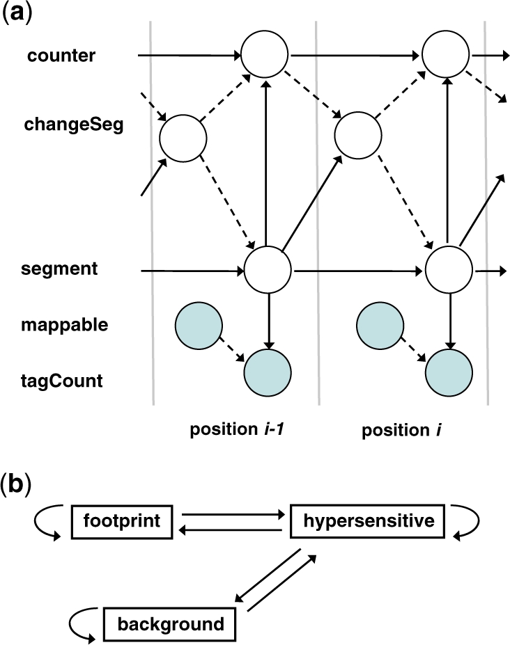
The DBN for footprint identification. (a) The network for two consecutive positions. Observed variables are represented by shadowed nodes. A dashed edge between two nodes indicates that the parent node is a switching parent. (b) The transition diagram of segment states. Note that no transition is allowed between the states footprint and background.
TagCount is an observed variable representing the number of tags that occur at each position. In order to reduce the variance of tag counts and the computational complexity of training and decoding, we discretize the original tag counts into 20 bins according to the genome-wide distribution. The bin boundaries are selected to make the bin counts as close to uniform as possible. The hidden variable segment has three states, indicating which segment type each position belongs to. These two variables form the backbone of the DBN, which is also a typical HMM. The relationship between them, i.e. the probability of observing a tag count given a segment type Pr[tagCount|segment], is modeled by a conditional probability table (CPT). The same conditional probability is actually shared between two segment states, footprint and background, because both footprint and background segments have low tag counts and low tag count variance. Given that tagCount has 20 discrete values, the dimensions of the CPT are 2 × 20.
Similar to an HMM, the probability of changing segment states between two positions is defined by a transition matrix, which is summarized by the transition diagram shown in Figure 2b. Importantly, the transition between footprint and background is not allowed, which ensures that footprint segments are flanked by hypersensitive segments on both side.
As described earlier, unmappable positions are not assigned a tag count. The DBN considers unmappable positions as missing data. More specifically, the observed binary variable mappable is used as a switching parent of tagCount (Bilmes and Zweig, 2002). At any given position, when mappable = 1, tagCount is the child of and relevant to segment; but when mappable = 0, the edge between tagCount and segment is effectively severed, thereby rendering tagCount irrelevant to segment. Therefore, the segment state of an unmappable position is set to whatever best fits with the neighboring mappable positions on both sides.
In an HMM, the state duration usually follows a geometric distribution. For example, given a state s and the probability p of self-looping (i.e. staying in the same state), the probability that state s will have duration d is simply (1 − p)pd−1. In our model, each of the three segment states similarly follows a geometric duration distribution, but with some additional constraints: footprint has minimal and maximal durations of dmin = kmin and dmax = kmax, respectively; background has minimal duration dmin = kmax + 1. All these additional constraints are deterministic. Therefore, the only parameter for the duration distribution of a state is the self-looping probability p of that state.
The duration model is implemented by using two hidden variables changeSeg and counter. First, the changeSeg variable is used as a switching parent of segment: if the value of changeSeg is false, then the segment state at the previous position is copied over to the current position; otherwise, a state transition occurs, and a different state from the previous one is set to segment according to the transition matrix depicted in Figure 2b. Second, the counter variable is used to count the number of consecutive positions that have the same segment state. Note that changeSeg is also a switching parent of counter: when changeSeg takes value false, the current counter is relevant to both the current segment and the previous counter; when changeSeg takes value true, the current counter becomes independent of the previous one, and its initial value is determined only by the current segment. Finally, the value of counter, coupled with the geometric duration distribution for each state, determines the value of changeSeg at the next position.
This DBN is trained in a unsupervised manner by applying the EM algorithm to all the input data. The training procedure finds the maximum likelihood estimates θ* for the parameters of the network. Next, given the learned parameters θ* and the input data D, the Viterbi algorithm is used to find the most likely assignment to all hidden variables H in our network over all positions: h* = argmaxhPr[H = h|D, θ*]. This procedure is called Viterbi decoding. In the end, the footprints returned are the regions where the state footprint is assigned to the hidden variable segment.
2.2 Depletion scoring
The depletion scoring procedure considers all footprint segments identified by the DBN. This score function is identical to the one employed in our previous work (Hesselberth et al., 2009). Given a footprint segment, we assign a depletion score by considering the number of tags in the segment with respect to the number of tags in its local background. Because a segment may contain unmappable positions, we define the effective segment size as the segment width minus the total number of unmappable positions within that segment.
The scoring function computes the log of the probability that a segment of effective size a contains x or fewer tags, assuming that the tags are drawn randomly from a uniform background. This background distribution of tags can be estimated from a background window of fixed width ω centered on the specified segment. In this study, we set the background width ω to be 151 bp. Let b be the effective window size of the background window. Then the probability of observing a random tag in a window of size a is a/b. Given that we observe B tags within the background window, the probability that a segment of effective size a contains at most x tags can be estimated using a binomial distribution:
| (1) |
where S is the number of tags observed in the target segment, and H0 is the null hypothesis. We use a local background, instead of a background based upon the entire data set, to estimate the null distribution of tags. This is because the rate of DNaseI cleavage may depend in part upon local chromatin structure. Hence, a segment containing an intermediate number of tags may get a good score if it is located in a region of high density of tags, whereas the same segment would get a bad score in a low density region.
In conjunction with the primary scoring function, we employ a pre-processing step of rank transformation, which replaces each tag count by its rank in the sorted list of tag counts. We perform this transformation for each background window to reduce the effect of outlier positions associated with a large number of tags. We have observed that the rank transformation yields better scores than using the raw tag counts directly (data not shown).
2.3 Estimating q-values
To measure the statistical significance of a list of scored footprint candidates, we estimate a q-value for each of the depletion scores generated by our algorithm.
First, we build an empirical null model by shuffling the genomic positions. Note that the distribution of positional tag counts remains the same after shuffling; i.e. if we observe 56 tags at one position in the real data, then after shuffling we will observe those 56 tags at some other position. In addition, because the DNaseI cleavage rate may vary from one genomic region to another, the shuffling is carried out locally within a target region (e.g. an intergenic region or a gene of the yeast genome). In order to obtain an accurate estimate of the null distribution, we generate 100 shuffled data sets in total.
Second, given our DBN model and the parameters learned from the real data, we use Viterbi decoding to identify footprint segments from each shuffled data set. We then compute depletion scores for those footprint segments as described in Section 2.2. Such depletion scores calculated from shuffled data are called null scores. The empirical null distribution is finally derived from all null scores of the 100 shuffled data sets.
Third, we use the empirical null distribution to convert the depletion scores generated from the real data into q-values. Given a depletion score x, its corresponding FDR is calculated by dividing the number of scores better than x in the null data by the number of scores better than x in the real data. Note that the total number N of real scores is usually different from the total number  of null scores. Therefore, we need to normalize the two distributions and by multiplying our FDR estimates by
  . Finally, the q-value of a score x is defined as the minimal FDR at which x is deemed significant.
2.4 Gold standard and evaluation metric
To build a gold standard, we first scanned the yeast intergenic regions at a q-value threshold 0.2 using the motif position weight matrices (PWMs) derived from ChIP-Chip experiments and evolutionary conservation by MacIsaac et al. (2006). For this procedure, we used the motif scanning tool FIMO (http://meme.sdsc.edu), which computes p-values assuming a zero-order Markov background model (Staden, 1994) and corrects for multiple testing by converting to q-values. Canonically, a protein-binding footprint should only occur in regions that are not occupied by nucleosomes. Therefore, we further filtered out the motif hits that fall in a nucleosome-occupied region, using a set of 55 141 sequenced nucleosomes from a previous study (Mavrich et al., 2008). More specifically, a motif hit is kept only if its distance to the nearest nucleosome dyad is between 74 bp and 220 bp. Finally, we merged overlapping hits of different motifs and got a set of 3180 distinct TF binding regions. We call this gold standard the MacIsaac motif hits.
As an alternative gold standard, we directly used the collection of yeast TFBSs that were originally predicted by MacIsaac et al. (2006) and filtered out those falling in a nucleosome-occupied region (Mavrich et al., 2008). After merging overlapping binding sites from different factors, this set consists of 1992 distinct TF binding regions. We call this gold standard the MacIsaac binding sites.
Neither of these MacIsaac data sets can be used as an absolute measure of the performance of our approach for two reasons. First, the MacIsaac gold standard sets presumably miss many real binding sites, because the MacIssac sets were conservatively defined using strict thresholds of binding p-value, conservation, and motif scanning q-value. Second, the experimental conditions for the MacIsaac ChIP-Chip data differ from the conditions for our digital genomic footprinting data. Although the MacIsaac sets are not perfect as an absolute measure, if we assume that the inaccuracies of our gold standard are unbiased with respect to each approach under consideration, we can still use those sets to compare the performance of different footprint detection approaches.
To evaluate a footprint detection algorithm, we first identify footprints by thresholding the scored candidates that the algorithm generates within the yeast intergenic regions. We then count the matches between this set of footprints and the binding regions from a MacIsaac gold standard. Figure 3 illustrates how true positive (TP), false positive (FP) and false negative (FN) sites are defined when comparing a set of identified footprints with the MacIsaac binding regions. To be called a TP site, a predicted footprint is required to overlap a MacIsaac binding region by at least 1 bp. Using the TP, FP and FN values, we can then compute precision [defined as TP/(TP+FP)] and recall [defined as TP/(TP+FN)]. For each footprint detection approach, we plot the precision as a function of recall by varying the depletion score threshold. Because we are primarily interested in footprints that are identified with a low FDR (i.e. those identified with high precision), we plot the precision-recall curve only up to a recall of 0.1.
Fig. 3.

Comparing predicted footprints to the MacIsaac binding regions. A footprint is considered a true positive if it overlaps a MacIsaac binding region by at least one base pair.
2.5 Digital genomic footprinting data
We used digital genomic footprinting data for the Saccharomyces cerevisiae genome from (Hesselberth et al., 2009). These data were generated using DNaseI digestion and massively parallel DNA sequencing for yeast a cells synchronized in the G1 phase of the cell cycle.
Among 3.6 million base pairs of the yeast intergenic regions, 3.0 million of them are uniquely mappable on both strands (i.e. the 27 bp reads starting at those positions on either strand are unique in the yeast genome). The data set contains 11.3 million sequence tags associated with those uniquely mappable positions.
Focusing on coding regions, 8.2 million out of 8.5 million base pairs in the yeast coding regions are uniquely mappable on both strands, and they are associated with 8.7 million sequence tags. This indicates that the sequencing coverage of coding regions is much lower than that of intergenic regions.
3 RESULTS
We applied the DBN model to the digital footprinting data across the yeast genome. After segmenting the whole 12.1 Mb genome, the DBN identified 0.2 Mb footprint, 10.0 Mb background, and 1.9 Mb hypersensitive segments. Because we are primarily interested in identifying regulatory elements, we focused most of our study on intergenic regions. In the following sections, footprints refer to those detected within the yeast intergenic regions unless explicitly stated otherwise.
3.1 Evaluation
Before identifying statistically significant footprints, we first evaluated DBFP and our previously described algorithm (Hesselberth et al., 2009) according to their ability to successfully identify TF binding regions from the MacIsaac gold standard sets (described in Section 2.4). Using the MacIsaac motif hits as the gold standard, we plot in Figure 4 the precision–recall curves up to a recall of 0.1 for DBFP and the previous algorithm, as described in Section 2.4. The figure shows that DBFP generally achieves a better precision (i.e. a lower FDR) than the previous algorithm. In Supplementary Figure S1, we also plot the similar precision–recall curves using the MacIsaac binding sites as the gold standard. The figure illustrates that DBFP outperforms the previous algorithm as well according to this alternative gold standard.
Fig. 4.
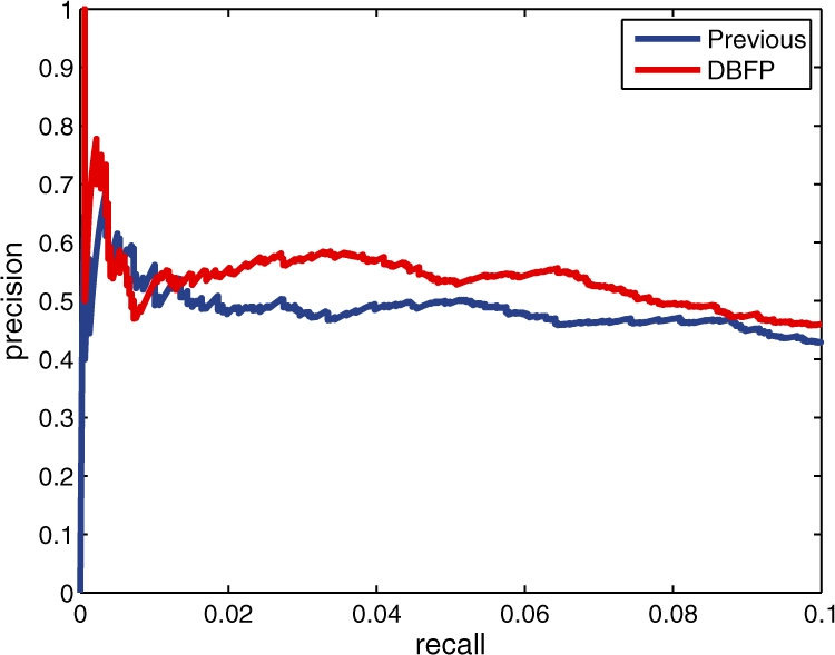
Precision-recall curves for footprint detection. The figure plots the precision-recall curves (up to a recall of 0.1) for DBFP and our previously described method.
3.2 Assignment of statistical confidence estimates
We proceeded to identify statistically significant footprints. As described in Section 2.3, we built an empirical null model to estimate a q-value for each footprint candidate located within the yeast intergenic regions. Table 1 shows the number of significant footprints identified at different q-value thresholds. At each q-value threshold t, the number of TPs can be estimated by multiplying (1 − t) by the number of predicted footprints. The resulting estimate is also shown in the table. At a q-value threshold of 0.05, 4679 footprints are considered significant, and the number of TPs is estimated to be 4445.
Table 1.
Significant footprints identified within the yeast intergenic regions
| q-value threshold | No. of footprints | No. of true positives | Previous prediction (%) | Unmappable ratio |
|---|---|---|---|---|
| 0.01 | 970 | 960 | 97.6 | 33.0 |
| 0.05 | 4679 | 4445 | 52.6 | 2.0 |
| 0.10 | 7784 | 7006 | 41.1 | 2.3 |
Each row lists a q-value threshold, the number of predicted footprints, the estimated number of true positives, the percentage of footprint bases covered by the previous prediction, and the ratio of the percentage of unmappable bases between the DBFP prediction and the previous prediction.
Table 1 also lists the results of comparing the prediction of DBFP with our previous prediction (Hesselberth et al., 2009). We first computed, at each q-value threshold, the percentage of bases in all DBFP footprints that are covered by the previous prediction. Almost all of the most significant footprints (i.e. those of q-value <0.01) are covered by both predictions, and when turning to a less stringent q-value cutoff, nearly half of the bases in the DBFP prediction are covered by the previous prediction. We next computed, at each q-value threshold, the percentage of unmappable bases in the DBFP prediction and the previous prediction, respectively, and took the ratio of these two percentages. DBFP consistently includes more unmappable bases in its prediction than the previous algorithm does. This is because, in contrast to the ad hoc greedy procedure, the DBN model explicitly treats unmappable positions as missing data and handles them in a probabilistic manner.
3.3 Footprints are enriched upstream of TSSs
We analyzed the genomic locations of identified footprints with respect to TSSs (Lee et al., 2007). Figure 5 plots the distribution of the distance from each footprints to the closest TSS. Reassuringly, the identified footprints are enriched in the region from 300 bp upstream to 100 bp downstream of TSSs. Furthermore, as the q-value threshold becomes more stringent, the identified footprints show a higher enrichment around 100 bp upstream of TSSs.
Fig. 5.
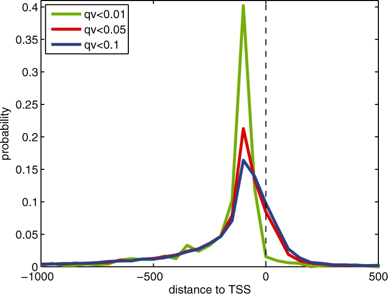
The distribution of distances from footprints to their closest TSSs. The footprints are identified according to three different q-value thresholds, 0.01, 0.05 and 0.1.
3.4 Footprints are enriched for known motifs
We next searched the 4679 fooprints identified at q-value <0.05 for sequences that match the TF binding motifs derived from in vivo ChIP-Chip experiments by MacIsaac et al. (2006) and those derived from in vitro protein-binding microarray (PBM) experiments by Zhu et al. (2009). The motif scanning tool FIMO was used for this analysis. At a scanning q-value threshold of 0.05, 35.7% of the 4679 footprints overlap a MacIsaac/Zhu motif. For each MacIsaac/Zhu motif that have at least five occurrences in our identified footprints, Table 2 lists its number of occurrences and the number of footprints containing the motif. When we expanded our search to include yeast motifs from TRANSFAC version 12.1, the percentage of motif-containing footprints increases to 36.8%. Figure 6 plots this percentage as a function of the FIMO q-value threshold and the footprint q-value threshold, respectively.
Table 2.
Numbers of occurrences of MacIsaac and Zhu motifs in the identified footprints
| TF | Source | No. of occurrences | No. of footprints | Enrichment |
|---|---|---|---|---|
| Sfp1 | Z | 915 | 339 | 6.16 |
| M | 172 | 160 | 12.57 | |
| Reb1 | M | 551 | 542 | 14.14 |
| Abf1 | M | 458 | 447 | 11.50 |
| Stb2 | M | 419 | 414 | 16.62 |
| Rap1 | M | 211 | 189 | 5.55 |
| Z | 76 | 75 | 4.66 | |
| Fhl1 | M | 106 | 104 | 11.61 |
| Rsc30 | Z | 100 | 44 | 2.17 |
| Mcm1 | M | 49 | 33 | 3.11 |
| Z | 38 | 22 | 3.71 | |
| Yrr1 | M | 46 | 46 | 7.84 |
| Stb3 | Z | 43 | 43 | 2.48 |
| Azf1 | M | 32 | 32 | 1.11 |
| Tye7 | Z | 29 | 17 | 2.75 |
| Hsf1 | M | 19 | 15 | 4.47 |
| Rsc3 | Z | 15 | 8 | 1.86 |
| Hal9 | Z | 13 | 7 | 2.66 |
| Snf1 | M | 12 | 11 | 1.73 |
| Stp2 | Z | 12 | 10 | 1.83 |
| Ume6 | M | 12 | 12 | 1.63 |
| Z | 9 | 9 | 1.25 | |
| Snt2 | M | 10 | 10 | 1.33 |
| Ydr520c | M | 9 | 6 | 2.51 |
| Uga3 | M | 8 | 4 | 3.08 |
| Tbs1 | Z | 7 | 5 | 1.17 |
| Mbp1 | Z | 6 | 6 | 2.19 |
| Cha4 | Z | 6 | 6 | 1.90 |
| Asg1 | Z | 6 | 5 | 1.85 |
| Dal81 | M | 5 | 4 | 3.37 |
| Cbf1 | Z | 5 | 4 | 2.28 |
Each row lists the name of a known TF binding motif, the source of that motif (M stands for MacIsaac motifs and Z stands for Zhu motifs), the number of its occurrences in the footprints, the number of footprints in which that motif appears, as well as the enrichment of the motif in the footprints with respect to the yeast intergenic regions. The motif occurrences are identified with a scanning q-value threshold 0.05.
Fig. 6.
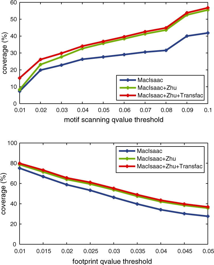
Percentage of footprints containing known motifs. Given the set of footprints with q-value <0.05, the top plot illustrates how the percentage of footprints that contain known motifs varies with the scanning q-value threshold used by FIMO. At a fixed motif scanning q-value threshold 0.05, the bottom plot illustrates how the percentage of identified footprints that contain known motifs varies with the footprint q-value threshold. Three categories of known motifs are used: (i) the MacIsaac motifs; (ii) both the MacIsaac motifs and the Zhu motifs; (iii) the MacIsaac motifs, the Zhu motifs and the yeast motifs in the TRANSFAC database.
Table 2 also lists the enrichment of each motif in the footprints relative to the yeast intergenic regions. For this analysis, the footprints and the yeast intergenic regions were scanned, respectively against the MacIsaac/Zhu motifs at a p-value threshold of 10−5. The enrichment of a motif is then defined as the ratio between the average number (per base pair) of occurrences of the motif in the footprints and that in the intergenic regions. Notably, all motifs in the table show an enrichment > 1.0. Furthermore, some motifs, including Sfp1, Reb1, Abf1, Stb2 and Fhl1, have more than 10-fold enrichments. These enrichment results indicate that the footprints are densely populated with protein-binding motifs. Finally, it is noteworthy that the Zhu motifs tend to have a lower enrichment than the MacIsaac motifs.
3.5 Footprints with no known motifs co-occur with footprints containing known motifs
Of our 4679 footprints, 1724 can be linked to a known TF binding motif in the MacIsaac data set, the Zhu data set or TRANSFAC. We expect roughly 234 of the 4679 footprints to be false positives, based upon the q-value threshold of 0.05. Some of the remaining 2721 footprints may correspond to non-sequence-specific binding mediated by a nearby sequence-specific binding event.
To test this hypothesis, we computed, for each footprint, the distance from that footprint to its nearest footprint neighbor. A footprint is called isolated if its distance to the nearest neighbor is larger than a given threshold. We then partitioned our collection of 4679 footprints into two subsets: (i) 1724 ones that contain a known protein-binding motif at q-value <0.05, called known footprints; and (ii) 2955 ones that do not, called unknown footprints. Finally, we counted how many footprints in each of these two subsets are isolated with respect to a given isolation threshold. The results of this analysis are shown in Figure 7 with the isolation threshold varying from 0 to 200 bp . The figure illustrates that, when the isolation threshold is >20 bp, a higher fraction of known footprints are isolated than that of unknown footprints. This observation supports the hypothesis that, at least for a fraction of the footprints that contain no known protein-binding motif, the footprint is maintained in part by the presence of proximal binding events with higher sequence specificity.
Fig. 7.
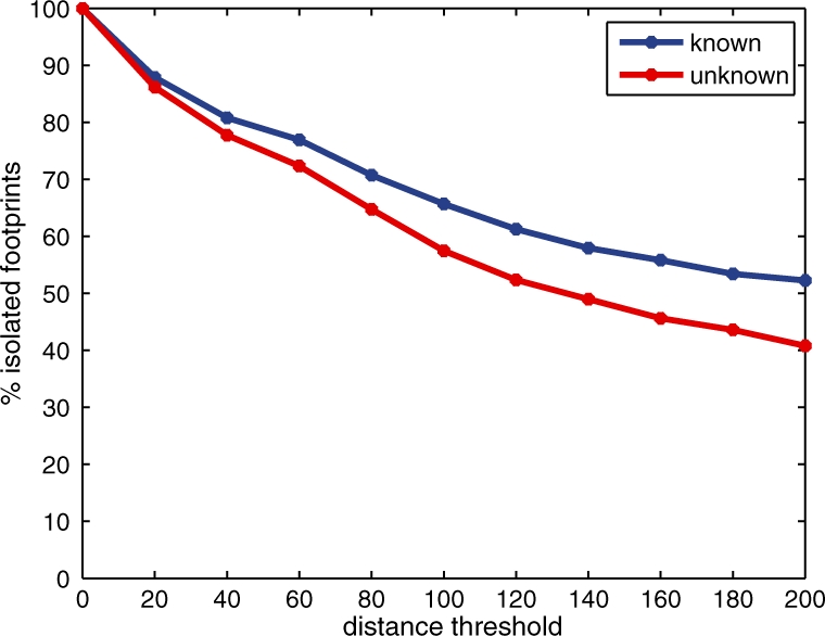
Footprints that do not contain a known motif tend to occur close to a second footprint. The figure plots the percentage of footprints that are isolated as a function of the isolation threshold in base pairs. The two series correspond to footprints that contain a known motif and footprints that do not.
We next focus on a subset of known footprints that are proximal to an unknown footprint with respect to a given distance threshold, called proximal known footprints. This subset of known footprints presumably contains motifs that are required to mediate the non-specific binding revealed by the unknown footprints. Therefore, we seek to identify known motifs that are enriched in those proximal known footprints. For this analysis, we considered MacIsaac, Zhu and TRANSFAC motifs, and various distance thresholds including 50, 100, 150 and 200 bp. Given a known motif and a distance threshold, we counted the occurrences of that motif in the proximal known footprints and in all known motifs, respectively, and then calculated a hypergeometric p-value to measure the enrichment of that motif in the proximal known footprints with respect to all known footprints.
At a distance threshold 200 bp, Mcm1 (MacIsaac motif) was identified as an enriched motif with a p-value = 0.01. This suggests that Mcm1 tends to collaborate with some non-specific binding proteins, which is consistent with the fact that Mcm1 is a cofactor of multiple TFs (Dolan et al., 1989; Jarvis et al., 1989; Keleher et al., 1989; Mead et al. 2002). One candidate factor for these footprints is Ste12, which is produced in haploid cells and binds cooperatively with Mcm1 to regulate mating and cell fusion-specific genes (Mead et al., 2002).
At distance thresholds 50 bp and 100 bp, Sfp1 (Zhu motif) was identified as an enriched motif with p-values 5.92 × 10⁻⁵ and 2.12 × 10⁻³, respectively. Sfp1 is a TF that integrates nutrient information and stress signals to control the expression of ribosomal protein genes. Previous Sfp1 ChIP experiments indicated that Sfp1 binds the promoters of some, but not all genes whose expression is dependent on Sfp1, suggesting that it may not directly bind DNA (Marion et al., 2004). However, Sfp1 exhibits sequence-specific binding in PBM experiments (Zhu et al., 2009). The occurrence of Sfp1-associated footprints with proximal unknown footprints suggests that Sfp1 might bind DNA weakly in cooperation with another unknown factor to regulate gene expression.
3.6 Footprints detected in coding regions
Thus far, our analysis has focused on footprints detected within intergenic regions of the yeast genome. However, we expect some protein binding events to occur in coding regions. Therefore, we estimated q-values for all footprint candidates across the whole yeast genome. Within the yeast coding regions, DBFP identified 50 footprints with q<0.01 and 1238 footprints with q<0.05.
Perocchi et al. (2007) recently described a collection of 206 antisense RNA transcripts that occur within coding regions of the S. cerevisiae genome. To detect binding events associated with such transcripts, we searched for footprints located from 300 bp upstream to 100 bp downstream of the TSSs of the 206 transcripts. In this way, we identified 22 footprints that occur near the TSSs of 15 antisense transcripts. Those footprints are potential regulatory regions for the nearby antisense transcripts. Table 3 reports the top ten antisense transcripts that are associated with significant footprints. For each antisense transcript, the table lists the gene in which that transcript occurs, the associated footprints, the footprint q-value, and the distance from the associated footprint to the TSS of that transcript. Notably, all footprints in Table 3 occur upstream of their corresponding antisense transcripts. A Reb1 footprint upstream of the GAL10 antisense RNA is required for its transcription (Houseley et al., 2008), suggesting that these other antisense RNA-associated footprints may function similarly.
Table 3.
Footprints associated with antisense transcripts
| Antisense transcripts | Gene | Footprint | q-value | Distance |
|---|---|---|---|---|
| chr7:272411-272907(−) | MET13 | chr7:272981-272998 | 0.003 | −74 |
| chr7:273063-273082 | 0.014 | −156 | ||
| chr11:66488-67632(+) | MNN4 | chr11:66368-66389 | 0.004 | −99 |
| chr1:43429-45165(+) | ACS1 | chr1:43241-43270 | 0.019 | −159 |
| chr13:140421-141541(+) | ERV41 | chr13:140165-140175 | 0.028 | −246 |
| chr8:3567034-358136(−) | NDT80 | chr8:358317−358346 | 0.030 | −181 |
| chr8:358214-358221 | 0.034 | −78 | ||
| chr7:753287-753351(+) | YGR130C | chr7:753005-753027 | 0.034 | −260 |
| chr6:89565-90613(+) | EPL1 | chr6:89297-89326 | 0.035 | −239 |
| chr1:189415-191399(−) | YAT1 | chr1:191594-191602 | 0.036 | −195 |
| chr12:323473-325185(−) | SUL2 | chr12:325274-325283 | 0.038 | −89 |
| chr2:276748-278764(+) | GAL10 | chr2:276585-276608 | 0.039 | −140 |
Each row lists an antisense transcript (+ and − in parentheses indicate the transcript orientation), the gene in which that transcript occur, the associated footprint, the footprint q-value, and the distance from the associated footprint to the TSS of that transcript.
Because the DNAseI experiment was primarily designed for detecting footprints in regions of high chromatin accessibility, the sequencing coverage in coding regions is much lower than that in intergenic regions (details in Section 2.5). Because of this low converage, we focus on the most significant footprints to search for known motifs. Among the 50 footprints with q-value <0.01, we observe that 60% contain a MacIsaac/Zhu/TRANSFAC motif at a scanning q-value threshold 0.05. Furthermore, Abf1 and Rap1 motifs are highly enriched in this set of footprints: 36% of the 50 footprints overlap an Abf1 site, while 12% of them overlap a Rap1 site. Both Abf1 and Rap1 are chromatin-associated factors with known roles in establishing open chromatin (Devlin et al., 1991; Lascaris et al., 2000; Yarragudi et al., 2004). The enrichment of Abf1 and Rap1 motifs suggests that these factors may be recruited to create nucleosome-free regions in open reading frames to facilitate the binding of other proteins. This observation in turn suggests that the footprints detected in coding regions with high confidence are likely regulatory regions.
4 DISCUSSION
We have developed a DBN-based approach for detecting protein-binding footprints from digital genomic footprinting data. Based on a previously described depletion scoring function and an empirical null model, we assign a statistical confidence score to each predicted footprint. Although our approach is primarily designed for the digital footprinting data of yeast, it will scale well to large genomes. For example, our DBN model handles unmappable positions in a probabilistic framework rather than simply ignoring them. This is important because unmappable positions in digital footprinting data can significantly affect footprint detection, particularly for eukaryotic organisms that tend to have an increased proportion of unmappable positions. As the technique of genomic digital footprinting is being applied to an increased number of organisms, DBFP can be readily applied to identify protein-binding footprints and regulatory elements for any organism.
We applied DBFP to the DNaseI cleavage data of the yeast genome and detected 4679 footprints within the intergenic regions at a q-value threshold of 0.05. The identified footprints are preferentially located in promoter regions. Furthermore, the footprints are enriched for TFBSs, with 36.8% of them overlapping at least one known motif. Our results show that footprints that do not contain known binding sites tend to be located close to a second footprint. As such, the unknown footprints may correspond to non-specific binding events that are facilitated by an adjacent specific binding event.
Within coding regions, DBFP identified many significant footprints near the TSSs of previously described antisense transcripts. Focusing further on the most significant footprints, our analysis reveals strong enrichment of Abf1 and Rap1 binding sites. We conjecture that these two TFs may be recruited to open chromatin in coding regions and increase the binding affinity of other proteins.
As shown in Figure 6, even at a loose scanning q-value threshold of 0.1 and even considering the combined database of MacIsacc, Zhu, and TRANSFAC motifs, less than 60% of the 4679 footprints that we identified with q-value < 0.05 can be associated with a known TF binding motif. This somewhat surprisingly low coverage can be explained in various ways. First, some sequence motifs may be poorly characterized or may lack sufficient intrinsic specificity to allow them to be identified with confidence. Second, some footprints may correspond to non-specific binding, as described in Section 3.5. Third, some footprints may be FP calls made by our algorithm. Indeed, approximately 234 of the 4,679 footprints are estimated to be FPs. Last, some of the footprints may correspond to previously uncharacterized protein-binding motifs. To address this possibility, we searched our identified footprints for novel motifs. We discovered two more variants of the Reb1 motif and several candidate novel binding motifs that need to be further validated (see Supplementary Material for details).
In our analysis, we considered only those bases that are mappable on both DNA strands. If the two strands are treated separately in the score calculations, then we could retain the tags assigned to positions that are mappable on only a single strand. However, we discarded those single-strand tags for two reasons. First, we observed that the distribution of the number of tags on one strand is strongly dependent upon the number of tags on the opposite strand (data not shown). Treating the two strands separately would ignore this dependency. Second, single-strand mappable positions tend to occur in clusters, corresponding to the edges of unmappable regions. It would be difficult to replicate such clusters in our empirical null model. Given the fact that only 3% of all mappable positions are mappable on a single strand, we opted to simply discard those positions.
We have described in Section 2.2 a score function that computes the probability of observing x or fewer tags based on the binomial distribution, assuming the tags are randomly drawn according to a uniform background distribution. With the same assumption, we can also calculate the depletion score as the probability of observing x or fewer tags based on the Poisson distribution. Because the binomial distribution converges to the Poisson distribution as the number of trials approaches infinity, these two scoring schemes are closely related. However, when we switched from a binomial to Poisson score function, we observed that the Poisson-based scores performed slightly worse than the binomial-based scores (data not shown).
To identify significant footprints, we built an empirical null model for q-value estimation by shuffling genomic positions. An alternative way to build the null model is to shuffle individual tags. However, shuffling individual tags leads to changes in the distribution of positional tag counts. We observed from the real data that the variance of positional tag counts is quite large. After shuffling individual tags, this variance decreases considerably. Therefore, a null model based on this type of shuffling would result in liberal q-values. Moreover, after shuffling individual tags, the rank transformation described in Section 2.2 has a different effect on the real data and on the null data. For the real data, the rank transformation reduces the large difference of tag counts among genomic positions; for the null data, in which positional tag counts have small variance, the rank transformation actually exaggerates the small difference of tag counts among the positions. Due to the reasons described above, we chose to shuffle genomic positions instead of individual tags.
Supplementary Material
ACKNOWLEDGEMENTS
The authors thank Sheila Reynolds for helpful discussion.
Funding: National Science Foundation award DBI 085008; National Institute of Health/National Center for Research Resources award P41 RR0011823; National Science and Engineering Research Council of Canada scholarship PGS D3.
Conflict of Interest: none declared.
REFERENCES
- Bilmes J, Bartels C. Graphical model architectures for speech recognition. IEEE Signal Processing Magazine. 2005;22:89–100. [Google Scholar]
- Bilmes J, Zweig G. Proceedings of the IEEE International Conference on Acoustics, Speech, and Signal Processing. Orlando, USA: 2002. The Graphical Models Toolkit: An open source software system for speech and time-series processing; pp. 3916–3919. [Google Scholar]
- Devlin C, et al. RAP1 is required for BAS1/BAS2- and GCN4-dependent transcription of the yeast HIS4 gene. Mol. Cell Biol. 1991;11:3642–3651. doi: 10.1128/mcb.11.7.3642. [DOI] [PMC free article] [PubMed] [Google Scholar]
- Dolan JW, et al. The yeast STE12 protein binds to the DNA sequence mediating pheromone induction. Proc. Natl Acad. Sci. USA. 1989;86:5703–5707. doi: 10.1073/pnas.86.15.5703. [DOI] [PMC free article] [PubMed] [Google Scholar]
- Dorschner MO, et al. High-throughput localization of functional elements by quantitative chromatin profiling. Nat. Methods. 2004;1:219–225. doi: 10.1038/nmeth721. [DOI] [PubMed] [Google Scholar]
- Hesselberth JR, et al. Global mapping of protein-DNA interactions in vivo by digital genomic footprinting. Nat. Methods. 2009;6:283–289. doi: 10.1038/nmeth.1313. [DOI] [PMC free article] [PubMed] [Google Scholar]
- Houseley J, et al. A ncRNA modulates histone modification and mrna induction in the yeast GAL gene cluster. Mol. Cell. 2008;32:685–695. doi: 10.1016/j.molcel.2008.09.027. [DOI] [PMC free article] [PubMed] [Google Scholar]
- Jarvis EE, et al. The yeast transcription activator PRTF, a homolog of the mammalian serum response factor, is encoded by the MCM1 gene. Genes Dev. 1989;3:936–945. doi: 10.1101/gad.3.7.936. [DOI] [PubMed] [Google Scholar]
- Johnson DS, et al. Genome-wide mapping of in vivo protein-DNA interactions. Science. 2007;316:1497–1502. doi: 10.1126/science.1141319. [DOI] [PubMed] [Google Scholar]
- Keleher CA, et al. Yeast repressor alpha 2 binds to its operator cooperatively with yeast protein Mcm1. Mol. Cell Biol. 1989;9:5228–5230. doi: 10.1128/mcb.9.11.5228. [DOI] [PMC free article] [PubMed] [Google Scholar]
- Klammer AA, et al. Modelling peptide fragmentation with dynamic Bayesian networks yields improved tandem mass spectrum identification. Bioinformatics. 2008;24:i345–i356. doi: 10.1093/bioinformatics/btn189. [DOI] [PMC free article] [PubMed] [Google Scholar]
- Lascaris RF, et al. Different roles for abf1p and a T-rich promoter element in nucleosome organization of the yeast RPS28A gene. Nucleic Acids Res. 2000;28:1390–1396. doi: 10.1093/nar/28.6.1390. [DOI] [PMC free article] [PubMed] [Google Scholar]
- Lee W, et al. A high-resolution atlas of nucleosome occupancy in yeast. Nat. Genet. 2007;39:1235–1244. doi: 10.1038/ng2117. [DOI] [PubMed] [Google Scholar]
- MacIsaac KD, et al. An improved map of conserved regulatory sites for saccharomyces cerevisiae. BMC Bioinformatics. 2006;7:113. doi: 10.1186/1471-2105-7-113. [DOI] [PMC free article] [PubMed] [Google Scholar]
- Marion RM, et al. Sfp1 is a stress- and nutrient-sensitive regulator of ribosomal protein gene expression. Proc. Natl Acad. Sci. USA. 2004;101:14315–14322. doi: 10.1073/pnas.0405353101. [DOI] [PMC free article] [PubMed] [Google Scholar]
- Mavrich TN, et al. A barrier nucleosome model for statistical positioning of nucleosomes throughout the yeast genome. Genome Res. 2008;18:1073–1083. doi: 10.1101/gr.078261.108. [DOI] [PMC free article] [PubMed] [Google Scholar]
- Mead J, et al. Interactions of the Mcm1 MADS box protein with cofactors that regulate mating in yeast. Mol. Cell Biol. 2002;22:4607–4621. doi: 10.1128/MCB.22.13.4607-4621.2002. [DOI] [PMC free article] [PubMed] [Google Scholar]
- Perocchi F, et al. Antisense artifacts in transcriptome microarray experiments are resolved by actinomycin D. Nucleic Acids Res. 2007;35:e128. doi: 10.1093/nar/gkm683. [DOI] [PMC free article] [PubMed] [Google Scholar]
- Ren B, et al. Genome-wide location and function of DNA binding proteins. Science. 2000;290:2306–2309. doi: 10.1126/science.290.5500.2306. [DOI] [PubMed] [Google Scholar]
- Reynolds SM, et al. Transmembrane topology and signal peptide prediction using dynamic bayesian networks. PLoS Comput. Biol. 2008;4:e1000213. doi: 10.1371/journal.pcbi.1000213. [DOI] [PMC free article] [PubMed] [Google Scholar]
- Robertson G, et al. Genome-wide profiles of STAT1 DNA association using chromatin immunoprecipitation and massively parallel sequencing. Nat. Methods. 2007;4:651–657. doi: 10.1038/nmeth1068. [DOI] [PubMed] [Google Scholar]
- Staden R. Searching for motifs in nucleic acid sequences. Methods Mol. Biol. 1994;25:93–102. doi: 10.1385/0-89603-276-0:93. [DOI] [PubMed] [Google Scholar]
- Storey JD, Tibshirani R. Statistical significance for genome-wide studies. Proc. Natl Acad. Sci. USA. 2003;100:9440–9445. doi: 10.1073/pnas.1530509100. [DOI] [PMC free article] [PubMed] [Google Scholar]
- Valouev A, et al. Genome-wide analysis of transcription factor binding sites based on Chip-Seq data. Nat Methods. 2008;5:829–834. doi: 10.1038/nmeth.1246. [DOI] [PMC free article] [PubMed] [Google Scholar]
- Wu C. The 5' ends of Drosophila heat shock genes in chromatin are hypersensitive to DNase I. Nature. 1980;286:854–860. doi: 10.1038/286854a0. [DOI] [PubMed] [Google Scholar]
- Yao X.-Q, et al. A dynamic Bayesian network approach to protein secondary structure prediction. BMC Bioinformatics. 2008;9:49. doi: 10.1186/1471-2105-9-49. [DOI] [PMC free article] [PubMed] [Google Scholar]
- Yarragudi A, et al. Comparison of ABF1 and RAP1 in chromatin opening and transactivator potentiation in the budding yeast saccharomyces cerevisiae. Mol. Cell Biol. 2004;24:9152–9164. doi: 10.1128/MCB.24.20.9152-9164.2004. [DOI] [PMC free article] [PubMed] [Google Scholar]
- Zhu C, et al. High-resolution DNA-binding specificity analysis of yeast transcription factors. Genome Res. 2009;19:556–566. doi: 10.1101/gr.090233.108. [DOI] [PMC free article] [PubMed] [Google Scholar]
Associated Data
This section collects any data citations, data availability statements, or supplementary materials included in this article.