Abstract
Motivation: Circadian rhythms are prevalent in most organisms. Identification of circadian-regulated genes is a crucial step in discovering underlying pathways and processes that are clock-controlled. Such genes are largely detected by searching periodic patterns in microarray data. However, temporal gene expression profiles usually have a short time-series with low sampling frequency and high levels of noise. This makes circadian rhythmic analysis of temporal microarray data very challenging.
Results: We propose an algorithm named ARSER, which combines time domain and frequency domain analysis for extracting and characterizing rhythmic expression profiles from temporal microarray data. ARSER employs autoregressive spectral estimation to predict an expression profile's periodicity from the frequency spectrum and then models the rhythmic patterns by using a harmonic regression model to fit the time-series. ARSER describes the rhythmic patterns by four parameters: period, phase, amplitude and mean level, and measures the multiple testing significance by false discovery rate q-value. When tested on well defined periodic and non-periodic short time-series data, ARSER was superior to two existing and widely-used methods, COSOPT and Fisher's G-test, during identification of sinusoidal and non-sinusoidal periodic patterns in short, noisy and non-stationary time-series. Finally, analysis of Arabidopsis microarray data using ARSER led to identification of a novel set of previously undetected non-sinusoidal periodic transcripts, which may lead to new insights into molecular mechanisms of circadian rhythms.
Availability: ARSER is implemented by Python and R. All source codes are available from http://bioinformatics.cau.edu.cn/ARSER
Contact: zhensu@cau.edu.cn
1 INTRODUCTION
Circadian rhythm is one of the most well-studied periodic processes in living organisms. DNA microarray technologies have often been applied in circadian rhythm studies (Duffield, 2003). Thus, we can monitor the mRNA expression of the whole-genome level, which is an effective way to simultaneously identify many hundreds or thousands of periodic transcripts. The matter to be addressed is which genes are rhythmically expressed based on their gene expression profiles. This can be classified as a periodicity identification problem. However, there are computational challenges when dealing with this issue: sparse determination of sampling rate, and short periods of data collection for microarray experiments (Bar-Joseph, 2004). Circadian microarray experiments are usually designed to collect data every 4 h over a course of 48 h, generating expression profiles with 12 or 13 time-points (Yamada and Ueda, 2007). There are two main factors that limit the number of data points that can be feasibly obtained: budget constraints and dampening of the circadian rhythm (Ceriani et al., 2002). Such short time-series data render many methods of classical time-series analysis inappropriate, since they generally require much larger samples to generate statistically significant results.
A variety of algorithms have been developed and applied to microarray time-series analysis; Chudova et al. (2009) indicated that the existing technologies fall into two major categories: time-domain and frequency-domain analyses. Typical time-domain methods rely on sinusoid-based pattern matching technology, while frequency-domain methods are based on spectral analysis methods. Of the time-domain methods, COSOPT (Straume, 2004) is a well-known algorithm frequently used to analyze circadian microarray data in Arabidopsis (Edwards et al., 2006), Drosophila (Ceriani et al., 2002) and mammalian systems (Panda et al., 2002). COSOPT measures the goodness-of-fit between experimental data and a series of cosine curves of varying phases and period lengths. The advantages of pattern-matching methods are simplicity and computational efficiency, while they are not effective at finding periodic signals that are not perfectly sinusoidal (Chudova et al., 2009).
Of the frequency-domain methods, Fisher's G-test was proposed to detect periodic gene expression profiles by Wichert et al. (2004) and has been used to analyze circadian microarray data of Arabidopsis (Blasing et al., 2005) and mammalian systems (Hughes et al., 2009; Ptitsyn et al., 2006). Fisher's G-test searches periodicity by computing the periodogram of experimental data and tests the significance of the dominant frequency using Fisher's G-statistic; however, it is limited by low frequency resolution for short time-series generated by circadian microarray experiments, which means it is often not adequate to resolve the periodicity of interest (Langmead et al., 2003). Time-domain and frequency-domain methods are two different ways to analyze the time-series, each with advantages and disadvantages. Frequency-domain methods are noise-tolerant and model-independent but their results are difficult for biologists to understand. Time-domain methods can give comprehensive and easily-understood descriptions for rhythms but are noise-sensitive and model-dependent (e.g. sinusoid).
Considering the above limitations, we propose an algorithm named ARSER that combines time-domain and frequency-domain analyses to identify periodic transcripts in large-scale time-course gene expression profiles. ARSER employs autoregressive (AR) spectral analysis (Takalo et al., 2005) to estimate the period length of a circadian rhythm from the frequency spectrum. It is well-suited to analyze short time-series since it can generate smooth and high-resolution spectra from gene expression profiles. It is related (but not identical) to a method called maximum entropy spectral analysis, which has been applied to the analysis of micorarray data (Langmead et al., 2002).
After the frequency-domain analysis, ARSER takes harmonic regression (Warner, 1998) to model the circadian rhythms extracted from gene expression profiles. Harmonic regression models fully describe the rhythms using four parameters: period (duration of one complete cycle), the mean level (the mid-value of the time-series), the amplitude (half the distance from the peak to the trough of the fitted cosine, indicating the predictable rise and fall around the mean level) and the phase (the location in time of the peak of the curve).
The joint strategy overcomes the shortcomings of separate time-domain or frequency-domain analyses. ARSER uses AR spectral analysis to find the circadian rhythms and a harmonic regression model to characterize and statistically validate them. When tested on multiple synthetic datasets, ARSER is robust to noise, quickly and exactly estimates periodicity and gives comprehensive and statistically significant results in analysis of short time-series.
This article is organized as follows. Section 2 describes the mathematical and implemental details of the ARSER algorithm. Section 3 compares the performance of ARSER with COSOPT and Fisher's G-test by testing on different simulation datasets. Numerical experiments are designed by varying noise intensity and period length, including random background models and identifying non-sinusoidal periodic patterns. Finally, ARSER was used to analyze Arabidopsis microarray data and obtained a novel set of rhythmic transcripts, many of which showed non-sinusoidal periodic patterns. Section 4 summarizes the methodology.
2 METHODS
2.1 Overview
Our methodology to detect circadian rhythms in gene expression profiles consists of three procedures: data pre-processing, period detection and harmonic regression modeling (Fig. 1A). First, ARSER performs a data preprocessing strategy called detrending that removes any linear trend from the time-series so that we can obtain a stationary process to search for cycles. Detrending is carried out by ordinary least squares (OLS). Second, ARSER determines the periods of the time-series within the range of circadian period length (20–28 h) (Piccione and Caola, 2002). The method to estimate periods is carried out by AR spectral analysis, which calculates the power spectral density of the time-series in the frequency domain. If there are cycles of circadian period length in the time-series, the AR spectral density curve will show peaks at each associated frequency (Fig. 1B). With the periods obtained from AR spectral analysis, ARSER employs harmonic regression to model the cyclic components in the time-series. Harmonic analysis provides the estimates of three parameters (amplitude, phase and mean) that describe the rhythmic patterns. Finally, when analyzing microarray data, false discovery rate q-values are calculated for multiple comparisons.
Fig. 1.
The diagram of our methodology (named ARSER) and a case study. (A) Analysis flowchart. First, data pre-processing by linear trend removal (detrending), then period detection by searching peaks from the AR spectrum. With the periods derived from the AR spectrum, harmonic regression is carried out to model circadian rhythms by fitting the detrended time-series with trigonometric functions. Finally, ARSER describes the periodicity by several parameters: period, phase, amplitude, statistical significance and so on. (B) An example of rhythmicity analysis by ARSER. The synthetic time-series is generated by the following equation:  , where t∈[0, 96] with 4 h intervals and ε is white noise following (μ=0, σ=40) normal distribution.
2.2 Period detection
As circadian rhythm has approximately (but never exactly) 24 h periodicity (Harmer, 2009), the first matter to be addressed is to measure the length of actual period for each gene expression profile.
ARSER estimates the period by AR spectral estimation, which is a high-resolution spectral analysis technique comparing with the classical fast Fourier transform periodogram. Given an equally sampled time-series {xt} with the sampling interval Δ, AR spectral estimation first applies an AR model of order p, abbreviated AR(p), to fit the time-series using the following equation:
| (1) |
where εt is white noise and αi are model parameters (or AR coefficients) with αp≠0 for an order p process. Güler et al. (2001) and Spyers-Ashby et al. (1998) reported that AR coefficients are generally estimated by three methods: the Yule–Walker method, maximum likelihood estimation and the Burg algorithm. ARSER implements the AR model-fitting by setting order p=24/Δ and computing the AR coefficients using all three methods.
After AR modeling, AR spectral analysis estimates the spectrum, with model parameters instead of original data, using the following equation:
| (2) |
where σε2 is the variance of white noise; αk are parameters defined in Equation (1). If periodic signals are present in the time-series, then the spectrum derived from Equation (2) will show peaks at dominant frequencies. However, at high frequencies the noise signals may also show peaks known as pseudo-periods.
ARSER obtains the period by using the following step-by-step procedure:
Remove the linear trend in time-series {xt}, denoting the detrended time-series as
 .
.Smooth
 by a fourth-order Savitzky–Golay algorithm (Savitzky and Golay, 1964). This is a low-pass filter that can efficiently remove pseudo-peaks in a spectrum caused by noise. The smoothed time-series is denoted as
  .
.Calculate the AR spectrum of
 by Equation (2), and select all periods
  that show peaks in the spectrum.
Calculate the AR spectrum of detrended time-series
 by Equation (2), and select all periods
  that show peaks in the spectrum.
The periods
 and
and  are chosen as input to the harmonic regression analysis for
  by Equation (3).
The optimum periods in {xt} are determined by Akaike's information criterion (Akaike, 1974) among the regression models generated in step 5.
2.3 Rhythm modeling and gene selection
The next matter to be addressed is how to model the rhythmic patterns in the time-series of gene expression. ARSER employs the harmonic regression model to represent the cycle trends, which involves fitting sinusoidal models to a time-series using the following equation:
| (3) |
where xt is the observed value at time t; μ is the mean level of the time-series; βi is the amplitude of the waveform; ϕi is the phase, or location of peaks relative to time zero; εt are residuals that are unrelated to the fitted cycles; and t are the sampling time-points.
The fi term in Equation (3) are the dominant frequencies in the circadian range derived by Equation (2). The periods (τi) of the time-series equal (1/fi)·Δ, where Δ is the sampling interval. Since periods are predetermined by AR spectral analysis, Equation (3) can be reduced to an even simpler multiple linear regression model:
| (4) |
where pi = βi cos ϕi, qi = −βi sin ϕi. The unknown parameters pi, qi and μ can be estimated by OLS method. Then the amplitude βi and phase ϕi are obtained by  and tan ϕi = −qi/pi.
By applying a harmonic regression model, rhythmicity in a time-series is fully described by four parameters: period, phase, amplitude and mean level. Tests of statistical significance are also essential to distinguish between real rhythms and random oscillations. In a harmonic regression model, an F-test is employed to assess the significance of pi and qi coefficients, and so statistically validates the rhythmicity.
When analyzing microarray expression data, tens of thousands of genes will be estimated simultaneously, so the problem of multiple testing must be considered. We employed the method of Storey and Tibshirani (2003). Briefly, by examining the distribution of P-values from the given dataset, an estimate of the proportion that are truly non-rhythmic can be derived. The P-value for each transcript can be converted to a more stringent q-value which represents the false discovery rate. In our study, we consider genes with q < 0.05 to be rhythmically expressed.
2.4 Generating simulation data
We provide a comprehensive testing strategy to test and compare the performance of ARSER with COSOPT and Fisher's G-test. Our simulation datasets consist of periodic and non-periodic time-series data. The periodic time-series was generated by two models based on the methods proposed by Robeva et al. (2008). One is classified as a stationary model, defined by
| (5) |
where SNR is signal-to-noise ratio; τ is period; ϕ is phase; and εt is (μ=0, σ=1) normally distributed noise terms. Another model classified as a non-stationary is defined by
| (6) |
where εt is (μ=0, σ=50) normally distributed noise; the mean level and amplitude exponentially decay over time. The periodic datasets used in our numerical experiments were generated by assigning different values to τ, ϕ and SNR. Compared with the stationary model, the non-stationary model is more likely to approximate the circadian rhythm (Refinetti, 2004).
The non-periodic time-series was generated from (μ=0, σ=1) normally distributed white noise and AR processes of order one, AR(1), as suggested by Futschik and Herzel (2008).
3 RESULTS AND DISCUSSION
ARSER was applied to both simulated and real microarray data. A series of numerical experiments were designed to test and compare the performance of ARSER with COSOPT and Fisher's G-test. The tasks were to (i) precisely estimate periodicity, (ii) separate periodic from non-periodic signals and (iii) identify non-sinusoidal periodic patterns.
3.1 Robustness to noise
In the first experiment, we compared the robustness of three algorithms to noise. We generated 10 000 stationary [derived from Equation (5)] and 10 000 non-stationary periodic signals [derived from Equation (6)] by the following steps: (i) taking τ by 0.1-h sampling interval in [20 h, 28 h), (ii) at each period, taking ϕ by 2π/25 sampling interval in [0, 2π) and (iii) at each period and phase, taking SNR of 5:1, 4:1, 3:1, 2:1 and 1:1. Each time-series possessed 12 data points, within 0–44 h at 4 h sampling intervals, which was the same as the majority of published circadian microarray datasets.
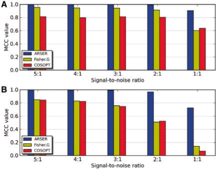
There were 2000 periodic time-series under each SNR. We also generated 2000 (μ=0, σ=1) normally distributed random signals. Then we applied ARSER, COSOPT and Fisher's G-test to identify periodic signals from the positive (periodic) and negative (random) samples and measured their performance of periodicity prediction under different SNRs by Matthew's correlation coefficient (MCC) (Fig. 2A and B). The MCC is in essence a correlation coefficient between the observed and predicted binary classifications, with values between −1 and +1. MCC = +1 represents a perfect prediction, 0 an average random prediction and −1 an inverse prediction (Baldi et al., 2000).
Fig. 2.
Accuracy of ARSER, COSOPT and Fisher's G-test at identifying (A) stationary and (B) non-stationary periodic signals under decreasing signal-to-noise ratio. For each group of periodic signals, there are 1:1 negative sample data generated by (μ=0, σ=1) white noise. The performance is measured by MCC. As noise intensity increased, ARSER (blue) performed robustly with noise in both situations, while COSOPT (red) and Fisher's G-test (yellow) performed badly for stationary periodic signals with high-level noise and even worse for non-stationary ones. They all scored the signals as periodic using the threshold of 0.05 for FDR q-value for ARSER and Fisher's G-test, or by pMMC-β for COSOPT. pMMC-β measures the probability for multiple testing, similarly to the FDR q-value.
Of the three methods, ARSER performed best at any noise-level for both stationary and non-stationary time-series, suggesting it was a robust periodicity detection algorithm.
3.2 Correctness for predicting wavelength
The task of precisely estimating periodicity included two parts: identification of truly periodic signals and the measurement of actual wavelength. The former case was verified for the three algorithms in the robustness experiment, and we continued to investigate the latter one.
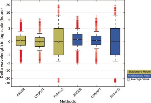
According to the predictions in the robustness experiment, we calculated the differences for each periodic signal in its actual period and predicted value by each algorithm. The distributions of prediction errors for the three algorithms (Fig. 3) showed that ARSER and COSOPT were more accurate (errors with zero means and small variations) in predicting the period length compared with Fisher's G-test (errors of large variation). This indicates ARSER and COSOPT are high-resolution detecting algorithms and can accurately estimate the wavelength of circadian rhythms.
Fig. 3.
Distribution of the differences between the predicted wavelength (using three algorithms) and the actual wavelength of stationary periodic signals (yellow) and non-stationary periodic signals (blue). Log transformation for the difference (Δτ) was carried out using ln(1+|Δτ|). The errors of wavelength prediction by ARSER and COSOPT were low and close to zero, while those for Fisher's G-test were high and in a wide range.
3.3 Periodicity detection with random background models
To verify our algorithm, our second task was to separate periodic from non-periodic signals, which measured the sensitivity and specificity in the predictions.
The periodic signals generated in the robustness experiment contained 10 000 stationary and 10 000 non-stationary time-series. The non-periodic signals were generated by white noise and AR(1) models with 10 000 samples in each case. Then we created four testing datasets by combining (i) stationary periodic signals with white noise signals, (ii) non-stationary periodic signals with white noise signals, (iii) stationary periodic signals with AR(1)-based random signals and (iv) non-stationary periodic signals with AR(1)-based random signals.
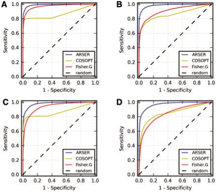
Since predictions were periodic or non-periodic, a well-suited binary classification, we applied receiver operating characteristic (ROC) curves (Fawcett, 2006) to compare the performances of the three algorithms on the four datasets (Fig. 4A–D). Performances were measured by the area under the ROC curve criterion, with the larger the area the better the method. ROC analysis showed that ARSER outperformed COSOPT and Fisher's G-test in all cases.
Fig. 4.
ROC curves for identifying periodic signals from four datasets of (A) 10 000 stationary periodic signals and 10 000 white noise signals, (B) 10 000 non-stationary periodic signals and 10 000 white noise signals, (C) 10 000 stationary periodic signals and 10 000 AR(1)-based random signals, and (D) 10 000 non-stationary periodic signals and 10 000 AR(1)-based random signals. Greater area under the ROC curve indicates better performance of the algorithm. ARSER gave the fewest false positives and false negatives compared with COSOPT and Fisher's G-test in all cases.
3.4 Detection of non-sinusoidal periodic waveforms
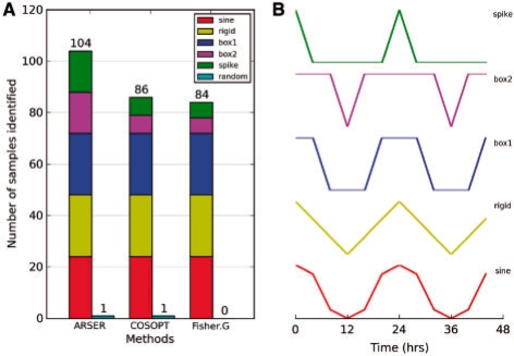
The last numerical experiment was to apply the three algorithms to detect non-sinusoidal periodic patterns. The testing dataset was downloaded from the HAYSTACK web site (http://haystack.cgrb.oregonstate.edu/). This dataset included five cycling patterns based on diurnal and circadian time-course studies: rigid, spike, sine and two box-like patterns (Michael et al., 2008). Each periodic pattern contained 24 samples with the phase shifted from 0 to 23 h by 1 h intervals. A total of 120 time-series were contained in the dataset, which possessed 12 time-points that represent two circadian cycles obtained at 4 h sampling intervals. We also added 120 (μ=0, σ=1) white-noise signals as negative data.
ARSER performed the best of the three algorithms (Fig. 5), and identified more spike and box-like periodic pattern profiles while maintaining a very low false positive rate.
Fig. 5.
Comparison of detecting multiple periodic waveforms. (A) Number of samples from five periodic waveforms and random signals (cyan) identified by three detecting algorithms. The testing dataset are composed of 120 periodic time-series with 24 samples for each periodic pattern and 120 (μ=0, σ=1) white-noise samples. (B) The waveforms include sinusoidal (red) and non-sinusoidal: rigid waves (yellow), box1 waves (blue), box2 waves (magenta) and spike waves (green). The dataset and periodic patterns were generated by HAYSTACK tool (Michael et al., 2008).
3.5 Analysis of Arabidopsis circadian expression data
Our methodology for identifying periodicity of short time-series worked successfully on synthetic datasets. We applied ARSER to analyze a real microarray dataset generated from the work of Edwards et al. (2006) in the study of the Arabidopsis circadian system. The data (available from http://millar.bio.ed.ac.uk/data.htm) are expression profiles of 13 data points, representing 48 h of observation obtained at 4 h sampling intervals. In the original study, the authors used COSOPT to identify cyclic genes. Of all 22 810 genes represented on the array, 3504 genes were considered rhythmic at the significance threshold pMMC-β <0.05.
We re-analyzed this microarray data using ARSER and Fisher's G-test, both of which scored rhythmic transcripts by FDR q<0.05, and compared their predictions with those of COSOPT (Fig. 6). ARSER identified 96% of the cycling transcripts identified by COSOPT, suggesting our methodology efficiently reproduced the original results, while Fisher's G-test merely identified only 15%, implying it may not efficiently analyze this circadian expression data.
Fig. 6.
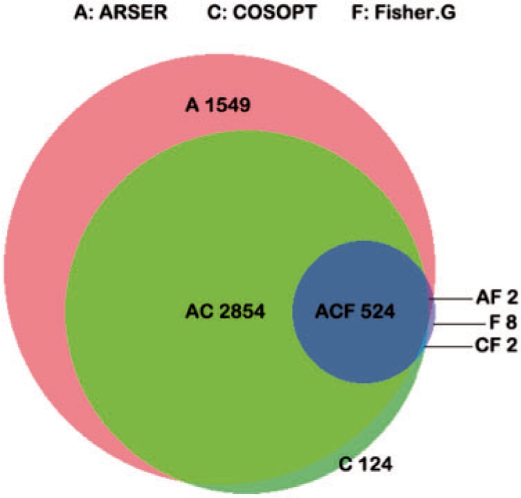
Area-proportional Venn diagram addresses the predictive power of three algorithms for identifying Arabidopsis circadian-regulated genes. The microarray data were originally analyzed by COSOPT in the study of Edwards et al. (2006), and scored 3504 genes as rhythmic (pMMC-β <0.05). A total of 4929 genes were identified by ARSER (FDR q<0.05), while only 536 were found by Fisher's G-test (FDR q<0.05). Venn diagram was generated by BioVenn tool (Hulsen et al., 2008).
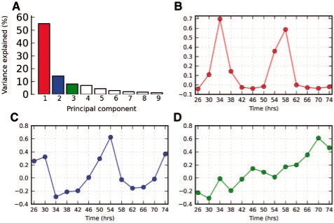
In addition, a novel set of 1549 transcripts were uniquely identified as rhythmic by ARSER. To examine these newly found genes more closely, we employed principal component analysis (Wall et al., 2003) to visualize the dominant expression patterns from their profiles. The first two principal components accounted for 70% of the variance (Fig. 7A) and were cyclic with spike-like patterns (Fig. 7B and C). These plots revealed a rhythmic component with a period of ∼24 h in many transcripts of the novel set, which was consistent with the estimate using ARSER. These periodic patterns were mainly non-sinusoidal and may explain why they were not identified by COSOPT in the original study. The third component also showed a linear trend (Fig. 7D), indicating the non-stationary feature of the data. Dodd et al. (2007) reported 27 well-known clock-associated genes in Arabidopsis. Two of these genes were found among the newly identified genes of the present study. One was CRYPTOCHROME 1 (CRY1), which functions as a photoreceptor for the circadian clock in a light-dependent fashion. In plants, the blue light photoreception can be used to cue developmental signals (Brautigam et al., 2004). The other one was PSEUDO-RESPONSE REGULATORS 9 (PRR9), which plays an important role in response to temperature signals in a temperature-sensitive circadian system (Harmer, 2009) and acted as transcriptional repressors of CCA1 and LHY in the feedback loop of the circadian clock (Nakamichi et al., 2010). Thus more clues could be provided by applying ARSER to further study of Arabidopsis circadian expression data.
Fig. 7.
Principal component analysis of the newly found rhythmic transcripts in Arabidopsis identified by ARSER. Plots of relative variance for the first nine components (A); and the first (B), second (C) and third (D) eigengenes are shown. The first three principal components account for 78% of the variance. The first and second eigengenes are cyclic with spike-like patterns, and the third shows a linear trend. These data reveal that non-sinusoidal and non-stationary periodic transcripts could be found by applying ARSER. PCA was carried out by Mev tool (Saeed et al., 2003).
Unlike the synthetic datasets used in numeral experiments, the notions of false positives and false negatives in real experimental data are not well defined. Thus, we used the 27 known clock genes as benchmark genes to evaluate a given algorithm in terms of false negatives for analyzing circadian expression data. We applied three algorithms to rank the 22 810 genes of the entire Arabidopsis genome in order of the statistical significance of their expression profiles. The rankings of the 27 known clock genes (Table 1) showed that the three algorithms performed similarly, and all identified most of the known clock genes from among their top 25% ranked candidates.
Table 1.
Summary of rankings of 27 known Arabidopsis clock-associated genes in the entire genome, in order of significance using three algorithms
| Method | Rankings in the entire genomea |
|||
|---|---|---|---|---|
| Top 5% | Top 10% | Top 25% | Top 60% | |
| ARSER | 10 | 15 | 21 | 26 |
| COSOPT | 11 | 16 | 20 | 24 |
| Fisher.G | 10 | 14 | 21 | 24 |
aARSER and Fiser's G-test rank genes by FDR q-value; COSOPT rank genes by pMMC-β.
4 CONCLUSION
In this study, we present an automated algorithm for identifying periodic patterns in large-scale temporal gene expression profiles. It employs harmonic regression based on AR spectral analysis to identify and model circadian rhythms. Compared with separate frequency-domain or time-domain methods, our methodology is a joint strategy which analyzes the time-series through both frequency and time domains. Testing on synthetic and real microarray data showed that our novel method was computationally optimal and substantially more accurate than two existing and widely-used rhythmicity detection techniques (COSOPT and Fisher's G-test). In addition, our method identifies a novel set of rhythmically expressed Arabidopsis genes which may supply more valuable information for further study of plant circadian systems.
ACKNOWLEDGEMENTS
We would like to thank Prof. John Hogenesch for sharing COSOPT software with us. We thank Gaihua Zhang for technical assistance. We thank Wenying Xu, Yi Ling, Daofeng Li, Jingna Si, Fei He and Tingyou Wang for helpful discussions.
Funding: Ministry of Science and Technology of China (2008AA02Z312, 2006CB100105).
Conflict of Interest: none declared.
REFERENCES
- Akaike H. A new look at the statistical model identification. IEEE Trans. Automat. Contr. 1974;19:716–723. [Google Scholar]
- Baldi P, et al. Assessing the accuracy of prediction algorithms for classification: an overview. Bioinformatics. 2000;16:412. doi: 10.1093/bioinformatics/16.5.412. [DOI] [PubMed] [Google Scholar]
- Bar-Joseph Z. Analyzing time series gene expression data. Bioinformatics. 2004;20:2493–2503. doi: 10.1093/bioinformatics/bth283. [DOI] [PubMed] [Google Scholar]
- Blasing O, et al. Sugars and circadian regulation make major contributions to global regulation of diurnal gene expression in Arabidopsis. Plant Cell. 2005;17:3257–3281. doi: 10.1105/tpc.105.035261. [DOI] [PMC free article] [PubMed] [Google Scholar]
- Brautigam C, et al. Structure of the photolyase-like domain of cryptochrome 1 from Arabidopsis thaliana. Proc. Natl Acad. Sci. 2004;101:12142. doi: 10.1073/pnas.0404851101. [DOI] [PMC free article] [PubMed] [Google Scholar]
- Ceriani M, et al. Genome-wide expression analysis in Drosophila reveals genes controlling circadian behavior. J. Neurosci. 2002;22:9305–9319. doi: 10.1523/JNEUROSCI.22-21-09305.2002. [DOI] [PMC free article] [PubMed] [Google Scholar]
- Chudova D, et al. Bayesian detection of non-sinusoidal periodic patterns in circadian expression data. Bioinformatics. 2009;25:3114–3120. doi: 10.1093/bioinformatics/btp547. [DOI] [PMC free article] [PubMed] [Google Scholar]
- Dodd AN, et al. The Arabidopsis circadian clock incorporates a cADPR-based feedback loop. Science. 2007;318:1789–1792. doi: 10.1126/science.1146757. [DOI] [PubMed] [Google Scholar]
- Duffield G. DNA microarray analyses of circadian timing: the genomic basis of biological time. J. Neuroendocrinol. 2003;15:991–1002. doi: 10.1046/j.1365-2826.2003.01082.x. [DOI] [PubMed] [Google Scholar]
- Edwards KD, et al. FLOWERING LOCUS C mediates natural variation in the high-temperature response of the Arabidopsis circadian clock. Plant Cell. 2006;18:639–650. doi: 10.1105/tpc.105.038315. [DOI] [PMC free article] [PubMed] [Google Scholar]
- Fawcett T. An introduction to ROC analysis. Pattern Recogn. Lett. 2006;27:861–874. [Google Scholar]
- Futschik ME, Herzel H. Are we overestimating the number of cell-cycling genes? The impact of background models on time-series analysis. Bioinformatics. 2008;24:1063–1069. doi: 10.1093/bioinformatics/btn072. [DOI] [PubMed] [Google Scholar]
- Güler İ., et al. AR spectral analysis of EEG signals by using maximum likelihood estimation. Comput. Biol. Med. 2001;31:441–450. doi: 10.1016/s0010-4825(01)00022-1. [DOI] [PubMed] [Google Scholar]
- Harmer SL. The circadian system in higher plants. Ann. Rev. Plant Biol. 2009;60:357–377. doi: 10.1146/annurev.arplant.043008.092054. [DOI] [PubMed] [Google Scholar]
- Hughes ME, et al. Harmonics of circadian gene transcription in mammals. PLoS Genet. 2009;5:e1000442. doi: 10.1371/journal.pgen.1000442. [DOI] [PMC free article] [PubMed] [Google Scholar]
- Hulsen T, et al. BioVenn – a web application for the comparison and visualization of biological lists using area-proportional Venn diagrams. BMC Genomics. 2008;9:488. doi: 10.1186/1471-2164-9-488. [DOI] [PMC free article] [PubMed] [Google Scholar]
- Langmead C, et al. Proceedings of IEEE Computer Society Bioinformatics Conference (CSB). Palo Alto, CA: Stanford University; 2002. A maximum entropy algorithm for rhythmic analysis of genome-wide expression patterns; pp. 237–245. (August 14–16) [PubMed] [Google Scholar]
- Langmead C, et al. Phase-independent rhythmic analysis of genome-wide expression patterns. J. Comput. Biol. 2003;10:521–536. doi: 10.1089/10665270360688165. [DOI] [PubMed] [Google Scholar]
- Michael TP, et al. Network discovery pipeline elucidates conserved time-of-day-specific cis-regulatory modules. PLoS Genet. 2008;4:e14. doi: 10.1371/journal.pgen.0040014. [DOI] [PMC free article] [PubMed] [Google Scholar]
- Nakamichi N, et al. PSEUDO-RESPONSE REGULATORS 9, 7, and 5 are transcriptional repressors in the Arabidopsis circadian clock. Plant Cell. 2010;22:594–605. doi: 10.1105/tpc.109.072892. [DOI] [PMC free article] [PubMed] [Google Scholar]
- Panda S, et al. Coordinated transcription of key pathways in the mouse by the circadian clock. Cell. 2002;109:307–320. doi: 10.1016/s0092-8674(02)00722-5. [DOI] [PubMed] [Google Scholar]
- Piccione G, Caola G. Biological rhythm in livestock. J. Veter. Sci. 2002;3:145–157. [PubMed] [Google Scholar]
- Ptitsyn AA, et al. Circadian clocks are resounding in peripheral tissues. PLoS Comput. Biol. 2006;2:e16. doi: 10.1371/journal.pcbi.0020016. [DOI] [PMC free article] [PubMed] [Google Scholar]
- Refinetti R. Non-stationary time series and the robustness of circadian rhythms. J. Theor. Biol. 2004;227:571–581. doi: 10.1016/j.jtbi.2003.11.032. [DOI] [PubMed] [Google Scholar]
- Robeva R, et al. Chapter 11. Amsterdam; Burlington, MA: Academic Press, an imprint of Elsevier; 2008. An Invitation to Biomathematics; pp. 358–359. [Google Scholar]
- Saeed A, et al. TM4: a free, open-source system for microarray data management and analysis. Biotechniques. 2003;34:374–378. doi: 10.2144/03342mt01. [DOI] [PubMed] [Google Scholar]
- Savitzky A, Golay M. Smoothing and differentiation of data by simplified least squares procedures. Anal. Chem. 1964;36:1627–1639. [Google Scholar]
- Spyers-Ashby J, et al. A comparison of fast Fourier transform (FFT) and autoregressive (AR) spectral estimation techniques for the analysis of tremor data. J. Neurosci. Methods. 1998;83:35–43. doi: 10.1016/s0165-0270(98)00064-8. [DOI] [PubMed] [Google Scholar]
- Storey JD, Tibshirani R. Statistical significance for genomewide studies. Proc. Natl Acad. Sci. USA. 2003;100:9440–9445. doi: 10.1073/pnas.1530509100. [DOI] [PMC free article] [PubMed] [Google Scholar]
- Straume M. DNA microarray time series analysis: automated statistical assessment of circadian rhythms in gene expression patterning. Methods Enzymol. 2004;383:149–166. doi: 10.1016/S0076-6879(04)83007-6. [DOI] [PubMed] [Google Scholar]
- Takalo R, et al. Tutorial on univariate autoregressive spectral analysis. J. Clin. Monitor. Comput. 2005;19:401–410. doi: 10.1007/s10877-005-7089-x. [DOI] [PubMed] [Google Scholar]
- Wall M, et al. Singular value decomposition and principal component analysis. In: Berrar DP, et al., editors. A practical approach to microarray data analysis. Norwell, MA: Kluwer; 2003. pp. 91–109. [Google Scholar]
- Warner R. Chapter 4. New York, NY: The Guilford Press; 1998. Spectral Analysis of Time-series Data; pp. 49–55. [Google Scholar]
- Wichert S, et al. Identifying periodically expressed transcripts in microarray time series data. Bioinformatics. 2004;20:5–20. doi: 10.1093/bioinformatics/btg364. [DOI] [PubMed] [Google Scholar]
- Yamada R, Ueda H. Microarrays: statistical methods for circadian rhythms. Methods Mol. Biol. 2007;362:245–264. doi: 10.1007/978-1-59745-257-1_17. [DOI] [PubMed] [Google Scholar]


