Time and memory efficient likelihood-based tree searches on phylogenomic alignments with missing data

Abstract

Motivation: The current molecular data explosion poses new challenges for large-scale phylogenomic analyses that can comprise hundreds or even thousands of genes. A property that characterizes phylogenomic datasets is that they tend to be gappy, i.e. can contain taxa with (many and disparate) missing genes. In current phylogenomic analyses, this type of alignment gappyness that is induced by missing data frequently exceeds 90%. We present and implement a generally applicable mechanism that allows for reducing memory footprints of likelihood-based [maximum likelihood (ML) or Bayesian] phylogenomic analyses proportional to the amount of missing data in the alignment. We also introduce a set of algorithmic rules to efficiently conduct tree searches via subtree pruning and re-grafting moves using this mechanism.

Results: On a large phylogenomic DNA dataset with 2177 taxa, 68 genes and a gappyness of 90%, we achieve a memory footprint reduction from 9 GB down to 1 GB, a speedup for optimizing ML model parameters of 11, and accelerate the Subtree Pruning Regrafting tree search phase by factor 16. Thus, our approach can be deployed to improve efficiency for the two most important resources, CPU time and memory, by up to one order of magnitude.

Availability: Current open-source version of RAxML v7.2.6 available at http://wwwkramer.in.tum.de/exelixis/software.html.

Contact: stamatak@cs.tum.edu

1 INTRODUCTION

In this article, we study the time- and memory-efficient execution of subtree pruning and re-grafting moves for conducting tree searches on gappy phylogenomic multi-gene alignments (also known as super-matrices) under the maximum likelihood (ML, Felsenstein, 1981) model by example of RAxML (Stamatakis, 2006a). While we use RAxML to prove our concept, the mechanisms presented here can easily be integrated into all Bayesian- and ML-based programs that conduct tree searches and are hence predominantly limited by the time and space efficiency of likelihood computations on trees. Typically, likelihood computations account for 85–95% of overall execution time in Bayesian and ML programs (Pratas et al., 2009; Stamatakis and Ott, 2008a; Suchard and Rambaut, 2009). Moreover, the space required to hold the probability vectors of the likelihood model (the ancestral probability vectors that are assigned to the inner nodes of the tree) also largely dominates the memory consumption of likelihood-based programs. While space and time requirements can be reduced by using the CAT approximation of rate heterogeneity (Stamatakis, 2006b) and/or single precision instead of double precision floating point arithmetics (Berger and Stamatakis, 2009; Price et al., 2010; Suchard and Rambaut, 2009), there exists an urgent need to further improve the computational efficiency of the likelihood function because of the bio gap, i.e., the fact that molecular data accumulates at a faster pace than processor architectures are becoming faster (see Fig. 1 in Goldman and Yang, 2008).

Fig. 1.

A gappy phylogenomic multi-gene alignment with a gappyness of 40% (40% of the data are missing).

As Bioinformatics is coming off age and because the community is facing unprecedented challenges regarding the scalability and computational efficiency of widely used Bioinformatics functions, we believe that work on algorithmic engineering aspects will become increasingly important to ensure the success of the field.

The largest published ML-based phylogenomic study in terms of CPU hours and memory requirements already required 2.25 million CPU hours and 15 GB of main memory on an IBM BlueGene/L supercomputer (Hejnol et al., 2009). Moreover, we are receiving an increasing number of reports by RAxML users that intend to conduct phylogenomic analyses on datasets that require up to 181 GB of main memory under the standard Γ model of rate heterogeneity (Yang, 1994) and double precision arithmetics. Memory consumption is, therefore, becoming a limiting factor for phylogenomic analyses, especially at the whole-genome scale.

Initial work by Stamatakis and Ott (2008b) on methods for efficiently computing the likelihood on phylogenomic alignments with missing data focused on computing the likelihood and optimizing branch lengths on a single, fixed tree topology using pointer meshes. Here, we address the conceptually more difficult extension of this approach to likelihood model parameter optimization (for parameters other than branch lengths) and tree searches that entail dynamically changing trees. We describe and make available as open source code, a generally applicable framework to efficiently compute the likelihood on dynamically changing tree topologies during a Subtree Pruning Regrafting (SPR)-based tree search. Search algorithms that rely on SPR moves represent the most widely used tree search technique in state-of-the-art programs for phylogenetic inference.

In addition, we implement full ML model parameter optimization under the proposed mechanism and also take advantage of the memory footprint reduction potential that was only mentioned as a theoretical possibility by Stamatakis and Ott (2008b) without providing an actual implementation.

2 UNDERLYING CONCEPT

The underlying idea of our mechanism to accelerate likelihood computations is that, we do not need to conduct computations nor allocate memory for data that is not present in gappy phylogenomic alignments. Typically, a large fraction (50–90%) of phylogenomic alignments consists of undetermined characters that are used to denote the complete absence of sequence data for specific gene/taxon pairs.

Thus, given two genes, G₀ and G₁ that comprise a total of n taxa, a sequence for both genes will not be available for every taxon; for some taxa, molecular data will only be available for G₀ and for others only for G₁. The missing per-gene sequences for each taxon are then usually just filled up with undetermined characters. Figure 1 provides an example of such a gappy multi-gene dataset with some missing sequence data in each gene.

Given the way undetermined characters are modeled in most current phylogenetic likelihood function implementations, we can observe that adding a taxon that consists entirely of gaps to a tree at an arbitrary branch, will not change its likelihood. This method is used in all popular likelihood-based programs such as GARLI (Zwickl, 2006), PHYML (Guindon and Gascuel, 2003), MrBayes (Ronquist and Huelsenbeck, 2003), PhyloBayes (Lartillot et al., 2007) etc.

If one conducts a partitioned analysis of the multi-gene dataset as outlined in Figure 1, and one applies a per-partition (per-gene) estimate of branch lengths, we observe the following: for a given tree t that comprises all 5 taxa, we may compute the overall likelihood as LnL=LnL(t|G₀)+LnL(t|G₁), where LnL(t|G_i) is the likelihood of the tree t for gene G_i restricted to the taxa for which sequence data is available in gene i. This means that, for the example dataset in Figure 1, we only need to compute and add the likelihoods of two 3-taxon trees instead of two 5-taxon trees for genes G₀ and G₁ under the standard likelihood implementation.

Restricting the global tree t to a per-gene subtree for the available molecular data, therefore, allows to save both, a significant amount of floating point operations as well as a significant amount of memory space for storing ancestral probability vectors. The memory footprint reduction that can be achieved is roughly proportional to the gappyness of the respective alignment.

While the above idea per se is simple, the key challenge consists of designing rapid methods to extract the subtrees induced by genes from the comprehensive tree t and to maintain the pointer meshes that are used to keep track of the per-gene tree topologies (Fig. 2) in a consistent state. Moreover, conducting tree searches using, for instance, SPR moves, requires a set of rules to dynamically update the pointer meshes since an efficient mechanism to quickly derive whether a specific SPR move induces a change in an individual per-gene subtree is required. Because of the high complexity of this approach, a correct implementation of SPR moves represents an algorithmic as well as a software engineering challenge.

Fig. 2.

Assignment of the gappy sequences to a tree. Per-gene subtrees are connected via a distinct set of pointers for each gene.

Our approach is based on three assumptions: First, that the data is partitioned on a per-gene basis; second, that a separate set of branch lengths is optimized for every partition; and third, that phylogenomic datasets will remain gappy. While the first assumption provides a computational argument in favor of partitioning phylogenomic alignments on a per-gene basis, the third assumption depends on future developments in wet-lab sequencing techniques, but it seems likely that the community will be facing these gappy alignments for at least another 5 years.

3 STATIC MESHES

The usage of static meshes for computing likelihood scores and optimizing branch lengths has already been described in Stamatakis and Ott (2008b). Nonetheless, the concepts introduced by Stamatakis and Ott (2008b) are required as a prerequisite for developing the update rules for dynamic meshes.

We will initially outline static meshes by example of the multi-gene alignment provided in Figure 1. The black regions represent areas of the alignment for which molecular data is available, i.e. there is data for 3 taxa in Gene 1 (SEQ 1, SEQ 2, SEQ 3) and for 3 taxa in Gene 2 (SEQ 3, SEQ 4, SEQ 5). The shaded gray regions represent the areas of missing data (undetermined characters). If we assume that the two genes, Gene 1 and Gene 2, have the same length, and two out of five sequences are missing in each gene this alignment has a gappyness of 40%.

We can now consider an assignment of these gappy sequences to a fixed tree topology as outlined in Figure 2. The comprehensive tree topology that represents the relationships among all 5 taxa for both genes is represented as a thick black line. To compute the likelihood for this tree one can, for instance, place the virtual root into the branch of the comprehensive tree that leads to SEQ 3. To account for the missing data and omit unnecessary computations, one can use a reduced set of branch lengths and node pointers that only connects those sequences of Genes 1 and 2 (as outlined by the dotted lines in Fig. 2) for which sequence data is available. This means that, for each gene or partition, we reduce the comprehensive tree topology t to a per-gene topology, t|G₁ (read as t restricted to G₁) and t|G₂ by successively removing all branches that lead to leaves for which there is no sequence data available in the respective gene. In our example (see also Figure 3), the log likelihood of the tree can then simply be computed as LnL=LnL(t|G₁)+LnL(t|G₂). In addition, the memory requirements for storing ancestral probability vectors can be reduced by factor 3 in this example since only one ancestral vector is required for each partition instead of three vectors under the standard model.

Fig. 3.

Likelihood Vector Organization.

Disregarding slight numerical deviations because of round-off errors and a distinct ordering of floating point operations (floating point arithmetics are not associative), the above procedure to compute the likelihood on gene-induced subtrees theoretically yields exactly the same likelihood score as the standard method. One should keep in mind that, numerical deviations in likelihood scores will increase as more computations are omitted by our approach because rounding error propagation will become more prevalent.

While the proposed concept is straightforward, the actual implementation is significantly more complicated, especially with respect to an efficient mechanism for computing the topology reduction t|G_i for a gene G_i using the comprehensive topology t. Tree searches using, for instance, the SPR technique to optimize tree topologies, need to be appropriately adapted to determine on-the-fly, which ancestral probability vectors for which genes need to be updated. Therefore, a mechanism is required to determine which per-gene subtrees are changed by a SPR move applied to the comprehensive tree.

3.1 Data-structure for per-gene meshes

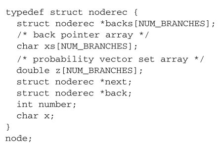
To describe the implementation of SPR pointer mesh updates in RAxML, we initially need to review the memory and data-structure organization for the single-gene case. The memory space required by standard likelihood implementations is dominated by the length and number of ancestral probability vectors. Thus, the memory requirements are of order Θ(n * m) where n is the number of taxa and m the number of distinct site patterns in the alignment. An unrooted phylogenetic tree for an alignment of dimensions n * m has n tips or leaves and n − 2 inner nodes, such that n − 2 ancestral vectors of length m are required. Note that, the computation of the vectors at the tips of the tree (leaf-vectors) is significantly less expensive and requires less memory than the computation of inner vectors (Tzeng, 2006).

In RAxML, only one ancestral probability vector per internal node, is allocated. This vector is relocated to one of the three outgoing branches of an internal node noderec *next (see data structure below) of the inner node that points towards the current virtual root. This concept is also called a view by Felsenstein (1981), because the ancestral likelihood vectors always maintain a rooted view of the tree towards the current position of the root. If the ancestral probability vector is already located at the correct outgoing branch (iff. the value of x == 1) it must not be recomputed. To move ancestral probability vectors among outgoing branches of an inner node, a cyclic list of three data structures of type node (one per outgoing branch struct noderec *back) is used (Fig. 3), which represents a single ancestral node of the tree. At all times, two of the entries for x in the cyclic list representing an inner node are set to x = 0;, whereas the remaining one is set to x = 1;. The actual probability vector data is then indexed via the node number number. Finally, the vector z[NUM_BRANCHES] contains the branch lengths for every partition that connects the present node in the cyclic list to the node that is addressed via the respective back pointer.

Using this type of data organization, when the virtual root is placed into a different part of the tree (for instance, to optimize a branch or when the tree topology has been altered), a certain number of ancestral vectors must be recomputed.

The above data-structure node can be extended as indicated below to accommodate the comprehensive tree topology t as well as the per-gene tree topologies as follows: we extend the data structure by an array of back-pointers backs that point to the neighboring nodes for each per-gene tree. Note that, the address of the back-pointer of partition 0 for instance might be located further away, that is, backs[0] == back does not necessarily hold. In addition, the array xs[NUM_BRANCHES] provides analogous information as x, but for each gene separately. By design, if a certain inner node represented by a linked cyclic list of three node structures, does not form part of a reduced tree for Gene i t|G_i, all respective entries are set to Null and 0, respectively: backs[i] = NULL;, xs[i] = 0;. If they do form part of the per-gene tree all three entries of backs[i] != NULL; and one of the xs[i] must be set to 1.

3.2 Computing a traversal on a fixed tree

To conduct a tree traversal on a fixed tree for optimizing model parameters and/or branch lengths, we initially place virtual roots for each gene separately. For each gene, we may just place the virtual root into the first taxon of the respective partition for which data is available. Given a comprehensive tree topology, we then recursively setup a per-gene pointer mesh by navigating through the comprehensive tree as described by Stamatakis and Ott (2008b). The key property of this pointer mesh at any ancestral node is that either all outgoing pointers for a specific partition are set to NULL or all outgoing pointers point to another node in the tree that contains data for the specific gene. That is, a node of the comprehensive tree either forms part of the per-gene subtree or not.

To compute the likelihood, optimize branch lengths and model parameters for the fixed comprehensive tree, we simply need to execute Felsenstein's pruning algorithm individually on every gene by using the respective pointer meshes and branch lengths induced by *backs[NUM_BRANCHES] and z[NUM_BRANCHES]. The dotted lines in Figure 2 indicate the reduced tree data structures given by the backs[] arrays (the traversal path for a subtree), while the straight line represents the overall tree topology as provided by the back pointers. To achieve the desired memory reduction for ancestral probability vectors (in contrast to the initial paper (Stamatakis and Ott, 2008b) where this was not implemented), for each gene we only assign as much memory as is required for the number of ancestral nodes contained in the gene-tree. Since we address ancestral vectors via the node number, this means that in the course of computations, per-gene trees are always represented by the same nodes in memory, that is, a node that once formed part of a gene tree will always from part of that gene tree.

The branch length optimization procedure works analogously, with the only difference that xs[NUM_BRANCHES] are also updated, since optimizing the branch lengths of a tree induces continuously re-rooting the tree at the branch to be optimized. Thus, one can easily use the above data structure to successively optimize the branches in every gene tree individually. For a more detailed description please refer to Stamatakis and Ott (2008b). Finally, it is important to note that, the speedups reported here are smaller than those reported previously (Stamatakis and Ott, 2008b) because of a bug in the branch length optimization convergence criterion under the standard model, that has been fixed in the latest release (v 7.2.6) of RAxML.

4 DYNAMIC MESHES

Given the prolegomena, we can now introduce the set of rules for per-gene pointer mesh updates that are required to conduct SPR moves on the above data structure. For this, we need to consider the pruning (removing a subtree at a specific branch of the comprehensive tree) and re-grafting (inserting the pruned subtree into branches of the tree) steps separately.

4.1 Subtree pruning

If we prune a subtree from a branch of the comprehensive tree as shown in Figure 4, we have to consider the following cases.

Fig. 4.

Pruning of a subtree.

Case 1: if the subtree to be pruned does not contain any data for Gene i, the induced gene-tree will be invariant with respect to any SPR moves of that subtree and hence the log likelihood LnL(t|G_i) will be invariant as well. Therefore, we just need to set a respective flag for Gene i and add the current likelihood for partition i to the likelihood of the other genes that may change because of the SPR move. We can check if the subtree does not contain data for Gene i by a simple recursive descent for partition i using the corresponding pointer mesh in that subtree.

Case 2: if the node to which the subtree is attached in the comprehensive tree forms part of a gene i, i.e. if all backs[i] are not set to NULL, we store the values of all three outgoing backs[i] pointers and remove the node from the per-gene pointer mesh.

Case 3: if the node to which the subtree is attached in the comprehensive tree does not form part of the gene tree i we proceed as follows: initially, we determine whether data for Gene i is contained in the left or right subtree rooted at the branch from which the subtree is pruned. If neither the left, nor the right subtree contain data for Gene i this means that the gene-tree for i is entirely contained in the subtree to be pruned. Therefore, we once again set a respective flag for Gene i that there is no work to do and store the current likelihood score for this partition. Otherwise, either the left, or the right subtree, or both subtrees will contain data for partition i. In the case that both subtrees of the pruning branch as well as the subtree to be pruned contain data, we connect the nodes in the left and right subtrees and prune the subtree. If only one of the two subtrees defined by the pruning branch contains data, this means that the subtree to be pruned is directly connected to a node in one of the two pruning branch subtrees.

In all cases where there is work to do, we always store the nodes that define the left and the right end of the branch (the pruning branch) from which the subtree is to be removed. Finally, after pruning the subtree the branch length of the pruning branch from which the subtree was removed is optimized via a Newton–Raphson procedure.

Once we have pruned the subtree and stored the required data, we can start re-inserting the pruned subtree into the remainder of the comprehensive tree.

4.2 Subtree regrafting

The SPR moves are also initially conducted on the comprehensive tree data structure. For each insertion branch in the comprehensive tree into which the candidate subtree shall be inserted, we once again conduct a case analysis to determine if the specific SPR move on the comprehensive tree also induces a change in the gene trees. For the cases described in Section 4.1 where the pruned subtree either contains all taxa of a gene or not a single taxon of a Gene i we are done. This is because the SPR move will not induce any changes to LnL(t|G_i). Thus, in this case, we simply add the stored likelihood of the gene to the overall likelihood we intend to compute.

In all other cases, the SPR move on the comprehensive tree may induce changes on the gene tree likelihoods. If we consider the insertion branch, i.e. the branch of the comprehensive tree into which the subtree shall be inserted, we once again need to determine recursively, if the left or the right subtree of the insertion branch contains molecular data for a partition i (Fig. 5).

Fig. 5.

Subtree insertion into a branch, where both the left and right subtrees contain data for a specific Gene i.

Case 1: if some nodes in the left and the right subtree of the insertion branch contain data for partition i as outlined in Figure 5, this means that the two subtrees must be connected by a branch of the partition, the partition insertion branch, into which the subtree shall be inserted. We obtain the per-gene insertion branch by recovering the two nodes that determine this branch via a recursive descent into the left and right subtree of the insertion branch in the comprehensive tree.

However, given that each gene tree contains at most as many ancestral nodes as the comprehensive tree, it may happen that the insertion branch for the subtree of partition i is identical (and hence the insertion likelihood is identical) for distinct insertion branches in the comprehensive tree as shown in Figure 6. Thus, the likelihood that is induced by repeatedly inserting the gene subtree i between the two nodes A and B that form a branch of the gene tree is identical. In other words, for the five subtree insertions of the comprehensive tree between nodes A and B the tree topology induced for the gene tree i is invariant. Thus, the likelihood score for insertions of subtree i between nodes A and B only needs to be computed once. To achieve computational savings, we therefore use a simple linked list to store and look up the gene tree insertion branch nodes/likelihood score triplets. For instance, at the first insertion of the subtree between Nodes A and B for gene i we will look up if the node pair A,B is stored in the respective list for partition i. If this is not the case, we will compute the likelihood score and store it in the list. For all successive insertions of the per-gene subtree between nodes A and B the lookup for partition i will be successful and we can hence simply re-use the per-gene likelihood score instead of re-computing it.

Fig. 6.

Outline of the optimization potential for subtree insertions into consecutive branches that have identical left and right subtrees for a specific Gene i.

Case 2: if only a node to the left or the right of the comprehensive insertion branch contains data for a partition i this means that a subtree for Gene i is located in one of the two subtrees but not both. In this case, we recursively descend into the subtree that contains the data until we find the first node that belongs to the gene tree i. If the node is not a leaf, it must be connected to another node in the same subtree of the comprehensive tree as shown in Figure 7. As before, we determine whether the candidate subtree has already been inserted into the respective branch of the gene tree by conducting a lookup in the aforementioned linked list. For example, in Figure 7 the insertion likelihood for Gene i is identical when the subtree is inserted into branches X,Y,Z of the comprehensive tree. If this is not the case, we insert the candidate subtree, compute its likelihood and add it to the likelihood scores of the remaining genes.

Fig. 7.

Insertion of a subtree into a branch at which only one of the two subtrees contains data for Gene i.

Finally, if either the left or the right subtree of the comprehensive insertion branch only contains a single taxon for Gene i this taxon represents the position from which the gene subtree was pruned. This case is already detected at the pruning stage and an appropriate flag is set that the likelihood for partition i will not need to be re-computed for any subtree insertion.

5 IMPLEMENTATION & EXPERIMENTAL SETUP

The pointer mesh update rules were implemented in the sequential SSE3-vectorized version (Berger and Stamatakis, 2009) of RAxML v7.2.5 (freely available at http://wwwkramer.in.tum.de/exelixis/software.html; mesh-based methods are implemented in file mesh.c).

To facilitate verification and comparison of the results, we implemented a simplified version of the lazy SPR move technique in RAxML (Stamatakis, 2006a).

The lazy SPR move technique of RAxML works as follows: Initially, the subtree to be rearranged (the candidate subtree) is pruned from the comprehensive tree topology. Then, only the branch from which the subtree was pruned is re-optimized via a Newton–Raphson procedure, as opposed to re-optimizing all branch lengths in the remaining tree. After this step, we can start inserting the candidate subtree into the branches of the remaining tree and compute the likelihood score for each insertion. When lazy SPR moves are used, we only re-optimize the three branch lengths that are adjacent to the insertion position of the candidate subtree, instead of re-optimizing all branches of the resulting tree. Thereby, we only obtain an approximate likelihood score instead of a ML score for each subtree rearrangement, that is, we conduct a lazy evaluation of SPR moves. The fast and slow lazy SPR moves implemented in RAxML differ in the way the three branch lengths adjacent to the subtree insertion position are optimized. Fast lazy SPR moves use an empirical best guess for the three branches, while slow lazy SPR moves deploy the Newton–Raphson procedure. Note that, other widely used ML-based inference programs such as PHYML v3.0 and GARLI also use variants of lazy SPR moves. The lazy SPR move technique is outlined in Figure 8.

Fig. 8.

Lazy SPR move technique of the standard RAxML algorithm.

The simplified version of the lazy SPR move technique implemented here, reads in a given starting tree, optimizes model parameters and branch lengths, and then applies only one cycle of lazy SPR moves to the tree with a rearrangement radius that is fixed to 10. One cycle of SPR moves means that every subtree of the comprehensive tree will be pruned and re-inserted into all neighboring branches of the pruning branch up to a distance of 10 nodes away from the original pruning position.

In addition, unlike the standard RAxML search mechanism the algorithm will not immediately keep SPR-generated topologies that yield an improvement, i.e., it only searches for the best lazy SPR move on the tree that was provided as input. The algorithm stores the best move on the comprehensive tree and will then write to file the comprehensive tree generated by the best SPR move. For verification purposes, this output tree can then be used to independently compute likelihood scores on the tree topologies obtained by the standard method and the fast mesh-based method we propose here.

The program will also print out the execution time required for model optimization, the execution time of one SPR cycle, and the overall execution time. The lazy SPR searches can be executed using fast lazy insertion and slow/thorough lazy insertions (Stamatakis, 2006a). The respective command lines are

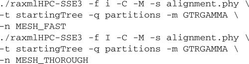
for the mesh-based approach and

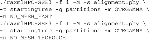
for the standard approach.

The inferences were conducted under the General Time Reversible (GTR) model of nucleotide substitution (Tavaré, 1986) and the WAG (Whelan and Goldman, 2001) amino acid substitution model for protein data. In all cases, we used the standard Γ model of rate heterogeneity (Yang, 1994).

The computational experiments were executed on a single core of an unloaded SUN x4600 multi-core machine with 32 cores and 64 GB RAM. The program was compiled with gcc v4.3.2 and the standard Makefile for the sequential SSE3 code that is distributed with the source files.

5.1 Datasets

We used six real world DNA and protein datasets containing 59 up to 37 831 taxa and six up to 1487 genes. The gappyness because of missing gene data ranged between 27% and 90%. Table 3 indicates the gappyness of the alignments used (not counting real alignment gaps). For ease of reference, we denote all datasets by dY_X where Y indicates the number of taxa and X the number of genes. Dataset d94_1487 is a protein alignment (Hejnol et al., 2009), all other datasets are DNA alignments. All datasets, partition files and starting trees, except for the unpublished dataset d37831_6, are available for download at http://wwwkramer.in.tum.de/exelixis/pointerMeshData.tar.bz2.

Table 3.

Gene-sampling induced gappyness and memory consumption of non-mesh based and mesh-based approach

Dataset	Gappyness	Memory nomesh	Memory mesh
d59_8	27.70%	25 MB	19 MB
d94_1487	81.31%	14.0 GB	2.8 GB
d128_34	28.30%	317 MB	234 MB
d404_11	69.15%	378 MB	125 MB
d2177_68	89.53%	9.0 GB	1.1 GB
d37831_6	75.41%	44.0 GB	14.0 GB

6 RESULTS

The recursive lookups to search for gene nodes in the pruning branch and insertion branch subtrees are implemented naïvely, by recursive descents into subtrees. While this is algorithmically not very elegant, the efficiency of this procedure is not critical because a profiling run using gprof on datasets d59_8 and d404_11 revealed that the recursive search procedures account for <1% of total execution time. On d37831_6 the contribution may be higher, but a profiling run could not be conducted because of excessive run-times and the significant slowdown associated with profiling.

In Table 1, we indicate the execution time speedups between the standard implementation and the mesh-based approach for model parameter optimization (denoted as Model optimization) as well as fast lazy (denoted as Fast SPR) and slow lazy SPR searches (denoted as Slow SPR). Overall, speedups for the fast lazy SPRs tend to be higher than for the thorough lazy SPRs, particularly for protein data.

Table 1.

Speedups of mesh-based likelihood approach versus standard approach

Dataset	Model optimization	Fast SPR	Slow SPR
d59_8	1.30	2.04	1.59
d94_1487	5.56	16.69	4.41
d126_34	1.34	1.79	1.80
d404_11	3.05	4.91	3.51
d2177_68	11.24	16.08	10.26
d37831_6	3.86	5.36	3.99

In Table 2, we provide the overall execution times in seconds (including file I/O, model optimization, and SPR searches) for the mesh-based and standard (denoted as NoMesh) likelihood function implementations using the fast and the more thorough lazy SPR moves.

Table 2.

Total execution times in seconds of mesh-based approach versus standard approach

Dataset	Fast mesh	Fast nomesh	Slow mesh	Slow nomesh
d59_8	21	32	74	114
d94_1487	7 493	77 960	92 573	408 794
d128_34	1 106	1 592	2 741	4 523
d404_11	159	597	597	2,066
d2177_68	7 395	87 320	15 455	164 168
d37831_6	31 597	130 776	94 497	367 139

In Table 3, we provide the gappyness of each dataset, i.e. the proportion of entirely missing data per gene over the entire alignment and the memory footprint for inferences under GTR+Γ and WAG+Γ for the mesh-based and standard approach. The memory savings are roughly proportional to the degree of gappyness.

Finally, in Table 4 we depict the likelihood scores of the trees computed independently by optimizing the likelihood score on the resulting SPR-modified trees obtained by the mesh-based and standard method. The scores on the trees were optimized using the mesh-based approach to save time, but for the smaller datasets we also conducted a tree evaluation using the standard approach. As already mentioned, likelihood scores may be slightly different if model parameters are optimized using the standard approach because of numerical deviations. It is interesting to observe that for thorough lazy SPR moves, the mesh-based approach yields slightly better likelihood scores on dataset d2177_68 and d94_1487. This can be attributed to numerical error propagation, because under the standard approach a significantly larger number of computations is conducted that may introduce rounding errors.

Table 4.

Log likelihoods of final trees generated by mesh and non-mesh based fast and slow SPR cycles

Dataset	Fast mesh	Fast nomesh	Slow mesh	Slow nomesh
d59_8	–50439.82	–50439.82	–50434.80	–50434.80
d94_1487	–5996718.37	–5996718.37	–5996650.63	–5996707.99
d128_34	–779459.01	–779459.01	–779446.71	–779446.71
d404_11	–151064.76	–151064.76	–151064.76	–151064.76
d2177_68	–2166752.48	–2166752.48	–2166237.10	–2166433.84
d37831_6	–5418619.45	–5418619.45	–5418648.55	–5418648.55

7 DISCUSSION

We have presented the first generally applicable rule set and an open source implementation for dynamically updating pointer meshes that represent per-gene subtrees induced by a comprehensive tree during SPR moves on phylogenomic alignments.

By deploying this rule set, we can significantly reduce the number of floating point operations required to compute the phylogenetic likelihood function and thereby accelerate likelihood-based tree searches by up to one order of magnitude. Perhaps more importantly, our method also allows for a memory footprint reduction that is proportional to the gappyness (proportion of missing data) of the alignment. Large and computationally challenging phylogenomic analyses under likelihood that would otherwise require supercomputers can now be conducted on a desktop computer. More importantly, the methods presented here can be applied to all likelihood-based (ML and Bayesian) programs for accelerating computations on typical phylogenomic alignments.

While we have demonstrated that we can achieve memory and time savings of one order of magnitude by deploying our rule set on datasets with a gappyness of ∼90%, the major challenge still lies ahead. Because of the increasing complexity in phylogenetics software, the main challenge will consist in supporting all search options of RAxML under all models (binary, DNA, secondary structure, multi-state, protein) both for the sequential as well as the parallel Pthreads-based version. In particular with respect to parallelization, we expect novel challenges in terms of handling load-balance among threads.

REFERENCES

- Berger SA, Stamatakis A. Proceedings of PBC09, Parallel Biocomputing Workshop. LNCS, Springer; 2009. Accuracy and performance of single versus double precision arithmetics for Maximum Likelihood Phylogeny Reconstruction. accepted for publication. Available at http://wwwkramer.in.tum.de/exelixis/pubs/PBC2009.pdf. [Google Scholar]
- Felsenstein J. Evolutionary trees from DNA sequences: a maximum likelihood approach. J. Mol. Evol. 1981;17:368–376. doi: 10.1007/BF01734359. [DOI] [PubMed] [Google Scholar]
- Goldman N, Yang Z. Introduction. statistical and computational challenges in molecular phylogenetics and evolution. Philos. Trans. R. Soc. B, Biol. Sci. 2008;363:3889. doi: 10.1098/rstb.2008.0182. [DOI] [PMC free article] [PubMed] [Google Scholar]
- Guindon S, Gascuel O. A simple, fast and accurate algorithm to estimate large phylogenies by Maximum Likelihood. Syst. Biol. 2003;52:696–704. doi: 10.1080/10635150390235520. [DOI] [PubMed] [Google Scholar]
- Hejnol A, et al. Rooting the bilaterian tree with scalable phylogenomic and supercomputing tools. Proc. R. Soc. B. 2009;276:4261–4270. doi: 10.1098/rspb.2009.0896. [DOI] [PMC free article] [PubMed] [Google Scholar]
- Lartillot N, et al. PhyloBayes. v2. 3. 2007 [Google Scholar]
- Pratas F, et al. Proceedings of the 2009 International Conference on Parallel Processing. Washington, DC: IEEE Computer Society; 2009. Fine-grain parallelism for the phylogenetic likelihood functions on Multi-cores, Cell/BE, and GPUs; pp. 9–17. [Google Scholar]
- Price MN, et al. Fasttree 2 - approximately maximum-likelihood trees for large alignments. PLoS ONE. 2010;5:e9490. doi: 10.1371/journal.pone.0009490. [DOI] [PMC free article] [PubMed] [Google Scholar]
- Ronquist F, Huelsenbeck J. MrBayes 3: Bayesian phylogenetic inference under mixed models. Bioinformatics. 2003;19:1572–1574. doi: 10.1093/bioinformatics/btg180. [DOI] [PubMed] [Google Scholar]
- Stamatakis A. RAxML-VI-HPC: maximum likelihood-based phylogenetic analyses with thousands of taxa and mixed models. Bioinformatics. 2006a;22:2688–2690. doi: 10.1093/bioinformatics/btl446. [DOI] [PubMed] [Google Scholar]
- Stamatakis A. Proceedings of IPDPS2006 HICOMB Workshop, Proceedings on CD. Rhodos, Greece: IEEE; 2006b. Phylogenetic models of Rate Heterogeneity: A High Performance Computing Perspective. [Google Scholar]
- Stamatakis A, Ott M. Exploiting Fine-Grained Parallelism in the Phylogenetic Likelihood Function with MPI, Pthreads, and OpenMP: A Performance Study. In: Chetty M, Ngom A, Ahmad S, editors. Partition Recognition for Bioinformatics. Vol. 5265. Berlin/Heidelberg: Springer; 2008a. pp. 424–435. of Lecture Notes in Computer Science. [Google Scholar]
- Stamatakis A, Ott M. Efficient computation of the phylogenetic likelihood function on multi-gene alignments and multi-core architectures. Philos. Trans. R. Soc. B, Biol. Sci. 2008b;363:3977–3984. doi: 10.1098/rstb.2008.0163. [DOI] [PMC free article] [PubMed] [Google Scholar]
- Suchard M, Rambaut A. Many-core algorithms for statistical phylogenetics. Bioinformatics. 2009;25:1370. doi: 10.1093/bioinformatics/btp244. [DOI] [PMC free article] [PubMed] [Google Scholar]
- Tavaré S. Some Mathematical Questions in Biology-DNA Sequence Analysis. Vol. 17. Providence, RI: American Mathematical Society; 1986. Some probabilistic and statistical problems in the analysis of DNA sequences; pp. 57–86. [Google Scholar]
- Tzeng C.-W, editor. Advances in Computers. USA: Elsevier; 2006. [Google Scholar]
- Whelan S, Goldman N. A general empirical model of protein evolution derived from multiple protein families using a maximum-likelihood approach. Mol. Biol. Evol. 2001;18:691–699. doi: 10.1093/oxfordjournals.molbev.a003851. [DOI] [PubMed] [Google Scholar]
- Yang Z. Maximum likelihood phylogenetic estimation from DNA sequences with variable rates over sites. J. Mol. Evol. 1994;39:306–314. doi: 10.1007/BF00160154. [DOI] [PubMed] [Google Scholar]
- Zwickl D. PhD Thesis. Austin: University of Texas; 2006. Genetic Algorithm Approaches for the Phylogenetic Analysis of Large Biological Sequence Datasets under the Maximum Likelihood Criterion. [Google Scholar]