Quantifying the distribution of probes between subcellular locations using unsupervised pattern unmixing

Abstract

Motivation: Proteins exhibit complex subcellular distributions, which may include localizing in more than one organelle and varying in location depending on the cell physiology. Estimating the amount of protein distributed in each subcellular location is essential for quantitative understanding and modeling of protein dynamics and how they affect cell behaviors. We have previously described automated methods using fluorescent microscope images to determine the fractions of protein fluorescence in various subcellular locations when the basic locations in which a protein can be present are known. As this set of basic locations may be unknown (especially for studies on a proteome-wide scale), we here describe unsupervised methods to identify the fundamental patterns from images of mixed patterns and estimate the fractional composition of them.

Methods: We developed two approaches to the problem, both based on identifying types of objects present in images and representing patterns by frequencies of those object types. One is a basis pursuit method (which is based on a linear mixture model), and the other is based on latent Dirichlet allocation (LDA). For testing both approaches, we used images previously acquired for testing supervised unmixing methods. These images were of cells labeled with various combinations of two organelle-specific probes that had the same fluorescent properties to simulate mixed patterns of subcellular location.

Results: We achieved 0.80 and 0.91 correlation between estimated and underlying fractions of the two probes (fundamental patterns) with basis pursuit and LDA approaches, respectively, indicating that our methods can unmix the complex subcellular distribution with reasonably high accuracy.

Availability: http://murphylab.web.cmu.edu/software

Contact: murphy@cmu.edu

1 INTRODUCTION

To investigate the subcellular localization of proteins at a proteome-wide scale, we need to be able to characterize all observed patterns. Identification of subcellular localization patterns from fluorescence images using supervised machine learning methods has become an established method, with excellent results in its field of application. However, this method is, by design, limited to hard assignments to classes predefined by the researcher. Some researchers have explored using unsupervised learning technologies (García Osuna et al., 2007; Hamilton et al., 2009), which do not require the researcher to specify classes. These methods still result in each protein being assigned a single label.

However, not all proteins can be thus characterized. In particular, there are many proteins that exhibit ‘mixed patterns’, i.e. patterns that are composed of more than one location. For example, while some proteins locate in the nucleus and others locate in the endoplasmic reticulum, there is a third group that locates in both of these locations. A simple class assignment does not adequately represent the relationship between these three possibilities. One alternative is to assign multiple labels to a single pattern. In one large-scale study of the yeast proteome, a third of proteins were annotated with multiple locations, which demonstrates that this is not a problem confined to ‘special case’ proteins (Chen et al., 2007; Huh et al., 2003). However, this approach fails to quantify the contribution of each element and shows the need for a system that directly models the mixture phenomenon.

We have previously presented some methods that address this pattern unmixing problem in a supervised setting: given images of fundamental patterns (e.g. nuclear and endoplasmic reticulum in the above example) and mixed images, map mixed images into a set of coefficients, one for each fundamental pattern (Peng et al., 2010; Zhao et al., 2005). These methods were observed to perform well on both synthetic and real data in recovering the underlying mixture coefficients (which had been kept hidden from the algorithm).

However, the supervised approach still requires the researcher to specify the fundamental patterns of which other patterns are composed. For example, for the quantitative analysis of translocation experiments as a function of time or drug concentration, the extreme points could be easily identified as the patterns of interest. However, they are still inapplicable to proteome-wide studies where it would be a difficult (and perhaps impossible) task to identify all fundamental patterns that are present. We note that the set of fundamental patterns that can be identified depends both on the specific cell type and the technology used for imaging, high-resolution confocal microscopes being able to distinguish patterns that lower resolution systems cannot.

Therefore, it is necessary to tackle the unsupervised pattern unmixing problem: given a large collection of images, where none has been tagged as being a representative of a fundamental pattern, map all images into a set of mixture coefficients automatically derived from the data.

In this article, we present and compare methods to address this problem using a test dataset previously created to test supervised unmixing methods (Peng et al., 2010).

2 METHODS

2.1 Object typing

2.1.1 Overview

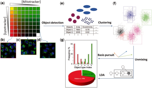
All the methods developed for this problem so far are based on a bag of objects model, where an image is interpreted as a collection of regions of above-background fluorescence. Each object is then characterized by a small set of object features, and objects are clustered into groups (object types). Patterns are then defined as distributions over these groups. This is illustrated in Figure 1.

Fig. 1.

Overview of unmixing methods. (a) The algorithms use a collection of images as input in which various concentrations of two probes are present (the concentrations of the Mitotracker and Lysotracker probes are shown by increasing intensity of red and green, respectively). Example images are shown from wells containing only Mitotracker (b), only Lysotracker (c) and a mixture of the two probes (d). (e) Objects with different size and shapes are extracted and object features are calculated. (f) Objects are clustered into groups in feature space, shown with different colors. (g) Fundamental patterns are identified and the fractions they contribute to each image are estimated.

The intuition is to capture patterns such as the fact that lysosomes are small mostly circular objects, while mitochondria consist of stringy objects. The methods need to be robust to stochastic variation, however, as mitochondrial patterns are also observed to contain circular objects and agglomerations of lysosomes may appear as a single stringy object. In fact, the algorithms need to capture not only the fact that mitochondrial patterns are composed of stringy objects, but also that the proportions of different types of objects are present in statistically different proportions.

2.1.2 Image preprocessing and segmentation

Images are first preprocessed to remove uneven illumination. The illumination bias is estimated by fitting a plane to the average pixel intensity at each location across the whole collection of images. Every image pixel is then divided by this illumination estimate to regularize across the whole image.

Images are segmented by using the model-based method of Lin et al. (2003) on the nuclear channel, which was previously found to give the best results for images in the unmixing test dataset (Coelho et al., 2009). The segmentation is extended to the whole field by using the watershed method with the segmented nuclei as seeds.

2.1.3 Object detection

In our previous supervised unmixing work, objects were simply defined as contiguous pixel regions above a global threshold. In the work described here, we use both a global threshold, using the Ridler–Calvard method (Ridler and Calvard, 1978), and a local threshold, the mean pixel value of a 15 × 15 window centered at the pixel. We have found that the global threshold achieves a good separation of the general cell areas from the background, while, inside those regions, local thresholding is better at capturing detail.

Objects that are smaller than 5 pixels are filtered out.

2.1.4 Object features

Each object is characterized by a set of features, previously defined as SOF1 (subcellular object features 1). This is a combination of morphological features for describing the shape and size of the object and features which capture the relationship to the nuclear marker (Zhao et al., 2005):

1. Size (in pixels) of the object.

2. Distance of object center of fluorescence to DNA center of fluorescence.

3. Fraction of object that overlaps with DNA.

4. Eccentricity of object hull.

5. Euler number of object.

6. Shape factor of convex hull.

7. Size of object skeleton.

8. Fraction of overlap between object convex hull and object.

9. Fraction of binary object that is skeleton.

10. Fraction of fluorescence contained in skeleton.

11. Fraction of binary object that constitutes branch points in the skeleton.

2.1.5 Object clustering

In order to be able to reason about object types, objects are clustered into groups using k-means on the z-scored feature space. Multiple values of k are tried and the one resulting in the lowest BIC (Bayesian information criterion) score is selected.

Based on this clustering, each object can be assigned a numerical identifier, its cluster index, which serves as its type.

After this step, the algorithms diverge in how they handle the cluster indices.

2.2 Basis pursuit

In this model, each image is represented by a vector x⁽ⁱ⁾ such that entry x⁽ⁱ⁾_ℓ represents the fraction of objects in condition i that have type ℓ (if there are multiple images for the same condition, a common situation, they are counted together). We have one vector per input condition (i.e. i = 1,…, C, where C is the number of conditions), and the size of this vector is the number of clusters that was automatically identified in the clustering step (i.e. ℓ = 1,…, k).

Using fractions instead of the direct object counts normalizes for the different number of cells in each image and different cell sizes.

In this model, bases (fundamental patterns) are represented as a set of vectors in the same space and a mixture is defined by a set of coefficients α_j for each b^(j) (j = 1,…, B, where B is the number of basis vectors, and each b^(j) is of the same dimension as the x⁽ⁱ⁾s):

(1)

where ε⁽ⁱ⁾ encapsulates both the stochastic nature of the mixing process and the measurement noise.

Given a set of observations, the task is to identify the bases b^(j) and coefficients α⁽ⁱ⁾, which minimize the squared norm of the error terms ∑_i‖ε⁽ⁱ⁾‖².

Without additional constraints, principal component analysis (PCA) is the simplest solution to this problem. However, this is unsatisfactory as it could result in negative mixtures, which are not meaningful. Independent component analysis (ICA) suffers from the same problem. Therefore, we add a non-negativity constraint on the vector α and use non-negative matrix factorization (NNMF) possibly with sparsity constraints to solve the problem (Hoyer et al., 2004; Lee and Seung, 1999).

An additional constraint can be helpful to obtain more meaningful results: require the basis vectors to be members of the input dataset (i.e. for all j, there is some i, such that b^(j) = x⁽ⁱ⁾). This condition, which encapsulates the expectation that the input dataset is large enough to contain both fundamental and mixed patterns, requires a search method.

Some preliminary results showed that this model was still too sensitive to the trend, i.e. to the average value of x_i,j across the dataset (data not shown). If one basis vector was allocated to handle this trend, good fits were obtained but poor interpretability. We found that removing the mean from the data led to more meaningful results. In this detrended dataset, may take negative values, but the mixing coefficients α_i,j are still constrained to be non-negative.

Thus, the final optimization problem is:

(2)

(3)

(4)

Subject to the constraint, that for all j, there exists an i, such that b^(j) = x⁽ⁱ⁾. In order to find the best basis, we resort to simulated annealing as an optimization method. In this class of methods, the number of fundamental patterns B must be prespecified by the user.

PCA and ICA were also performed on detrended data, but NNMF could not be (as the detrended data contains negative numbers, it cannot be the product of two positive matrices). Before applying NNMF, we therefore removed very frequent objects (those that appeared in more than 90% of the images). The intuition is that very frequent objects also correspond to the background.

2.3 Latent Dirichlet allocation

Topic modeling in text using latent Dirichlet allocation (LDA) is a popular technique to solve an analogous class of problems (Blei et al., 2003). In this framework, documents are seen as simple ‘bags of words’ and topics are distributions over words. Observed bags of words can be generated by choosing mixture coefficients for topics followed by a generation of words according to: pick a topic from which to generate, then pick a word from that topic.

In our setting, we view object classes as visual words over which to run LDA. This is similar to work by other researchers in computer vision which use keypoints to define visual words (Csurka et al., 2004; Philbin et al., 2008; Zhu et al., 2009).

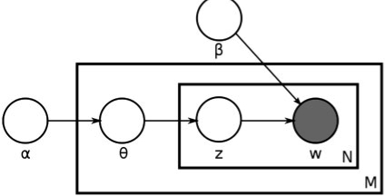
The process of generating objects in images to represent mixtures of multiple fundamental patterns follows the Bayesian network in Figure 2. The generative process is as follows: for each of M images, a mixture θ_i is first sampled (conditioned on the hyper-parameter α). θ_i is a vector of fractions of the fundamental pattern distributions b. N_i objects are sampled for each image in two steps: select a basis pattern according to tθ_i and then an object is sampled from the corresponding object type distribution.

Fig. 2.

LDA for unmixing. α represents the prior on the topics, θ is the topic mixture parameter (one for each of M images), z represents the particular object topic which is combined with β, the topic distributions to generate an object of type w.

To invert this generative process, we used the variational EM algorithm of Blei et al. (2003) to estimate the model parameters of fundamental patterns β and mixture fractions θ. It should be noted that this is an approximation approach liable to getting trapped in local maxima and returning non-optimal results. Therefore, we ran the algorithm multiple times with different random initializations and chose the one with the highest log-likelihood.

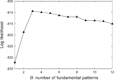
We choose the number of fundamental patterns B to maximize the log likelihood on a held-out dataset (using cross-validation to obtain more accurate estimate).

3 RESULTS

3.1 Dataset

In order to validate the algorithms, we used a test set that was built to evaluate pattern unmixing algorithms (Peng et al., 2010).

In this dataset, u2os cells were exposed to different concentrations of two fluorescent probes with differing localization profiles (mitochondrial and lysosomal) but similar fluorescence. The probes were image using the same fluorescence filter and therefore could not be distinguished. This simulates the situation in which a fluorophore is present in two different locations. For each probe, eight concentrations were used, for a total of 64 combinations.

In parallel to the marker image, a nuclear marker was imaged to serve as a reference point.

3.2 Computation time

Most of the computation time is dominated by segmenting the images (∼30 s per image in our implementation) and computing features (∼10 s per image). However, this is an embarrassingly parallel problem and can be computed on multiple machines simultaneously. The clustering takes increasing time for different numbers of clusters, but we limited each clustering run to ∼1 h (while relying on multiple initialization as a guard against local minima). Again, we note that the runs for multiple k can easily be run in parallel. Both basis pursuit and LDA then take only on the order of minutes to run.

3.3 Basis pursuit

We measured how well the identified coefficients α⁽ⁱ⁾_j correlated with the underlying fractions, which were estimated as linearly proportional to the ratio of the relative concentration of the mitochondrial probe to the sum of the relative concentration of the mitochondrial and lysosomal probes (relative concentration is defined as fraction of the maximum subsaturating concentration).

Using PCA, the correlation coefficient between predicted fractions and the underlying relative concentrations was 0.20. NNMF performed better on this metric, achieving a correlation coefficient of 0.65. Independent component analysis performed very poorly, returning correlations on the order of less than 0.10. This is not unexpected as the independence assumptions that underly ICA fail to hold even as an approximation.

However, we are also interested in having the basis vectors line up with the underlying fundamental patterns and, in this regard, NNMF performs poorly. One of the patterns corresponded roughly to the total concentration and they did not align well with the fundamental patterns in the data (data not shown).

The fully constrained basis pursuit algorithm performed better. It achieved a 0.80 correlation with the underlying relative concentration. It identified as a basis a vector that has the maximal concentration of the mitochondrial probe (and some lysosomal probe, at a relative concentration of 19%) and another that consists of the maximal concentration of the lysosomal probe and 20% mitochondrial probe. Table 1 shows that the identified pattern 0 matches the mitochondrial probe, while pattern 1 matches the lysosomal probe.

Table 1.

Unmixed coefficients for images of fundamental patterns and mixed samples using basis pursuit with B = 2

	Mitochondrial (%)	Lysosomal (%)
Pattern 0	99	18
Pattern 1	1	82

For the two fundamental patterns, we display the average coefficient for the inferred fundamental patterns.

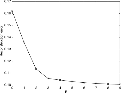
The results above were obtained by specifying B = 2 as an input to the algorithm. For different values of B, we obtain decreasing reconstruction error as plotted in Figure 3. As it is clear in this figure, most of the contribution to the reconstruction comes from the first two or three vectors. Therefore, we can expect that a researcher would be able to estimate B = 2 or B = 3.

Fig. 3.

Average squared reconstruction error as a function of the number of patterns B for basis pursuit. This is the value of ∑_i ‖ε‖² in (2). For B = 0, we show the total variance, i.e.

3.4 LDA

To estimate the number of fundamental patterns using the LDA approach, we measured the log likelihood of the dataset for different numbers of bases using cross-validation. The results are shown in Figure 4. We can see that the best result is obtained for B = 3, although the underlying dataset only has two fundamental patterns.

Fig. 4.

Log likelihood as a function of the number of fundamental patterns.

Table 2 shows the average coefficients inferred for pure pattern inputs after the algorithm had been applied on the whole dataset. Pattern 1 obviously corresponds to the lysosomal component, while pattern 2 corresponds to the mitochondrial component. Pattern 0 appears to be a ‘non-significant’ pattern capturing the new object types arising in the mixture patterns. The overall correlation coefficient is 0.95 with pattern 0 removed.

Table 2.

Unmixed coefficients for fundamental patterns and mixed samples for the discovered patterns (using LDA method)

	Mitochondrial (%)	Lysosomal (%)
Pattern 0	0.0	0.0
Pattern 1	8.8	99.9
Pattern 2	91.2	0.1

For the two fundamental patterns, we display the average coefficient for the three discovered fundamental patterns.

Using the LDA approach with B = 2, which is the ground truth, the overall correlation coefficient between estimated and actual pattern fractions was found to be 0.91.

3.5 Comparisons

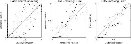
Figure 5 shows the results of one inferred fraction as a function of the underlying concentrations (the plots for the other fraction, not shown, are, of course, symmetric as they sum to 1). Figure 6 plots all the estimates in a single plot as a function of the underlying concentration fractions.

Fig. 5.

Comparison of results for different unmixing methods. The inferred fraction of pattern 1 is displayed as different intensities of gray (black corresponding to pure pattern 1). The design matrix, which was kept hidden from the algorithms is shown on the top left, for comparison; the other three panels are results of computation.

Fig. 6.

Estimated concentration as a function of the underlying relative probe concentration. Perfect result would be along the dashed diagonal. In LDA unmixing with 3 fundamental patterns, fractions of the two major patterns are normalized and plotted over ground-truth.

4 DISCUSSION

We have described two approaches for performing unsupervised unmixing of subcellular location patterns, and demonstrated good performance with both on a test dataset acquired by high-throughput microscopy and previously used for testing supervised methods.

In our supervised work, we had presented two methods, one based on a linear mixture, whose adaptation to the unsupervised case results in the basis pursuit method described here, and another based on multinomial mixtures, which results in the LDA model.

The newer LDA model led to slightly better results than the basis pursuit method. This model has the apparent disadvantage that it does not return examples of the underlying patterns, which could potentially make interpretation harder. However, we observed that this was, empirically, not a major issue as the identified bases were indeed well aligned with the underlying (hidden) concentrations as opposed to forming a complex mixture with a difficult interpretation.

The methods are comparable in terms of computational cost as it is the image processing, feature computation and, particularly, the k-means clustering that has the highest cost (the clustering is done over objects and even this evaluation set of ∼12 K images resulted in ∼750 K objects). Once the clustering is done, both algorithms are very fast. Therefore, in their current forms, the LDA algorithm is superior.

It is notable that both unsupervised methods led to higher correlation with the underlying coefficients than the supervised methods. A possible cause of this is the appearance of new object types in the mixture patterns. Under the unsupervised framework, with massive clustering, these objects might be assigned labels different from the ones of the fundamental patterns, while in the supervised version they are forced to be one of the object types present in the fundamental patterns. To prove this conjecture, we assumed that such new types of objects really exist and applied the outlier removal technique of Peng et al. (2010) to perform supervised unmixing again, in the hope of removing the influence of these objects. The correlations increased to 0.91 and 0.88 with linear and multinomial unmixing approaches, respectively, which are comparable with the unsupervised results.

Based on the results presented here, we plan to apply the unsupervised unmixing methods to large-scale image collections with the goal of identifying both the set of all fundamental patterns and of quantitating for the first time the fraction of all proteins that are present in each.

REFERENCES

- Blei DM, et al. Latent Dirichlet allocation. J. Mach. Learn. Res. 2003;3:993–1022. [Google Scholar]
- Chen S.-C, et al. Automated image analysis of protein localization in budding yeast. Bioinformatics. 2007;23:i66–i71. doi: 10.1093/bioinformatics/btm206. [DOI] [PubMed] [Google Scholar]
- Coelho LP, et al. Proceedings of the 2009 IEEE International Symposium on Biomedical Imaging. Piscataway, NJ, USA: IEEE; 2009. Nuclear segmentation in microscope cell images: a hand-segmented dataset and comparison of algorithms; pp. 518–521. [DOI] [PMC free article] [PubMed] [Google Scholar]
- Csurka G, et al. Workshop on Statistical Learning in Computer Vision. Prague, Czech Republic: ECCV; 2004. Visual categorization with bags of keypoints; pp. 1–22. [Google Scholar]
- García Osuna E, et al. Large-scale automated analysis of location patterns in randomly tagged 3T3 cells. Ann. Biomed. Eng. 2007;35:1081–1087. doi: 10.1007/s10439-007-9254-5. [DOI] [PMC free article] [PubMed] [Google Scholar]
- Hamilton NA, et al. Statistical and visual differentiation of subcellular imaging. BMC Bioinformatics. 2009;10:94. doi: 10.1186/1471-2105-10-94. [DOI] [PMC free article] [PubMed] [Google Scholar]
- Hoyer PO. Non-negative matrix factorization with sparseness constraints. J. Mach. Learn. Res. 2004;5:1457–1469. [Google Scholar]
- Huh W.-K, et al. Global analysis of protein localization in budding yeast. Nature. 2003;425:686–691. doi: 10.1038/nature02026. [DOI] [PubMed] [Google Scholar]
- Lee DD, Seung HS. Learning the parts of objects by non-negative matrix factorization. Nature. 1999;401:788–791. doi: 10.1038/44565. [DOI] [PubMed] [Google Scholar]
- Lin G, et al. A hybrid 3D watershed algorithm incorporating gradient cues and object models for automatic segmentation of nuclei in confocal image stacks. Cytometry A. 2003;56A:23–36. doi: 10.1002/cyto.a.10079. [DOI] [PubMed] [Google Scholar]
- Peng T, et al. Determining the distribution of probes between different subcellular locations through automated unmixing of subcellular patterns. Proc. Natl Acad. Sci. USA. 2010;107:2944–2949. doi: 10.1073/pnas.0912090107. [DOI] [PMC free article] [PubMed] [Google Scholar]
- Philbin J, et al. Proceedings of the British Machine Vision Conference. Leeds, UK: 2008. Geometric LDA: a generative model for particular object discovery. [Google Scholar]
- Ridler T, Calvard S. Picture thresholding using an iterative selection method. IEEE Trans. Syst. Man Cybernet. 1978;8:630–632. [Google Scholar]
- Zhao T, et al. Object type recognition for automated analysis of protein subcellular location. IEEE Trans. Image Process. 2005;14:1351–1359. doi: 10.1109/tip.2005.852456. [DOI] [PMC free article] [PubMed] [Google Scholar]
- Zhu L, et al. Unsupervised learning of probabilistic grammar-Markov models for object categories. IEEE Trans. Pattern Anal. Mach. Intell. 2009;31:114–128. doi: 10.1109/TPAMI.2008.67. [DOI] [PubMed] [Google Scholar]