Efficient identification of identical-by-descent status in pedigrees with many untyped individuals

Abstract

Motivation: Inference of identical-by-descent (IBD) probabilities is the key in family-based linkage analysis. Using high-density single nucleotide polymorphism (SNP) markers, one can almost always infer haplotype configurations of each member in a family given all individuals being typed. Consequently, the IBD status can be obtained directly from haplotype configurations. However, in reality, many family members are not typed due to practical reasons. The problem of IBD/haplotype inference is much harder when treating untyped individuals as missing.

Results: We present a novel hidden Markov model (HMM) approach to infer the IBD status in a pedigree with many untyped members using high-density SNP markers. We introduce the concept of inheritance-generating function, defined for any pair of alleles in a descent graph based on a pedigree structure. We derive a recursive formula for efficient calculation of the inheritance-generating function. By aggregating all possible inheritance patterns via an explicit representation of the number and lengths of all possible paths between two alleles, the inheritance-generating function provides a convenient way to theoretically derive the transition probabilities of the HMM. We further extend the basic HMM to incorporate population linkage disequilibrium (LD). Pedigree-wise IBD sharing can be constructed based on pair-wise IBD relationships. Compared with traditional approaches for linkage analysis, our new model can efficiently infer IBD status without enumerating all possible genotypes and transmission patterns of untyped members in a family. Our approach can be reliably applied on large pedigrees with many untyped members, and the inferred IBD status can be used for non-parametric genome-wide linkage analysis.

Availability: The algorithm is implemented in Matlab and is freely available upon request.

Contact: jingli@cwru.edu

Supplementary information: Supplementary data are available on Bioinformatics online.

1 INTRODUCTION

As one important type of gene mapping approach, family-based linkage analysis has shown tremendous success in identifying genes underlying Mendelian diseases. With the development of new genotyping technologies, there have been two distinct features arising in new datasets: both the number of genetic markers, mostly single nucleotide polymorphisms (SNPs), and the number of untyped individuals within a pedigree have increased drastically. Traditional linkage methods are exponential either in terms of the number of markers [i.e. Elston–Stewart i.e. Elston and Stewart, 1971)], or in terms of the size of a pedigree [Lander–Green (Lander and Green, 1987)], therefore cannot efficiently deal with new data. The problem is much harder for families with many untyped individuals. Even later approaches (Abecasis et al., 2002; Geiger et al., 2009; Gudbjartsson et al., 2005; Kruglyak et al., 1996; Sobel and Lange, 1996) relying on heuristic search or using various search space reduction techniques cannot solve the problem. Furthermore, for tightly linked markers, the original assumption of linkage equilibrium between markers does not hold anymore. (Abecasis and Wigginton, 2005) address this problem by partitioning a chromosome into small segments, and assume that there is no recombination within each segment and SNPs in different segments are in linkage equilibrium. However, by uniformly partitioning chromosomes into segments with a fixed segment length, their approach cannot handle segments with recombinations. In addition, they basically implement the Lander-Green algorithm (Lander and Green, 1987), which enumerates all inheritance patterns; therefore, their approach cannot handle large pedigrees. Keith et al. (2008) also address linkage disequilibrium (LD) for tightly liked markers by modeling founder haplotypes as a Markov chain. However, their method is mainly for nuclear family data with two offsprings. Recently, we have demonstrated that with high-density SNP data, (i) we can infer recombination breakpoints with high precision (Li et al., 2010); (ii) our algorithm (Li and Li, 2009) can efficiently infer haplotypes and inheritance patterns for large pedigrees; and (iii) in most cases, inheritance can be uniquely determined for large pedigrees with large number of SNPs. Experimental results show that our approach is highly efficient and can also tolerate high missing rates. However, if there are individuals in the pedigree that are completely untyped, our approach still needs to enumerate all transmission patterns and genotypes involving these untyped individuals, which may end up searching an exponentially large solution space.

In this article, we address the key problem in linkage analysis using high-density SNPs and large pedigrees with many untyped members: IBD inference between any pair of typed members within a pedigree, by proposing a novel hidden Markov model (HMM) based approach. Our approach is fundamentally different from the Lander–Green algorithm, although both are based on HMMs. Lander–Green algorithm only models the parent–child relationship and it has to take into account every possible transmission pattern between a parent–child pair. Instead, our approach can directly model relationships between any pair of relatives. In our model, the hidden states are the IBD number between the pair at each locus and the observable data are the numbers of alleles that are identical-by-state (IBS) between the pair. Unlike the Lander–Green algorithm, the probability of identical-by-discent (IBD) change between two markers for a given pair not only depends on the marker interval distance, but also depends on the type of relationship of the pair. More precisely, the transition probabilities depend on all possible cases that how recombination events might occur between the two markers when the pair inherits their genes from their common ancestors within the pedigree. To derive the transition probabilities between any types of relationships, we introduce the inheritance-generating function, which can conveniently aggregate all possible inheritance patterns between their common ancestors and this pair of individuals. Actually, our definition of the inheritance-generating function can explicitly list the number of all possible inheritance paths and their lengths between a pair of alleles. We also propose an efficient recursive approach to calculate the function. The transition probabilities can then be theoretically derived based on the number and lengths of all inheritance paths. Emission probabilities can be derived based on their definitions. They only depend on population allele frequencies and genotyping error rates, but do not depend on the type of relationship between a pair. We first define our HMM for a pair of alleles. Based on this basic model, we build the model for a pair of individuals. We further extend the model to incorporate population LD or background sharing beyond a pedigree. Finally, pedigree-wise IBD sharing can be constructed based on pairwise IBD relationships. Compared with traditional approaches for linkage analysis (i.e. Elston–Stewart and Lander–Green algorithms), our algorithm is essentially quadratic in terms of the number of typed individuals and linear in terms of the number of markers. More importantly, our new model can efficiently infer IBD status without enumerating all possible genotypes and transmission patterns of untyped members in a family. Given the fact that most existing family data using high-density SNP chips consist of many untyped individuals, our approach provides an efficient alternative to perform genome-wide linkage analysis.

We evaluate our approach using small nuclear families, large multi-generation pedigrees as well as simulated data. Experimental results show that for siblings with untyped parents, which corresponds to a saving of 50% of total genotyping costs, our approach has successfully recovered >90% of IBD changing points (i.e. recombination breakpoints) with <5% false positives. We also construct the IBD sharing map of seven typed members in a pedigree of size 15. Simulation using this pedigree structure shows that for different types of pairwise relationships, our approach can recover 84.0–87.7% IBD changing points with high precision, while at the same time, keeping the false positive rate low (4.2–6.8%). In experiments on two other big pedigrees (size 22 and 23), our method maintains a locus-by-locus IBD inference error rate <1%. Comparisons with MERLIN (Abecasis et al., 2002) show that our algorithm is both more accurate and more efficient in identifying IBD sharing.

2 METHODS

The main purpose of the proposed method is to infer the IBD sharing status between any pair of genotyped individuals within a pedigree without enumerating the genotypes of their untyped ancestors. We achieve this goal by building an HMM model with the IBS sharing numbers between two individuals as observed data and their IBD sharing numbers as hidden states. To derive our model, we first introduce the concept of descent graph and define an inheritance-generating function between a pair of alleles in a descent graph. Then we build a basic HMM for a pair of alleles with the transition probabilities represented by the inheritance-generating function. We then derive a recursive formula, by taking advantage of the pedigree structure, to efficiently calculate the inheritance-generating function. The HMM for a pair of individuals can be constructed by assuming the independence between two homologous chromosomes within an individual. We further extend the HMM to handle LD by incorporating IBD sharing at the population level. Finally, IBD sharing among all typed members within a pedigree can be constructed based on pairwise IBD sharing.

2.1 Descent graph and inheritance-generating function

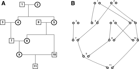
A descent graph (Sobel and Lange, 1996) of a pedigree consists of both the paternal and maternal allele of each individual as its vertices, and one link between each parent–child pair as its edges. Each edge specifies which of the two alleles of a parent is transmitted to a child. A descent graph illustrates one possible inheritance pattern within a pedigree, and by definition, it does not include genotype information. Figure 1 shows a pedigree and one of its many possible descent graphs. For any two nodes (i.e. two alleles) a and b in a descent graph, an inheritance path, denoted as p^a,b, is a simple undirected path that links a and b. It is easy to see that two alleles are IBD (descend from the same ancestral allele) if and only if there is an inheritance path between them. For example, in Figure 1, there is an inheritance path (dashed red line) between the paternal and maternal alleles of individual 11, which indicates that the two alleles are the copies of the same allele of their common ancestor (in this case, the paternal allele of member 2). As a descent graph is a realization of one particular inheritance pattern in a pedigree, for any two alleles, there is at most one inheritance path.

Fig. 1.

(A) a pedigree structure, drawn in a conventional way. (B) one of its many possible descent graphs. Each individual has two nodes, representing paternal and maternal alleles. An edge in the descent graph indicates which of the two alleles in a parent is transmitted to a child.

For any two alleles a and b in a pedigree at a SNP site, we define an inheritance-generating function:

where λ_ℓ is the number of all possible inheritance paths of length ℓ between a and b. Notice that there are only finite number of descent graphs for a given pedigree; therefore, there are only finite number of inheritance paths between two alleles and the summation only has finite number of terms. The generating function actually explicitly lists the numbers of paths of any lengths over all possible descent graphs of a pedigree. For simplicity, we drop the subscripts a and b in θ_a,b(h) when there is no ambiguity.

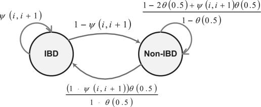
2.2 HMM for a pair of alleles

The structure of the two-state HMM for a pair of alleles is illustrated in Figure 2, with only transition probabilities labeled. Notice that this is actually a linear chain that generates a pair of haplotypes. We first derive transition probabilities using the generating function defined above. Then we will briefly discuss the derivation of emission probabilities. The transition probability from the state IBD to itself (Fig. 2) basically means that if two alleles a_i and b_i at locus i are IBD, what is the probability that two alleles a_i+1 and b_i+1 at locus i+1 on the same haplotypes are IBD. We denote this probability as . Given a_i and b_i are IBD, there may be many possible inheritance paths from different descent graphs connecting them. We assume that ψ(i, i+1) is not equal to zero if and only if the realized inheritance path at locus i + 1 is the same as the realized inheritance path at locus i, which basically means there are no recombination events along the inheritance path between these two loci. This assumption essentially ignores the case that multiple ‘coincident’ recombination events between two adjacent loci result in no IBD changes, the probability of which is extremely small given the high density of SNP markers available today.

Fig. 2.

The basic two-state HMM model labeled by transition probabilities.

To derive ψ(i, i + 1), we first calculate the probability of the occurrence of a specific inheritance path p of length ℓ between two alleles in a randomly generated descent graph based on a pedigree structure, denoted as Φ(p). An inheritance path of length ℓ involves ℓ transmissions. As these ℓ transmissions are independent and a parent transmits to a child one of his/her two alleles at an equal probability of 1/2, we have Φ(p) = (1/2)^ℓ. As the inheritance paths between two alleles are mutually exclusive (i.e. at most one path can occur in one descent graph), the probability that a and b are IBD equals the summation of the probabilities of all inheritance paths: , which happens to be the inheritance-generating function θ(h) evaluated at . Given that there is an inheritance path p^a_i,b_i of length ℓ between alleles a_i and b_i at locus i, the probability that this inheritance path remains unchanged at a neighboring locus i+1 for alleles a_i+1 and b_i+1 requires that there is no recombination on any of the ℓ transmissions involved in p^a_i,b_i when we neglect the possibility of double recombinations. As the transmissions are independent, this probability, denoted as ϕ(p, i, i+1), can be computed as ϕ(p, i, i+1) = (1−ϖ)^ℓ, where ϖ is the recombination fraction between these two neighboring loci, which can be calculated using Haldane's (or any other) mapping function based on the marker interval genetic distance. The transition probability ψ(i, i+1) is just the weighted average of the probability ϕ(p, i, i+1) of each possible inheritance path:

The transition probability from state IBD to state Non-IBD is simply 1−ψ(i, i+1). Similarly, we have

At the same time, we have

By simple algebraic calculation, we have

Therefore, all transition probabilities can be calculated using the inheritance-generating function. Assuming no genotyping errors, the emission probabilities can be simply derived. Given the two alleles are IBD, they must be IBS. If the two alleles are not IBD, there is still a chance that they are IBS. The probability is simply the probability of observing two alleles of the same type, which is p²+q², where p and q = 1−p are population allele frequencies. A notation table is provided in Supplementary Material to summarize the variables defined here.

2.3 Recursive calculation of the inheritance-generating function

As shown in the previous subsection, the calculation of the transition probabilities relies on the calculation of the inheritance-generating function. However, in order to calculate the inheritance-generating function by the definition, one needs to enumerate all possible descent graphs and all possible inheritance paths between a pair of alleles, the number of which is exponentially large. In this subsection, we derive θ_a,b(h) between any two nodes a and b in the node set of a descent graph (i.e. two alleles with known parental source) using a recurrence relationship. For simplicity, we will drop h in θ_a,b(h) from now on. Denote p^A (m^A) the paternal (maternal) allele of an individual A. If a and b are the same allele from the same person, then θ_a,b = 1. If a and b are the paternal and maternal alleles of the same person A, then the number of paths between a and b is simply the summation of all inheritance paths between alleles of A's father F and alleles of its mother M with increased length by 2:

If the two alleles a and b are from two different individuals A and B, and A and B do not share common ancestors within the pedigree, then θ_a,b = 0. If A and B have common ancestors and without loss of generality, assuming A is not an ancestor of B and a is A's maternal allele, then every inheritance path from a to b goes through A's mother M,

When a is A's paternal allele, a similar function can be defined. To give an example, suppose that we have already obtained θ_p⁹,p¹⁰ = 0, θ_p⁹,m¹⁰ = 4h⁵, θ_m⁹,p¹⁰ = 2h³, θ_m⁹,m¹⁰ = 2h³ in Figure 1. By applying the recurrence relationship, we get

The result indicates that there are four distinct inheritance paths of length 5 and four distinct inheritance paths of length 7 between the paternal and maternal alleles of individual 11 among all possible descent graphs. The inheritance-generating function can be used to calculate the kinship coefficient that measures the degree of relatedness between two individuals. The kinship coefficient between two individuals A and B can be obtained by evaluating the following path-generating function at 0.5,

The proposed recursive calculation of the path-generation function is also inspired by some kinship calculation methods (Karigl, 1981; Thompson, 1986; Wright, 1922).

2.4 HMM for a pair of individuals

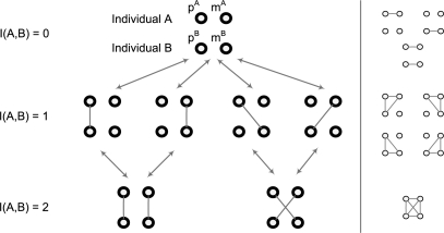
Denote I(a, b) the number of IBD sharing between two alleles a and b, i.e. I(a, b) = 1 if they are IBD and I(a, b) = 0 otherwise. Between two individuals A and B, the number of IBD sharing is defined as I(A, B) = max(I(p^A, p^B)+I(m^A, m^B), I(p^A, m^B)+I(m^A, p^B)). The four alleles of two individuals have a total of 15 different combinations of IBD sharing status as shown in Figure 3. When ignoring the IBD sharing between paternal and maternal alleles of an individual and there are seven distinct combinations (Fig. 3, left). For simplicity, we only consider these seven states in this study and they are the hidden states of the HMM for a pair of individuals. Notice that it is possible to derive a HMM using all 15 states, but the derivation of transition probabilities gets more involved. For human pedigrees, this approximation will not cause many problems because in general human pedigree structures are not too complex.

Fig. 3.

IBD sharing states between two individuals. Righthand side are the states not considered in this study.

Denote the state vector s = (I₁, I₂, I₃, I₄), where I₁ = I(p^A, p^B), I₂ = I(p^A, m^B), I₃ = I(m^A, p^B), I₄ = I(m^A, m^B). Each state is uniquely represented by one state vector. Given a small inter-marker distance, it is rare opportunity for more than one recombination to occur, so we only allow transitions between states themselves and transitions between neighboring states, i.e. states that differ at most one allele IBD sharing status, ‖s−s′‖≤1. Therefore, Figure 3 (left) actually represents our HMM structure for a pair of individuals, with one additional transition from each state to itself omitted. Conditional on the pair being in state s at locus i, the probability that they are in state s′ at locus i+1, denoted as f(s′|s), is essentially the product of two independent HMM chains described in section 2.2. That is, f(s′|s) = P(I′_j|I_j)P(I′_k|I_k), where 1≤j, k≤4 are two independent coordinates in the 4D vectors of s and s′, which means the two alleles in I_k are different from the two alleles in I_j, and the two alleles in I_k (I_j) are the same as those in I′_k (I′_j). P(I′_j|I_j) and P(I′_k|I_k) are the transition probabilities described in Figure 2. The transition probabilities of our model (Fig. 3, left)

for all ‖s−s′‖ ≤ 1, are proportional to the conditional probabilities f(s′|s). It is worthy of mention that though we ignore inbreeding, our method can still be applied to looped pedigrees because the IBD between paternal and maternal alleles does not affect the IBD sharing number between two individuals. However, for looped pedigrees, P(I′_j|I_j) and P(I′_k|I_k) might not be independent and such derived probability P(s′|s) is an approximation of the actual probability. We will show later in the experiments that our method works well for both inbreeding and non-inbreeding families. We are currently exploring the extension of the algorithm to all 15 identity states.

Denote G(a, b) the number of IBS between two alleles a and b, i.e. G(a, b) = 1 if they are IBS and G(a, b) = 0 otherwise. The number of IBS between two individuals A, B: G(A, B) = max(G(p^A, p^B)+G(m^A, m^B), G(p^A, m^B)+G(m^A, p^B)), i.e. the number of the same type of alleles between these two genotypes. To derive the emission probabilities, we separate the seven states into three classes according to their number of IBD, because the emission probabilities of G(A, B) only depend on I(A, B) and different states with the same I(A, B) will have the same emission probabilities. Similarly to the derivation of emission probabilities of the basic model in section 2.2, the probability distribution of the IBS number G(A, B) between two individuals given their IBD sharing number I(A, B) can be specified directly based on their definitions, which is shown in Table 1. In practice, one also needs to take into account the effect of missing genotypes and genotyping errors. We leave the details about emission probabilities after considering missing/errors in Supplementary Material.

Table 1.

Emission probability of an IBS number (G) given an IBD number (I), where p and q = 1−p are population allele frequencies

G	I	P(G|I)
0	0	2p2q2
1	0	4p3q+4pq3
2	0	p4+q4+4p2q2
0	1	0
1	1	2pq
2	1	p2+q2
0	2	0
1	2	0
2	2	1

Given the transition probabilities, the emission probabilities and the IBS numbers between two individuals from their observed genotypes, we can use the Viterbi algorithm to decode the most likely IBD sharing status between any pair of individuals within a pedigree. For each pair of individuals, standard dynamic programming for Viterbi is O(mK²), where m is the number of SNPs and K is the number of states (a constant). There are a total of O(n²) pairs of individuals for a family of n individuals, so the overall time complexity is O(n²m).

2.5 Incorporating background IBD sharing

Since the human being is a relatively young species, even between two seemingly unrelated individuals, one can still observe long segments of IBS regions. From one perspective, this can be attributed to the LD between SNPs. From another perspective, this is essentially due to the unobserved relatedness in history among humans. This type of background sharing coupled with IBD sharing within a pedigree will lead to biased inference of true IBD status. However, it is impossible to explicitly model this type of relatedness because the relationship of individuals beyond the pedigree is generally unknown and they may have been separated by many meioses and may have multiple common ancestors. Recently, Purcell et al. (2007) proposed a model to approximate the relativeness for ‘unrelated’ individuals, which also use an HMM. To address this problem for members within a pedigree, we extend our model by adding a background IBD (Bg-IBD) state to fit the hidden relatedness between two individuals beyond the relatedness that is observed through the available pedigree structure.

We first extend the basic two-state allelic HMM in Figure 2 to a three-state allelic model by adding the Bg-IBD state (Fig. 4). The transition probability from IBD state to itself stays the same. Both the states Bg-IBD and the state Non-IBD imply that the two alleles are not IBD within the pedigree. Therefore, the transition probabilities from these two states to the state IBD is the same. From the perspective of the state IBD, transitions to states Bg-IBD and Non-IBD imply that recombination events break the inheritance path between the two alleles. We assume that the transition probabilities to Bg-IBD and Non-IBD are just proportional to the probabilities of observing Bg-IBD and Non-IBD. By applying these restrictions and also utilizing the relationship between marginal and transition probabilities, we have

If we take P(Bg-IBD) and P(Bg-IBD_i+1|Bg-IBD_i) as parameters to fit the background effect, the above transition probabilities as well as P(Non-IBD_i+1|Bg-IBD_i), P(Bg-IBD_i+1|Non-IBD_i) and P(Non-IBD_i+1|Non-IBD_i) can be calculated based on them. Intuitively, P(Bg-IBD) represents the kinship between the two individuals beyond the pedigree and P(Bg-IBD_i+1|Bg-IBD_i) represents the number of meioses they are apart on each of the possible inheritance paths connecting them. In our experiments, we vary the number of meioses k and use (1−ϖ)^k to approximate P(Bg-IBD_i+1|Bg-IBD_i), where ϖ is the recombination fraction and can be calculated using Haldane's mapping function based on the marker interval genetic distance. P(Bg-IBD) will be estimated directly from the model.

Fig. 4.

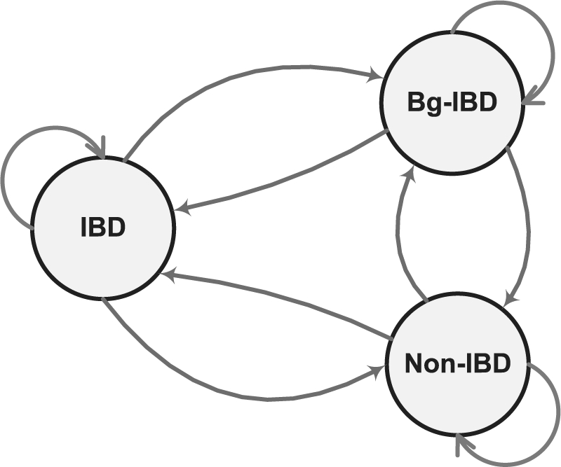
The three-state transition model of the IBD status between two alleles a and b.

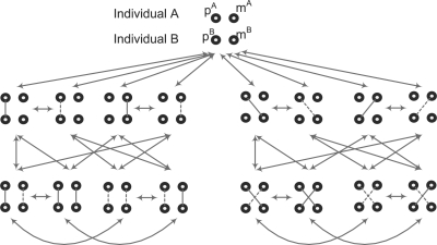
To incorporate Bg-IBD sharing into the HMM between a pair of individuals, we modify the model structure in Figure 3 by adding one more state for each original state labeled as I(A, B) = 1 and adding three more states for each original state labeled as I(A, B) = 2. Following the argument in Section 2.4, transition probabilities for such a model can be derived from the above allelic HMM in Figure 4. The complete transition model is shown in Figure 5.

Fig. 5.

The complete transition model of IBD sharing states between two individuals. Solid lines indicate actual IBD and dashed lines indicate Bg-IBD.

2.6 Constructing pedigree-wise IBD sharing

By decoding the seven-state HMM shown in Figure 3, we can obtain not only the IBD number between two individuals, but also the IBD relationship between four alleles. However, one should notice that the inferred IBD state between alleles could be arbitrary, even when the inferred IBD number is correct. This is because the states of IBD sharing number 1 are symmetric and may not be distinguishable (e.g. for a pair of siblings, the paternal and maternal assignments are interchangeable). Therefore, in order to build the global IBD sharing map from all pairwise IBD relationships, we need a post-processing step. In our current implementation, for each locus, we simply enumerate all possible ways of allele grouping and check its consistency with all pairwise relationships. If there are no consistent grouping, which means errors have occurred when decoding some pairwise IBDs, we simply drop this SNP. If there are more than one consistent groupings, we randomly select one. We notice that there are rooms for further improvement and we will investigate more efficient combination approaches in the future.

3 EXPERIMENTAL RESULTS

We test the proposed method using two real datasets and one simulated dataset. The first real dataset consists of 112 nuclear families each with two parents and two children. We assume that the genotypes of both parents are not available and infer the IBD status for each pair of siblings. We then compare the results of IBD changing breakpoints with the recombination breakpoints inferred by our previous algorithm Mendelian constrained maximum likelihood (MML) (Li et al., 2010) using genotypes of both parents and children. The second dataset is a pedigree of size 15, among which only seven members are typed. We infer IBD sharing between all pairwise relatives (other than parent–child pairs) and generate a pedigree-wise IBD sharing map. To evaluate the correctness of our approach on big pedigrees, we generate simulated datasets using the same pedigree structure and missing pattern.

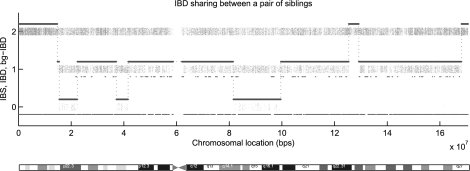
For the sib-pair data, we have 32 250 SNP markers on chromosome 6 genotyped using Illumina 500K chips. The total region contains 170 million base pairs with the average marker interval distance about 5 kb. Missing genotype rate is 0.12% and typing error rate (as reflected by Mendelian inconsistency) is 0.11%. Figure 6 shows the IBS status, the inferred IBD status and Bg-IBD status between a randomly selected pair of siblings. The dotted bar indicates the density of markers of IBS number 0, 1 and 2, at that chromosomal location. The bold blue line and the thin red line indicate the inferred IBD number and Bg-IBD number, respectively. Along the chromosome, the Bg-IBD number changes much more frequently than the pedigree IBD number. This result is consistent with the fact that Bg-IBD is generated by long inheritance paths with many meioses. Therefore, the shared segments are much smaller compared with lengths of the IBD segments within a pedigree. We notice that the centromere region around 60 Mb has no markers, which forms a gap of 3 million base pairs. This will cause our method to create some unexpected IBD status jumps. We ignore any IBD status change around the centromere region.

Fig. 6.

IBD sharing between two siblings. The dotted bar indicates the density of markers of IBS number 0, 1 and 2. The bold line is the pedigree IBD sharing number and the thin line is the Bg-IBD sharing number.

To systematically evaluate the correctness of inferred IBD sharing regions of all sibling pairs, we compare our result with that inferred by our previous algorithm MML (Li et al., 2010), which is a Mendelian law-based method and use genotypes of both parents and children. MML infers the inheritance pattern by using Mendelian constraints between parents and children. It achieves high accuracy on dense SNP data, when all members of a pedigree are genotyped. From 112 families with two siblings, MML infers 322 paternal and 535 maternal recombination events. For the proposed method, recombination positions can be obtained from the IBD status change points. By setting the Bg-IBD level to be 200 meioses apart, the new approach infers 812 recombination breakpoints, among which 776 are consistent with the results of MML. The remaining 36 breakpoints are due to background effect but are falsely classified as IBD sharing within pedigrees. The approach misses 81 out of all 857 breakpoints. These breakpoints are caused by changes in the inheritance pattern in the pedigrees but are falsely classified as Bg-IBD sharing. By setting the Bg-IBD level to be more meioses apart, we can increase the sensitivity of the method in detecting recombination. However, doing so will reduce the specificity, and vice versa. Table 2 presents the false positive rates and false negative rates by setting the Bg-IBD level to be 100, 200, 300, 400 meioses apart.

Table 2.

Error rates under different Bg-IBD levels (100–400 meioses)

No. of meioses	100	200	300	400
False positive	23/768	36/812	83/875	111/912
	0.030	0.044	0.095	0.122
False negative	112/857	81/857	65/857	56/857
	0.131	0.095	0.076	0.065

A total of 857 recombinations are detected by the Mendelian law and are used as the reference. False positives are recombinations reported by our method but not in the reference. False negatives are the recombinations in the reference but missed by our method.

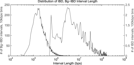
To further analyze this phenomenon, we examine the difference of the lengths of IBD sharing intervals between those inferred as actual IBD and those inferred as background sharing. If we set the Bg-IBD level to be 200 meioses apart, the length distribution of intervals is shown in Figure 7. The average length of IBD regions is 37.5 Mb (SD 4.1 Mb), while the average length of Bg-IBD regions is 362 kb (SD 357 kb). Though these two distributions are quite distinguishable, they still have overlapped tails. Some short segments of pedigree IBD sharing will be inferred as background sharing and some long segments of Bg-IBD sharing will be inferred as real IBD sharing. If we increase the number of meioses for the background effect, we will shift its distribution leftward to be more distinct from the pedigree effect. This will increase the sensitivity while reduce the specificity of the method. The situation is reversed, if we reduce the number of meioses to shift the background effect distribution rightward to be more mixed with the pedigree effect. We are currently researching the problem how to automatically fit the Bg-IBD.

Fig. 7.

Length distributions of IBD and Bg-IBD intervals. The chart puts both distributions together with x-axis on a logarithmic scale. The left-hand curve is from Bg-IBD intervals and the right-hand curve is from IBD intervals.

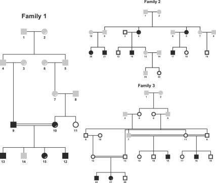
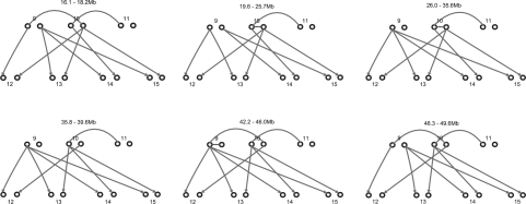
We further apply the approach on a family with 15 members (Fig. 8, Family 1), among which only 7 members are genotyped using Affymetrix array 6.0 (∼1 million SNPs). We investigate a region of 35 Mb on chromosome 22 with 11 554 markers. The missing rate is 2.74% and the typing error rate (as reflected by Mendelian inconsistency) is 2%. Figure 9 shows the IBD sharing between two members (9 and 10) of the family with segments of IBD sharing at each end of the chromosome. By analyzing the IBD sharing between all pairs of the seven genotyped individuals in this family, we can reconstruct the global IBD sharing graph as shown in Figure 10, where alleles linked by lines are IBD. In this example, the IBD alleles between individuals 9, 10 and 11 are linked together without enumerating the transmissions from their ancestors. We can observe the changes of inheritance patterns from one chromosomal region to another, which can be used for non-parametric linkage analysis. In this example, the first region (16.1–18.2 M) is consistent with the dominant model of the disease.

Fig. 8.

Families 1, 2 and 3. Gray-colored individuals are not genotyped. Black-colored individuals are diseased and white-colored individuals are normal.

Fig. 9.

IBD sharing between members 9 and 10 of Family 1. The layout of the figure is the same as the layout of Figure 6.

Fig. 10.

Global IBD sharing graphs for different chromosomal regions. Alleles connected by an arc or arrow are IBD.

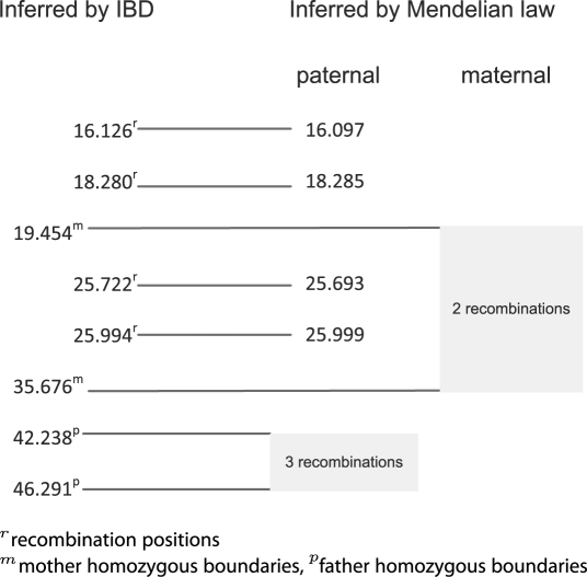
The global IBD map suggests that there is an IBD sharing between the paternal and the maternal alleles of member 9 extending from 42 to 46 Mb, an IBD sharing between the paternal and maternal alleles of member 10 extending from 19 to 35 Mb (dashed red line in Fig. 11). This is indeed the case because both regions have consecutive homozygous genotypes. We further analyze the nuclear family formed by members 9 and 10 and their children using MML and compare recombination breakpoint positions inferred by the two approaches (Fig. 11). In this case, both algorithms identify nine recombination events. Among them, both approaches accurately identify four breakpoints with high precision. All the other five breakpoints are in the two extended homozygous regions of members 9 and 10, neither methods can localize the recombination positions precisely because of the ambiguity. We can still infer the number of recombination events occurring in such a region by comparing the transmission patterns before and after the region. We annotate the homozygous regions of both parents as shaded areas in Figure 11 and indicate the inferred number of recombinations in each region.

Fig. 11.

Comparison of recombination positions inferred by the proposed method and by the Mendelian law. Numbers are shown in the unit of megabase pair. Shaded areas are the regions where the parents are homozygous.

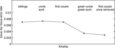
To evaluate the reliability of the inferred IBD relationship for different types of relationships, we further generate a simulated dataset to mimic the same pedigree (Fig. 8, Family 1) using the same genotype missing rate, typing error rate and the same marker map on chromosome 22. We randomly assign haplotypes to founders of the pedigree and assume random transmission of these haplotypes to descendants with possible recombinations at each meiosis. Recombination is modeled at a rate of 1cM/Mb assuming a Poisson distribution. The haplotypes used in the founders are generated from other families in the same study using the haplotype inference method MML (Li et al., 2010). We run the simulation 1000 times and compare the inferred IBD sharing regions with the actual IBD sharing regions for each pair of individuals. Results of some representative pairs, including 10 and 11 (siblings of untyped parents), 12 and 13 (siblings of typed parents), 11 and 12 (aunt and nephew) and 9 and 10 (distant relatives) are presented in Table3, with the inheritance path between all pairs of alleles in each pair of individuals in the last row, which gives the degree of relatedness of each pair of individuals. We collect the breakpoints between IBD and Non-IBD regions and compare the inferred regions with the actual ones. For different types of pairs, the approach has similar false positive and false negative rates. Though for more distant related pairs, false negative rate gets slightly higher. This is due to the fact that for distant-related pairs, their pedigree IBD sharing is more likely to be mixed with the background sharing. The precision value shows the average distance from an inferred breakpoint to the actual breakpoint. It exhibits the same trend that the inferred IBD boundaries are more ambiguous if two individuals are more distant related. In general, the proposed method detects ∼85% of the breakpoints between IBD and Non-IBD regions. About 5% of the reported breakpoints are false positives, mainly caused by Bg-IBD sharing and/or genotyping errors. Supplementary Figure S1 shows some typical errors in inferred IBD regions. We also run simulations on two big pedigrees of 23 and 22 members (Families 2 and 3, Fig. 8). All these families are from the same study as Family 1. Figure 12 shows the locus-by-locus IBD inference accuracy. The average error rate is <1% for all related pairs of different kinships, which is much lower than the error rates of breakpoints. This is due to the fact that the misclassified IBD segments are short ones near the overlapping tails of IBD and Bg-IBD (Fig. 7) such that they do not contribute much to the overall locus-by-locus discrepancies. The locus-by-locus error rate is lower for distant-related individuals and again this is because distant relatives have shorter shared IBD segments.

Table 3.

Accuracy in identifying IBD breakpoints for different pairs of individuals of Family 1

Family 1	10–11	12–13	11–12	9–10
False positive	0.068	0.043	0.046	0.042
False negative	0.124	0.123	0.134	0.160
Precision	187kb	193kb	238kb	287kb
Inheritance path	4h2	4h2+8h7	4h3+4h6	4h5

IBD breakpoints are chromosomal locations where the IBD sharing number between two individuals changes. The precision value shows the average distance between an actual breakpoint and the inferred one.

Fig. 12.

Locus-by-locus IBD inference error for different relatives in Families 1, 2 and 3.

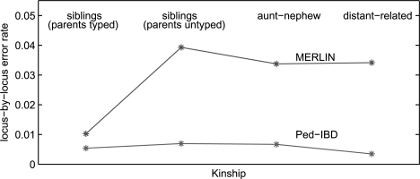
We compare the IBD inference accuracy of our program (Ped-IBD) with MERLIN (Abecasis et al., 2002). Both Ped-IBD and MERLIN can be configured to output the posterior probabilities of IBD 0, 1 and 2 at each locus, and we take the IBD number of the highest probability as their inferences. For dense SNP markers, the highest probability is usually close to 1, so the inference is quite deterministic. Figure 13 shows the locus-by-locus error rates for pairs of individuals of different kinships in Families 1. Ped-IBD has better accuracy than MERLIN for all types of related pairs especially on siblings with untyped parents and distant-related individuals. Table 4 presents the running time of Ped-IBD and MERLIN on Family 1, 2 and 3 and on different marker numbers. Ped-IBD is implemented in Matlab and we use the precompiled Linux version of MERLIN. We run both programs on a Dell PowerEdge 2900 Server with Xeon E5430 Dual Processor and 32G memory. Ped-IBD shows a time complexity pattern linear to marker numbers and quadratic to the number of typed individuals. MERLIN slows down significantly on big families and consume exponentially more memory. We are not able to obtain results from MERLIN in certain categories due to insufficient memory. These results show the advantage of our approach in both accuracy and efficiency over traditional linkage analysis methods.

Fig. 13.

Comparison of IBD inference accuracy of Ped-IBD and MERLIN for persons of different kinships in Family 1.

Table 4.

Running time (in seconds) for different marker numbers (10−10k) and pedigree structures (Families 1, 2, 3), compared with MERLIN

No. of markers	Ped-IBD			MERLIN
	1	2	3	1	2	3
10	0.17	0.41	0.84	0.08	6.14	89
20	0.20	0.70	1.40	0.19	16.86	63
50	0.55	1.34	2.43	0.39	39.98	251
100	0.93	2.54	4.67	0.89	76.70	–
10k	91	252	456	95	–	–

The sizes of these families are 15(7), 23(11) and 22(17), the numbers in the parenthesis are typed individuals.

4 DISCUSSION

Traditional linkage analysis models the transition of inheritance vectors from one locus to another as a complex multiple-state Markov chain and derive the probability of IBD sharing. Given the current density of SNP markers, the inheritance pattern of a pedigree can usually be fixed by applying the Mendelian law of inheritance, which basically means that one can almost ‘observe’ IBD sharing states. However, the use of Mendelian law requires that all or most members of a family should be genotyped, which is not practical for studies involving large pedigrees. To avoid enumerating the genotypes of the untyped members, we extract the inheritance information between two individuals by tracing all possible inheritance paths between them. By doing so, we can directly model the IBD sharing status between any pair of individuals without considering the actual transmission across their ancestors. From the pairwise IBD relationship, we can build the global IBD sharing map of the whole pedigree for genotyped members. We use our method to infer the recombination positions in nuclear families with two siblings. Our method detects >90% of the recombination positions and has <5% false positive reports. Experiments on large pedigrees show that the method is accurate in identifying IBD and Non-IBD boundaries in both closely and distantly related individuals. We further incorporate the Bg-IBD state into our HMM model to deal with background LD between markers. By adjusting the background IBD level, we can tune the sensitivity and specificity of the method accordingly. Regardless, long segments of pedigree IBD sharing are always safely recovered in most cases. We also compare our algorithm with MERLIN and it shows that our method has both better accuracy and efficiency. By partitioning the chromosome into regions of different inheritance patterns, we can generate statistics for assessing the linkage of a chromosomal region with the disease. Based on the inferred IBD, we will further incorporate linkage analysis into our model.

REFERENCES

- Abecasis GR, Wigginton JE. Handling marker-marker linkage disequilibrium: pedigree analysis with clustered markers. Am. J. Hum. Genet. 2005;77:754–767. doi: 10.1086/497345. [DOI] [PMC free article] [PubMed] [Google Scholar]
- Abecasis GR, et al. Merlin–rapid analysis of dense genetic maps using sparse gene flow trees. Nat. Genet. 2002;30:97–101. doi: 10.1038/ng786. [DOI] [PubMed] [Google Scholar]
- Elston RC, Stewart J. A general model for the genetic analysis of pedigree data. Hum. Hered. 1971;21:523–542. doi: 10.1159/000152448. [DOI] [PubMed] [Google Scholar]
- Geiger D, et al. Speeding up HMM algorithms for genetic linkage analysis via chain reductions of the state space. Bioinformatics. 2009;25:i196–i203. doi: 10.1093/bioinformatics/btp224. [DOI] [PMC free article] [PubMed] [Google Scholar]
- Gudbjartsson DF, et al. Allegro version 2. Nat. Genet. 2005;37:1015–1016. doi: 10.1038/ng1005-1015. [DOI] [PubMed] [Google Scholar]
- Karigl G. A recursive algorithm for the calculation of identity coefficients. Ann. Hum. Genet. 1981;45(Pt 3):299–305. doi: 10.1111/j.1469-1809.1981.tb00341.x. [DOI] [PubMed] [Google Scholar]
- Keith JM, et al. Calculation of ibd probabilities with dense snp or sequence data. Genet. Epidemiol. 2008;32:513–519. doi: 10.1002/gepi.20324. [DOI] [PubMed] [Google Scholar]
- Kruglyak L, et al. Parametric and nonparametric linkage analysis: a unified multipoint approach. Am. J. Hum. Genet. 1996;58:1347–1363. [PMC free article] [PubMed] [Google Scholar]
- Lander ES, Green P. Construction of multilocus genetic linkage maps in humans. Proc. Natl Acad. Sci. USA. 1987;84:2363–2367. doi: 10.1073/pnas.84.8.2363. [DOI] [PMC free article] [PubMed] [Google Scholar]
- Li X, Li J. An almost linear time algorithm for a general haplotype solution on tree pedigrees with no recombination and its extensions. J. Bioinform. Comput. Biol. 2009;7:521–545. doi: 10.1142/s0219720009004217. [DOI] [PMC free article] [PubMed] [Google Scholar]
- Li X, et al. Detecting genome-wide haplotype polymorphism by combined use of mendelian constraints and local population structure. Pac. Symp. Biocomput. 2010;15:348–358. doi: 10.1142/9789814295291_0037. [DOI] [PMC free article] [PubMed] [Google Scholar]
- Purcell S, et al. Plink: a tool set for whole-genome association and population-based linkage analyses. Am. J. Hum. Genet. 2007;81:559–575. doi: 10.1086/519795. [DOI] [PMC free article] [PubMed] [Google Scholar]
- Sobel E, Lange K. Descent graphs in pedigree analysis: applications to haplotyping, location scores, and marker-sharing statistics. Am. J. Hum. Genet. 1996;58:1323–1337. [PMC free article] [PubMed] [Google Scholar]
- Thompson EA. The Johns Hopkins Series in Contemporary Medicine and Public Health. Baltimore; 1986. Pedigree Analysis in Human Genetics. [Google Scholar]
- Wright S. Coefficients of inbreeding and relationship. Am. Nat. 1922;56:330–338. [Google Scholar]
Associated Data
This section collects any data citations, data availability statements, or supplementary materials included in this article.