Estimating Uncertainty in Brain Region Delineations

Abstract

This paper presents a method for estimating uncertainty in MRI-based brain region delineations provided by fully-automated segmentation methods. In large data sets, the uncertainty estimates could be used to detect fully-automated method failures, identify low-quality imaging data, or endow downstream statistical analyses with per-subject uncertainty in derived morphometric measures. Region segmentation is formulated in a statistical inference framework; the probability that a given region-delineating surface accounts for observed image data is quantified by a distribution that takes into account a prior model of plausible region shape and a model of how the region appears in images. Region segmentation consists of finding the maximum a posteriori (MAP) parameters of the delineating surface under this distribution, and segmentation uncertainty is quantified in terms of how sharply peaked the distribution is in the vicinity of the maximum. Uncertainty measures are estimated through Markov Chain Monte Carlo (MCMC) sampling of the distribution in the vicinity of the MAP estimate. Experiments on real and synthetic data show that the uncertainty measures automatically detect when the delineating surface of the entire brain is unclear due to poor image quality or artifact; the experiments cover multiple appearance models to demonstrate the generality of the method. The approach is also general enough to accommodate a wide range of shape models and brain regions.

1 Uncertainty in Brain Region Delineations

1.1 Importance of Uncertainty Estimation in Brain Region Delineations

Structural magnetic resonance imaging (MRI) is a technology for measuring biological properties of the brain. A widespread methodology for large-scale epidemiological studies is to collect MRI scans of a cohort of subjects, delineate brain regions on those scans using manual or automated methods, and relate morphometric measures derived from those region delineations to clinical variables of interest. Studies of this sort have played an important role in clarifying the biological course of a range of neurological disorders, including multiple sclerosis and dementia [9] [7].

This paper provides a method for quantifying uncertainty in brain region delineations. Once the uncertainty in a brain region delineation is known, we can use this information to identify and possibly discard images whose region delineations have high uncertainty and therefore may have been segmented imprecisely. Our formulation of uncertainty is chiefly concerned with the precision, rather than the accuracy, of the delineating boundaries of brain regions. As with every measurement, both the accuracy and precision of the delineating surface determine the validity of inference made from their derived measures: accuracy is the degree to which the measurement is close to the true value of the quantity being measured, while precision is the degree to which repeated measurements provide similar values [8]. If a measurement is imprecise, we cannot be certain whether the measurement value arises from underlying biological phenomena or random fluctuations in the measurement process. Our approach is to use a statistical sampling procedure to simulate the repeated measurement of the same brain region boundary by an automated segmentation method, and assess whether the segmentation method tells us that a diverse, widely-scattered set of boundary surfaces delineate the region equally well.

The uncertainty in a brain region delineations obtained via automated methods can be affected by several factors. Poor image quality or low contrast between two brain regions can both lead to images that are hard to segment precisely. Further, measurement uncertainties are exacerbated when the models of brain appearance and shape used by an automated method are oversimplified or invalid. In these cases, a measurement can be imprecise; to our knowledge, there are currently no automated tools for quantifying measurement precision so these errors may be left undetected in the absence of time-consuming, tedious manual checking of segmentation results.

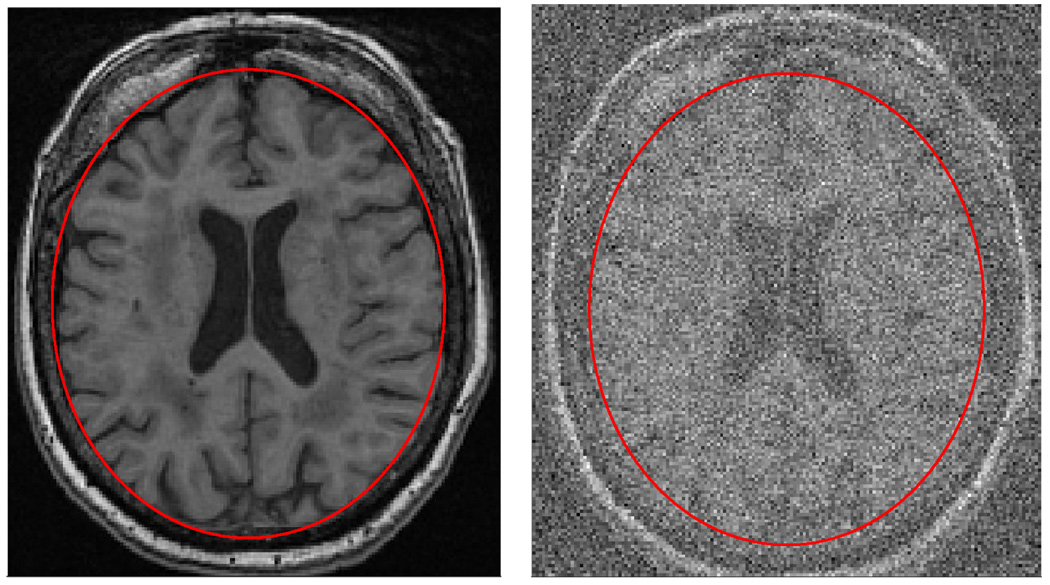
For example, imagine that the area of the ellipses in figure 1 are to be used to estimate the volume of the brain in the image. When making this derived measurement for the blurred image in figure 1, we could not be sure what size the ellipse should be in order to best approximate the brain contour since the image is blurry and the boundary between the skull and the brain is uncertain. This is an important concern because the size of the ellipse will determine the computed volume, which in turn will be used in a statistical analysis to test a hypothesis about relationships between brain volume and other clinical measures. Thus, uncertainty in derived measures give rise to errors in the data which in turn result in errors in the statistical analyses.

Fig. 1.

The image on the right is the result of applying heavy white noise to the same image shown on the left. The ellipse on the left image is a region-delineation that partitions the image into brain region(inside the ellipse) and the non-brain region(outside of the ellipse). The ellipse on the right is the same as that on the left but due to the noise, it is no longer clear that the ellipse on the right truly does partitions the image correctly. Given the noisy image, different ellipses with different areas seem to fit the brain equally well.

Most current fully automated segmentation methods cannot detect corrupted images or grossly incorrect delineations. Our hypothesis is that this is partly due to the fact that modern segmentation methods suffer from the inability to incorporate a quantitative estimate for the precision of reported measurements and that there is currently not a standard method for obtaining such estimates. Though the uncertainty in this example was synthetically produced, there are many real sources of uncertainty in image delineation. For example, blurry or ”‘ghosted”’ images can lead to measurement uncertainty as well as images of brains with large pathologies which can sometimes deviate from the model assumptions of the segmentation method being used for the study.

1.2 Overview of Our Approach

A convenient way of formulating region-based delineation that encompasses many popular methods involves a Bayesian framework. The Bayesian approach seeks an answer to the question, ’what is the most probable delineating contour or surface of a desired region given the current image?’ If we let I represent the image to be segmented and θ be a vector of parameters used to represent the shape of the delineating surface, then we can mathematically phrase this question by asking for a solution to the following conditional probability equation:

$$\widehat{\theta }=\text{arg}\underset{\theta }{\text{max}}P(\theta |I)$$ (1)

P(θ|I) is the posterior probability of the parameters θ given the image, I. By Bayes Theorem equation 1 can be written as

$$\widehat{\theta }=\text{arg}\underset{\theta }{\text{max}}L(I|\theta )q(\theta ).$$ (2)

L(I|θ) is the image model: it is the likelihood of obtaining the image I given that the shape parameters are θ. The q(θ) term is known as the shape model; it is the prior probability that the region will take on the shape described by θ, regardless of the image I.

We estimate uncertainty in region delineation by using Markov Chain Monte Carlo (MCMC) to sample a series of θ from P(θ|I) and using the samples to approximate the solution to expectation integrals that give measures of uncertainty in the position of θ̂. Because morphometric measures such as volume and surface area are often derived from θ̂ and related to clinical variables in statistical analyses, the uncertainty measures can provide measures of uncertainty in the derived measures. We will demonstrate that the method is modular in the sense that it can be used in combination with a broad range of currently existing region delineation methods to estimate an optimal region-delineating surface and uncertainty in the surface.

1.3 Related Work

To our knowledge, the automated estimation of uncertainty in a single region delineation has not been addressed directly in the neuroimaging literature. The closest work to ours may be Simultaneous Truth and Performance Level Estimation (STAPLE) [12]. STAPLE formulates the region delineation problem in a probabilistic setting similar to ours, but is focused on using a statistical inference method to estimate variability across multiple manual delineations of the same region, along with the underlying ground-truth boundary surface. Here, in contrast, we are concerned with using statistical methods to estimate, for each input image and region, the delineating surface uncertainty that is inherent to a particular automated segmentation method. Uncertainty estimation differs from, and is more general than, segmentation validation method. Not only can uncertainty estimates be used to assess the quality of an image and/or segmentation, but it can also be used to enhance the statistical analysis that the segmentation was computed for in the first place. Outside of neuroimaging, estimating uncertainty in model parameters has been addressed in many fields. For example, [6] and [2] both use MCMC methods similar to the one presented here for estimating uncertainty in water catchment models and extra solar orbits respectively. Sampling methods such as MCMC have been used to represent uncertainty in time-varying variables being tracked by systems in computer vision and mobile robotics [3] [4]; and finally, some authors have used MCMC and related sampling methods as a means of finding extrema of complex probability distributions in computer vision problems, rather than for uncertainty estimation per se [1] [11].

2 Metropolis-Hastings and Markov Chain Monte Carlo

Monte Carlo integration is a numerical integration scheme used to estimate the expectation of a function f(θ) under a given distribution such as P(θ|I). Monte Carlo integration works by drawing sample θ values from P(θ|I). For example, let {θ₀, θ₁, …, θ_n} be a sequence of independent identically distributed (i.i.d) random variables sampled from P(θ|I). Then the law of large numbers tells us that:

$$\frac{1}{n}{\displaystyle \sum _{t=1}^{n}f({\theta }_t)\to E_{P(\theta |I)}[f]={\displaystyle {\int }_{-\mathrm{\infty }}^{\mathrm{\infty }}f(\theta )P(\theta |I)d\theta }}$$ (3)

Thus, by evaluating the integrand at a sequence of points drawn from P(θ|I), Monte Carlo integration can approximate the population expectation for f under P(θ|I) to an arbitrary degree of precision by a sample mean computed from a sufficiently large sample.

The major assumption in Monte Carlo integration is that there exists a way to generate independent samples from an arbitrary distribution. This is not a trivial assumption because in many cases, P(θ|I) is highly non-standard and therefore difficult to sample from directly. The theory of Markov Chains and specifically the Metropolis-Hastings Algorithm helps to overcome this difficulty.

MCMC refers to a group of algorithms used to estimate E_{P (θ|I)} [ f ] by computing the mean of f over a set of samples drawn from a Markov chain whose stationary distribution is P(θ|I). The Metropolis-Hastings Algorithm is the most widely-used MCMC variant. Metropolis-Hastings simulates a Markov chain that transitions from a current state, θ_n, to a subsequent state θ_n+1 based on a stochastically chosen candidate state, γ. γ is generated by sampling from a proposal distribution, Q(γ|θ_n) over the space of all possible states. γ is either accepted− θ_n+1 = γ − or rejected− θ_n+1 = θ_n depending on whether or not the following function passes a threshold:

$$\alpha ({\theta }_{n,}\gamma )=\mathit{\text{min}}(1,\frac{P(\gamma |I)Q({\theta }_n|\gamma )}{P({\theta }_n|I)Q(\gamma |{\theta }_n)})$$ (4)

Hastings (1970) showed that the sequence of random variables that generated by this algorithm is a Markov chain whose states are eventually drawn from the distribution P(θ|I) after an appropriate number of initial states known as the burn-in period.

In practice, the three major design choices in MCMC are the selection of the proposal distribution, the criterion for determining that the burn-in period has ended, and the criterion for determining how many states to sample from the Markov chain after the burn-in period to estimate the required expectation. Once these design choices have been addressed, equation 3 tells us we can approximate E_{P (θ|I)}[ f ] in a Markov chain with an m-state burn-in period and n states required for expectation estimation as follows:

$$E_{P(\theta |I)}[f]\approx \frac{1}{(n-m)}{\displaystyle \sum _{j=m+1}^{m+1+n}f({\theta }_j).}$$ (5)

3 Estimating Measurement Uncertainty with MCMC

3.1 The MCMC Approach

Given that a region-based delineation method as formulated in equation 2 provides an estimate θ̂ of the region delineating surface, we set θ̂ to be the initial state for a Markov chain, i.e. θ₀ = θ̂, and use Metropolis-Hastings MCMC to construct the rest of the Markov chain. We approximate the expectations of two different functions. First we estimate E[g(θ)] = E[||θ̂ −θ||²]. This expectation is equal to the variance of P(θ|I) in the event that θ̂ is the mean of.

We also compute the expectation of the following characteristic function:

$${\chi }_{\rho }\left(\theta \right)=\{\begin{array}{c}1\text{if}\frac{|P(\widehat{\theta }|I)-P(\theta |I)|}{P(\widehat{\theta }|I)}\le \rho \hfill \\ 0\text{otherwise}.\hfill \end{array}$$

Geometrically, E[χ_ρ(θ)] is the volume of the shape parameter space whose posterior probability is within a relative difference of ρ to the optimal delineating surface. Intuitively, this provides a sense of the uniqueness of θ̂. That is, if E[χ_ρ(θ)] is large when ρ is small, then there are many diverse delineating surfaces that fit the image data just as well as the optimal surface; that is, there are many θ whose P(θ|I) is nearly equal to P(θ̂|I). ¹ We used a multivariate normal distribution, centered about the current state θ_n, as our proposal distribution.

4 Experiments

4.1 Overview

To demonstrate that this approach is modular with respect to image models, we test the method on two different methods for delineating the entire brain (a.k.a. ”skull stripping”). Both use an ellipse shape model in which the size and rotation of the ellipse is fixed, and the two free parameters represent the x and y coordinates of the ellipse center. The first image model is the MeanSquaresPointSetToImageMetric (or MSPSM) model from the Insight Toolkit (ITK) software package. The MSPSM image model computes the average mean square difference between the pre-defined pixel values of a provided point set and intensity values of an image.

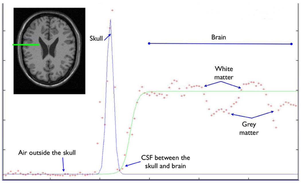
The second image model makes use of Intensity Profiles(IP, see Figure 2). It first computes the outward pointing unit normal vector to the surface at each point on the delineating surface. An array is constructed whose components are the image intensities of uniformly sampled points along the normal; a gaussian curve (whose peak represents the skull) and a logistic curve (whose low and high levels represent cerebrospinal fluid and parenchyma respectively) are fit to the array of intensities through maximum likelihood estimation. A new position of the brain-delineating surface along the surface normal is proposed based on the low points of the gaussian and logistic curves; the contribution of the surface point to the likelihood term is inversely proportional to the distance between the current position of the brain-delineating surface and the proposed one. Similar image models are used in [5] and [10].

Fig. 2.

An intensity profile going across the brain-skull interface has the general form of a Gaussian and logistic curve superimposed. From left to right, intensities along the profile correspond to air, skull, CSF, and parenchyma respectively

4.2 Data

The protocol for testing the MCMC uncertainty estimation method is as follows. First, the skull stripping of a 2D axial slice from a 3D T1 weighted MRI image is computed. Next, the output from the skull stripping, along with the 2D slice are given as input to the MCMC uncertainty estimation method and an uncertainty measure is computed. All images were axial-oblique 3D Fast Spoiled Gradient Recalled Echo (FSPGR) MRI scans of elderly individuals enrolled in the University of California, Davis Alzheimer’s Disease Center (ADC). The 1.5-tesla GE Signal scanner parameters were: TE: 2.9 ms (min), TR: 9 ms (min), flip angle: 15 deg, slice thickness: 1.5 mm, slice spacing: 0.0 mm, number of slices: 128, NEX: 2, FOV: 25 cm × 25 cm, matrix: 256 × 256, bandwidth: 15.63 KHz, phase FOV: 1.00, frequency Direction: A/P. Because quantitative ground truth in region uncertainty is difficult to attain, the two experiments use simulated blurry images and real images with qualitative expert image ratings to assess the utility of the method.

4.3 Synthetic Data

The first test set, called the blurred test set, consists of a single test image along with 4 images that resulted from repetitively blurring the image with a gaussian kernel with an 8 pixel standard deviation. Because successive blurring increases the ambiguity of the brain-skull boundary, the blurred test set allows us to objectively test the strength of association between our uncertainty measures and increasing measurement uncertainty.

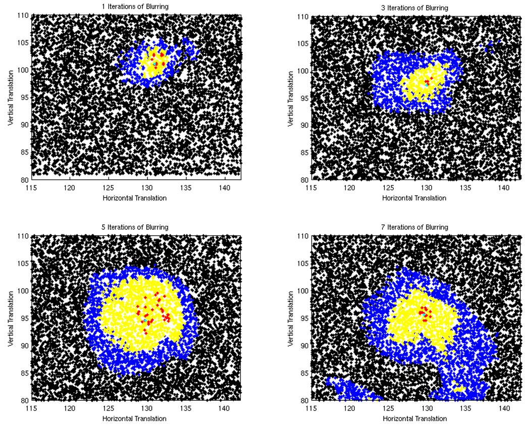
Figure 4 plots the 16,000 MCMC samples visited after burn-in for one, three, five, and seven iterations of blurring using the IP image model; samples for which χ_0.01(.), χ_0.05(.), and χ_0.1(.) equal 1 are colored red, yellow, and blue respectively. A multivariate normal proposal distribution was used as our MCMC proposal distribution. Of the 20,000 iterations, approximately 4,000 were discarded as burn-in states. Visual inspection of the expectations as a function of sample number confirmed that the Markov chain appeared to reach the stationary distribution after the 4000th iteration (Figure 3).

Fig. 4.

These figures show how the regions where χ_0.01(.) = 1 (red), χ_0.05(.) = 1 (yellow) and χ_0.1(.) = 1 (blue) grow as the image blurring increases. This example was made with the IP image model, and the ITK ellipse shape model.

Fig. 3.

The estimate of E[g(θ)] is plotted as a function of MCMC sample number for one example image. The green line shows the sample at which burn-in was stopped. The calm behavior of the chain after burn-in indicates that the chain has converged.

Figure 4 shows that as the amount of blurring increases the regions in the parameter space for which χ_0.05(.) = 1 and χ_0.1(.) = 1 grow in size. This agrees with our intuitive understanding of how the brain-skull boundary is blurred by gaussian smoothing.

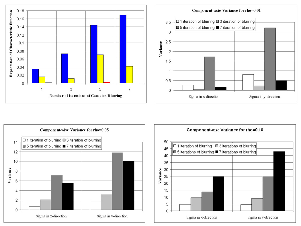
The measure E[χ_ρ(.)] did not always increase with the amount of blurring due to its inadequacy as a simple volume measure. E[χ_ρ(.)] only gives information about the size of the region for which χ_ρ(.) = 1, not its shape. For example, figure 5 reports a higher E[χ_0.05(.)] for 5 iterations of blurring than 7. However, the χ_0.05(.) = 1 region for the 7 iteration case is more spatially elongated in the x direction than in the 5 iteration case. Because the range of plausible x values is higher in the 7 iteration case, the 7 iteration delineation could be considered more uncertain than its 5 iteration counterpart. To capture this behavior, we computed the component-wise variance of the parameter values over the samples in each of the regions of Figure 4. If we denote the j^th component of the parameter vector θ by θj and the variance of a data set, S, by σ_S, then computing σ_Sj where S_j = {θ_j |χ_ρ(θ_j) = 1} for a pre-defined ρ will be a measure of the dispersion of the parameter values that are in the region defined by χ_ρ(θ) = 1.

Fig. 5.

Variance in the x- and y-directions for each of the colored regions shown in figure 4. Notice that the variance in the most blurred image is very large when ρ = 0.10, this implies a lack of precision.

The results from computing σ_Sj when ρ equals 0.01, 0.05 and 0.10 are given in figure 5. These plots capture the shape differences remarked on earlier. Thus, by combining the volumes and shapes of regions in the space of shape parameters, we detect the relative precision of the delineations.

4.4 Real 2D Data with Expert Uncertainty Ratings

The second test set consisted of 19 images selected out of the roughly 600 ADC images that have been analyzed to date by expert human raters who used standardized protocols to manually trace the brain and hippocampus. Of these, 5 images were considered normal by the raters, 5 were annotated as moderately poor– having either moderately poor image quality or large pathological features present– and 9 were extremely poor, with either extremely low image quality, or simultaneous low image quality and large pathologies. These labels provide qualitative expert ground truth about image quality that should be reflected in the uncertainty measures. All expert annotations were made prior to the development of our method.

In the first stage of our analysis, we use the uncertainty measures to detect any brain delineations that are probably inaccurate. We do this by computing a quantity, β, which is the proportion of MCMC samples θ with P(θ|I) > P(θ̂|I) If β is large, the automated segmentation method must have failed because its θ do not even correspond to a local maximum of P(θ|I).

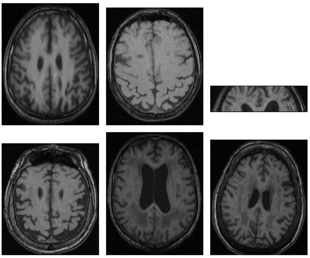
Of the 19 images, 11 had β values greater than 0.10 using the IP image model; only two had β values greater than 0.10 for the MSPSM image model. These were considered inaccurately segmented. Of the 11 removed by the IP image model, 5 were from the abnormal group. 6 of the excluded images are shown in figure 6.

Fig. 6.

The images shown in a − e were all initially labeled as abnormal images. The image is subfigure c is truly just a fraction of an image; we added it to the abnormal test set to see if the method could detect such a problem in an image. It is unclear why image f was inaccurately segmented.

Figure 7 shows the χ_ρ results for both segmentation methods tested. Expectations of χ_0.01(.) (red), χ_0.05(.) (yellow) and χ_0.1(.) (blue) are shown as colored bars. The first 4 images were labeled as normal; The next five were moderately poor; and the last four were extremely poor. Good and poor images provide similar uncertainty measures for MSPSM, suggesting that its image model is so over-simplified that it cannot to provide a precise delineation in any image; intuitively, the more complex IP model generally provided higher uncertainty estimates for the poor images (note, however, image 3). However, the IP model, with its more difficult task of optimizing more run-time parameters, is more prone to local minima as suggested by the larger number of discarded, high-β images. The high uncertainty of image 3 under the IP model may be due to an inadequacy in the expressive power of the IP model.

Fig. 7.

Uncertainty estimations made on the back end of the MSPSM and IP segmentation methods. Missing data represents an image with β > 0.10.

5 Discussion

In this paper we showed how MCMC methods can be used to sample the posterior distribution of an automated brain region delineation method for quantitative measurement of the uncertainty in a region-delineating surface. The method reported increasing brain region uncertainty as the blurring of a typical brain image increased; it also provided uncertainty measures that agreed well well qualitative expert ratings of image quality. By testing the method on a pair of image models we demonstrated that it is general enough to be used on the back end of a wide variety of current region delineation methods.

Future work will apply the method to other brain regions, including the hippocampus, and other automated segmentation methods. Methodologically, we will also explore novel modifications to the current method to increase sampling efficiency. Finally, we will explore the potential downstream uses of brain region uncertainty beyond detecting low-quality imaging data. For example, statistical analyses that relate brain region volume to clinical variables could use the uncertainty measures to down-weight region volumes derived from uncertain measurements.

References

- 1.Dellaert F, Seitz SM, Thorpe CE, Thrun S. Structure from motion without correspondence. IEEE Computer Society Conference on Computer Vision and Pattern Recognition (CVPR 2000) 2000;vol. 2 [Google Scholar]
- 2.Ford EB. Quantifying the uncertainty in the orbits of extrasolar planets. Astronomical Journal. 2005;129:1706. [Google Scholar]
- 3.Fox D, Burgard W, Dellaert F, Thrun S. Monte carlo localization: Efficient position estimation for mobile robots. Proceedings of the Sixteenth National Conference on Artificial Intelligence (AAAI 1999) 1999 [Google Scholar]
- 4.Isard M, Blake A. Contour tracking by stochastic propagation of conditional density. In: Buxton BF, Cipolla R, editors. ECCV 1996. LNCS. vol. 1064. Heidelberg: Springer; 1996. pp. 343–356. [Google Scholar]
- 5.Kelemen A, Szekely G, Gerig G. Elastic model-based segmentation of 3-d neuroradiological data sets. IEEE Transactions on Medical Imaging. 1999;18(10):828–839. doi: 10.1109/42.811260. [DOI] [PubMed] [Google Scholar]
- 6.Kuczera G, Parent E. Monte carlo assessment of parameter uncertainty in conceptual catchment models: the metropolis algortihm. Journal of Hydrology. 1998;211:69–85. [Google Scholar]
- 7.Visser SPJ. Medial temporal lobe atrophy and memory dysfunction as predictors for dementia in subjects with mild cognitive impairment. Journal of Neurology. 1999;246(6):477–485. doi: 10.1007/s004150050387. [DOI] [PubMed] [Google Scholar]
- 8.Harper BRR. Reporting of precision of estimates for diagnostic accuracy: a review. BMJ. 1999;318(1):1322–1323. doi: 10.1136/bmj.318.7194.1322. [DOI] [PMC free article] [PubMed] [Google Scholar]
- 9.Schreiber K, Sorensen PS, Koch-Henriksen N, Wagner A, Blinkenberg M, Svarer C, Petersen HC. Correlations of brain MRI parameters to disability in multiple sclerosis. 2001;104(1):24–30. doi: 10.1034/j.1600-0404.2001.00041.x. [DOI] [PubMed] [Google Scholar]
- 10.Smith S. Fast robust automated brain extraction. Human Brain Mapping. 2002;17(3):143–155. doi: 10.1002/hbm.10062. [DOI] [PMC free article] [PubMed] [Google Scholar]
- 11.Tu Z, Zhu SC. Image segmentation by data-driven markov chain monte carlo. IEEE Transactions on Pattern Analysis and Machine Intelligence. 2002;24(5):657–673. [Google Scholar]
- 12.Warfield SK, Zou KH, Wells WM. Simultaneous truth and performance level estimation (staple): an algorithm for the validation of image segmentation. IEEE Medical Imaging. 2004;23:903–921. doi: 10.1109/TMI.2004.828354. [DOI] [PMC free article] [PubMed] [Google Scholar]