An optimized blockwise nonlocal means denoising filter for 3-D magnetic resonance images

Abstract

A critical issue in image restoration is the problem of noise removal while keeping the integrity of relevant image information. Denoising is a crucial step to increase image quality and to improve the performance of all the tasks needed for quantitative imaging analysis. The method proposed in this paper is based on a 3D optimized blockwise version of the Non Local (NL) means filter [1]. The NL-means filter uses the redundancy of information in the image under study to remove the noise. The performance of the NL-means filter has been already demonstrated for 2D images, but reducing the computational burden is a critical aspect to extend the method to 3D images. To overcome this problem, we propose improvements to reduce the computational complexity. These different improvements allow to drastically divide the computational time while preserving the performances of the NL-means filter. A fully-automated and optimized version of the NL-means filter is then presented. Our contributions to the NL-means filter are: (a) an automatic tuning of the smoothing parameter, (b) a selection of the most relevant voxels, (c) a blockwise implementation and (d) a parallelized computation. Quantitative validation was carried out on synthetic datasets generated with BrainWeb [2]. The results show that our optimized NL-means filter outperforms the classical implementation of the NL-means filter, as well as two other classical denoising methods (Anisotropic Diffusion [3] and Total Variation minimization process [4]) in terms of accuracy (measured by the Peak Signal to Noise Ratio) with low computation time. Finally, qualitative results on real data are presented.

I. Introduction

Quantitative imaging involves image processing workflows (registration, segmentation, visualization, etc.) with increasing complexity and sensitivity to possible image artifacts. As a consequence, image processing procedures often require to remove image artifacts beforehand in order to make quantitative post-processing more robust and efficient. A critical issue concerns the problem of noise removal while keeping the integrity of relevant image information. This is particularly true for ultrasound images or magnetic resonance images (MRI) in presence of small structures with signals barely detectable above the noise level. In addition, a constant evolution of quantitative medical imaging is to process always larger cohorts of 3D data in order to find significant discriminants for a given pathology (e.g. see [5]). In this context, complex automatic image processing workflows are required [6] since human interpretation of images is no longer feasible. For effectiveness, these workflows have to be robust to a wide range of image qualities and parameter-free (or at least using auto-tuned parameters). This paper focuses on these critical aspects by introducing a new restoration scheme in the context of 3D medical imaging. The Non Local (NL-) means filter was originally introduced by Buades et al. [1] for 2D image denoising. The adaptation of this filter we propose for 3D images is based on (a) an automatic tuning of the smoothing parameter, (b) a selection of the most relevant voxels for the NL-means computation, (c) a blockwise implementation and (d) a parallelized computation. These different contributions allow to make the adapted filter fully-automated and above all to overcome the main limitation of the classical NL-means: the computational burden.

Section II gives a short overview of the literature on image restoration. Section III presents the proposed method with details about our contributions. Sections IV, V and VI show (a) the impact of our adaptations compared to the classical NL-means implementation and (b) a comparison with respect to other well established denoising methods on Gaussian and Rician noise. Both validation experiments are performed on a phantom data set in a quantitative way. Section VII shows results on real data such as 3 Tesla T1-weighted (T1-w) MRI and T2-weighted (T2-w) MRI of a patient with Multiple Sclerosis (MS) lesions. In section VIII we propose a discussion on the applicability and the further improvements of the NL-means filter in the context of 3D medical imaging.

II. State-of-the-ART

A. General overview

Many methods have been proposed for edge-preserving image denoising. Some popular approaches include Bayesian approaches [7], PDE-based approaches [3], [4], [8], [9], robust and regression estimation [10], adaptive smoothing [11], wavelet-based methods [12]–[14], bilateral filtering [15]–[17], local mode filtering [18], hybrid approaches [19]–[21].

Strong theoretical links exist between most of these techniques, as recently shown for local mode filtering [18], bilateral filtering, anisotropic diffusion and robust estimation [17], [22] and adaptive smoothing [23], anisotropic diffusion and total variation minimization scheme [24].

More recently, some promising methods have been proposed for improved image denoising, based on statistical averaging schemes enhanced via incorporating a variable spatial neighborhood scheme [25]–[29]. Other approaches consist in modeling non-local pairwise interactions from training data [30] or a library of natural image patches [31], [32]. The idea is to improve the traditional Markov random field (MRF) models by learning potential functions from examples and extended neighborhoods for computer vision applications [30]–[32]. Awate and Whitaker proposed another non-parametric patch-based method relying on comparisons between probability density functions [33].

Some of these techniques, generally developed for 2D images, have often been extended to 3D medical data, especially to MR images: anisotropic diffusion [34], [35], total variation [36], bilateral filtering and variants [37], wavelet-based filtering [38]–[42], hybrid approaches [43], [44].

B. Introduction of the NL-means filter

Most of the denoising methods restore the intensity value of each image voxel by averaging in some way the intensities of its (spatially) neighboring voxels. The basic and intuitive approach is to replace the value of the voxel by the average of the voxels in its neigbourhood (so-called box filtering [45]). In practice, this filter has been shown to be outperformed by the Gaussian filter, which consists in weighting each voxel in the neighborhood according to its distance to the voxel under study. Both filters can be iterated until the desired amount of smoothing is reached. Such data-independent approaches can be implemented very efficiently. Their major drawback is that they blur the structures of interest in the image (e.g. edges or small structures and textures).

This has naturally led to data-dependent approaches, which aim at eliminating (or reducing the influence of) the neighboring voxels dissimilar to the voxel under study. Simple order statistic operators can be used for this purpose, such as the median filter, leading to a simple generalization of the box filter. More sophisticated approaches, based on image derivatives have been successfully proposed for many applications, such as adaptive smoothing [11] and anisotropic diffusion [3]. Neighborhood filters [46], [47] and variants [15], [16], have been also proposed and consist in averaging input data over the image voxels that are spatially close to the voxel under study and with similar gray-level values.

All these techniques rely on the idea that the restored value of a voxel should only depend on the voxels in its spatial neighborhood that belong to the same population, that is the same image context. This has been termed by Michael Elad as the locally adaptive recovery paradigm [17]. Another approach has been recently proposed, that has shown very promising results. It is based on the idea that any natural image has redundancy, and that any voxel of the image has similar voxels that are not necessarily located in a spatial neighborhood. First introduced by Buades et al. in [1], the NL-means filter is based on this redundancy property of periodic images, textured images or natural images to remove noise. In this approach, the weight involving voxels in the average, does not depend on their spatial proximity to the current voxel but is based on the intensity similarity of their neighborhoods with the neighborhood of the voxel under study, as in patched-based approaches. In other words, the NL-means filter can be viewed as an extreme case of neighborhood filters with infinite spatial kernel and where the similarity of the neighborhood intensities is substituted to the point-wise similarity of gray levels as in commonly-used bilateral filtering. This new non-local recovery paradigm allows to combine the two most important attributes of a denoising algorithm: edge preservation and noise removal.

III. Methods

In the following, we introduce the notations:

• u : Ω³ ↦ ℝ is the image, where Ω³ represents the grid of the image, considered as cubic for the sake of simplicity and without loss of generality (|Ω³| = N³).

• for the original voxelwise NL-means approach

  • – u(x_i) is the intensity observed at voxel x_i.

  • – V_i is the cubic search volume centered on voxel x_i of size |V_i| = (2M + 1)³, M ∈ ℕ.

  • – N_i is the cubic local neighborhood of x_i of size |N_i| = (2d + 1)³, d ∈ ℕ.

  • – u(N_i) = (u⁽¹⁾(N_i), …, u^(|N_i|)(N_i))^T is the vector containing the intensities of N_i.

  • – NL(u)(x_i) is the restored value of voxel x_i.

  • – w(x_i, x_j) is the weight of voxel x_j when restoring u(x_i).

• for the blockwise NL-means approach

  • – B_i is the block centered on x_i of size |B_i| = (2α + 1)³, α ∈ ℕ.

  • – u(B_i) is the vector containing the intensities of the block B_i.

  • – NL(u)(B_i) is the vector containing the restored value of B_i.

  • – w(B_i, B_j) is the weight of block B_j when restoring the block u(B_i).

  • – the blocks B_ik are centered on voxels x_ik with i_k = (k₁n, k₂n, k₃n), (k₁, k₂, k₃) ∈ ℕ³ and n represents the distance between the centers of the blocks B_ik.

A. The Non Local means filter

In the classical formulation of the NL-means filter, the restored intensity NL(u)(x_i) of the voxel x_i, is the weighted average of all the voxel intensities in the image u defined as:

$$NL(u)(x_i)=\sum _{x_j\in {\mathrm{\Omega }}^3}w(x_i,x_j)u(x_j)$$ (1)

where u(x_j) is the intensity of voxel x_j and w(x_i, x_j) is the weight assigned to u(x_j) in the restoration of voxel x_i. More precisely, the weight quantifies the similarity of the local neighborhoods N_i and N_j of the voxels x_i and x_j under the assumptions that w(x_i, x_j) ∈ [0, 1] and Σ_{xj∈ Ω³} w(x_i, x_j) = 1 (cf Fig. 1 left). The classical definition of the NL-means filter considers that each voxel can be linked to all the others, but for practical computational reasons the number of voxels taken into account in the weighted average can be limited to the so-called “search volume” V_i of size (2M+1)³, centered at the current voxel x_i.

Fig. 1.

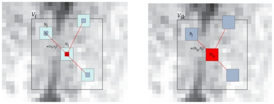
Left: Classical voxelwise NL-means filter: 2D illustration of the NL-means principle. The restored value of voxel x_i (in red) is the weighted average of all intensities of voxels x_j in the search volume V_i, based on the similarity of their intensity neighborhoods u(N_i) and u(N_j). In this example, we set d = 1 and M = 8. Right: Blockwise NL-means filter: 2D illustration of the blockwise NL-means principle. The restored value of the block B_ik is the weighted average of all the blocks B_j in the search volume V_ik. In this example, we set α = 1 and M = 8.

For each voxel x_j in V_i, the Gaussian-weighted Euclidean distance ${\parallel ·\parallel }_{2,a}^2$ defined in [1], is computed between u(N_j) and u(N_i). This distance is a classical L₂ norm convolved with a Gaussian kernel of standard deviation a, and measures the distance between neighborhood intensities. Given this distance, w(x_i, x_j) is computed as follows:

$$w(x_i,x_j)=\frac{1}{Z_i}{e}^{-\frac{{\parallel \mathbf{u}(N_i)-\mathbf{u}(N_j)\parallel }_{2,a}^2}{h^2}}$$ (2)

where Z_i is a normalization constant ensuring that Σ_j w(x_i, x_j) = 1, and h acts as a smoothing parameter controlling the decay of the exponential function. When h is very high, all the voxels x_j in V_i will have the same weight w(x_i, x_j) with respect to the voxel x_i. The restored value NL(u)(x_i) will be then approximately the average of the intensity values of the voxels in V_i leading to strong smoothing of the image. When h is very low, the decay of the exponential function will be strong, thus only few voxels x_j in V_i with u(N_j) very similar to u(N_j) will have a significant weight. The restored value NL(u)(x_i) will tend to be the weighted average of some voxels with a similar neighborhood to current voxel x_i leading to a weak smoothing of the image. In Section III-B.1, a trade-off has then to be found, and we propose a method to automatically estimate the optimal value of h.

In [1], Buades et al. show that, for 2D natural images, the NL-means filter outperforms state-of-the-art denoising methods such as the Rudin-Osher-Fatemi Total Variation minimization scheme [4], the Perona-Malik Anisotropic diffusion [3] or translation invariant wavelet thresholding [48]. Nevertheless, the main drawback of the NL-means filter is the computational burden due to its complexity, especially for 3D images. Indeed, for each voxel of the volume, distances between the intensity neighborhoods u(N_i) and u(N_j) for all the voxels x_j contained in V_i need to be computed. Let N³ denote the size of the 3D image, then the complexity of the filter is in the order of ((N(2M+1)(2d+1))³). For a 3D MRI of size 181 × 217 × 181 with the smallest possible value for d and M (d = 1 and M = 5), the computational time reaches up to 6 hours on 3 GHz CPU. This time is far beyond a reasonable duration expected for a denoising filter in a medical practice. For this reason, we propose several adaptations to reduce the computational burden which are detailed in Section III-B. We also show that these adaptations improve the quality of the denoising compared to the classical implementation.

B. Improvements of the NL-means filter

1. Automatic tuning of the Smoothing parameter h

According to [1], the smoothing parameter h depends on the standard deviation of the noise σ, and typically a good choice for 2D images is h ≈ 10σ. Equation 2 shows that h also needs to take into account |N_i|, if we want a filter independent of the neighborhood size. Indeed, the L₂ norm increasing with |N_i|, h needs also to be increased to obtain an equivalent filter. The automatic tuning of the smoothing parameter h comes to determine the relationship h² = f(σ², |N_i|, β) where β is a constant. Let us show how we can estimate this relationship:

1. In case of an additive white Gaussian noise, the standard deviation of noise can be estimated via pseudo-residuals ε_i as defined in [49], [50]. For each voxel x_i of the volume Ω³, let us define:

   $${\epsilon }_i=\sqrt{\frac{6}{7}}\left(u(x_i)-\frac{1}{6}\sum _{x_j\in P_i}u(x_j)\right)$$ (3)

   P_i being the 6-neighborhood at voxel x_i and the constant $\sqrt{6/7}$ is used to ensure that $\mathbb{E}[{\epsilon }_i^2]={\widehat{\sigma }}^2$ in homogeneous areas. Thus, the standard deviation of noise σ̂ is computed as the least square estimator:

   $${\widehat{\sigma }}^2=\frac{1}{\mid {\mathrm{\Omega }}^3\mid }\sum _{i\in {\mathrm{\Omega }}^3}{\epsilon }_i^2$$ (4)

2. Initially, the NL-means filter was defined with a Gaussian-weighted Euclidean distance, ${\parallel ·\parallel }_{2,a}^2$ defined in [1]. However, in order to make the filter independent of |N_i|, to simplify the complexity of the problem, and to reduce the computational time, we used the classical Euclidean distance ${\parallel ·\parallel }_2^2$ normalized by the number of elements:

   $$\frac{1}{\mid N_i\mid }{\parallel \mathbf{u}(N_i)-\mathbf{u}(N_j)\parallel }_2^2=\frac{1}{\mid N_i\mid }\sum _{p=1}^{\mid N_i\mid }{(u^{(p)}(N_i)-u^{(p)}(N_j))}^2.$$ (5)

   Finally, Equation 2 becomes:

   $$w(x_i,x_j)=\frac{1}{Z_i}{e}^{-\frac{{\parallel \mathbf{u}(N_i)-\mathbf{u}(N_j)\parallel }_2^2}{2\beta {\widehat{\sigma }}^2\mid N_i\mid }}$$ (6)

   where only the adjusting constant β needs to be manually tuned. In the case of Gaussian noise, β is theoretically be close to 1 (see [51] p. 21 for theoretical justification) if the estimation σ̂ of the standard deviation of the noise is correct. The adjustment of β will be discussed in section V-A.

2. Voxel selection in the search volume

To deal with computational burden, Mahmoudi and Sapiro [52] recently proposed a method to preselect a subset of the most relevant voxels x_j in V_i to avoid useless weight computations. In other words, the main idea is to select only the voxels x_j in V_i that will have the highest weights w(x_i, x_j) in Equation 1 without having to compute all the Euclidean distances between u(N_i) and u(N_j). A priori neglecting the voxels which are expected to have small weights tends to speed up the filter and to improve the results (see Table II). In [52], this selection is based on the similarity of the mean value of u(N_i) and u(N_j), and on the similarity of the average over the neighborhoods N_i and N_j of the gradient orientation at pixel x_i and x_j. Intuitively, similar neighborhoods have the same mean and the same gradient orientation. The computation of the gradient orientation is very sensitive to noise and thus requires robust estimation techniques. This is too computationally expensive for medical applications. For this reason, in our implementation, the preselection of voxels in V_i is based on the mean and the variance of u(N_i) and u(N_j) which allows to decrease the computational burden. Figure 2 shows that the maps of local means and local variances are simple estimators allowing to discriminate different tissue classes and edges in images. In this way, the maps of local means and local variances are precomputed in order to avoid repetitive calculations for the same neighborhood. The selection tests can be expressed as follows:

$$w(x_i,x_j)=\{\begin{array}{ll}\frac{1}{Z_i}{e}^{-\frac{{\parallel \mathbf{u}(N_i)-\mathbf{u}(N_j)\parallel }_2^2}{2\beta {\widehat{\sigma }}^2\mid N_i\mid }}\hfill & \text{if}{\mu }_1<\frac{\overline{\mathbf{u}(N_i)}}{\overline{\mathbf{u}(N_j)}}<\frac{1}{{\mu }_1}\text{and}{\sigma }_1^2<\frac{\text{Var}(\mathbf{u}(N_i))}{\text{Var}(\mathbf{u}(N_j))}<\frac{1}{{\sigma }_1^2}\hfill \\ 0\hfill & \text{otherwise}.\hfill \end{array}$$ (7)

where $\overline{\mathbf{u}(N_i)}$ and Var(u(N_i)) represents respectively the mean and the variance of the local neighborhood N_i of voxel x_i. As suggested in [52], with this kind of selection, the NL-means filter tends to better preserve the detailed regions while slightly spoiling the denoising of the flat regions. Indeed, in flat regions increasing the number of voxels tends to improve denoising because there are a large number of similar voxels. In more cluttered regions, increasing the number of voxels tends to remove the details during smoothing because there are very few similar voxels.

TABLE II. Comparison of different implementations of the NL-means filters in terms of computational time and denoising quality.

The time is obtained with multithreading on 8 CPUs at 3GHZ and Intel(R) Pentium(R) D CPU 3.40GHZ and without multithreading on 1 CPU at 3GHZ. These results are obtained on a T1-w BrainWeb image with 9% of Gaussian noise (σ = 13.5). The parameters used are the default parameters. The average number of voxels/blocks used in V_i to denoise u(x_i) shows the impact of voxels/blocks selection. For the non-optimized implementations all the voxels/blocks in V_i are taken into account to denoise u(x_i). Thus, the number of voxels/blocks used are |V_i| = (2M + 1)³ = 11³. For the optimized implementations the voxel selection allows to drastically reduce this number.

Gaussian Noise	Computational time (in s)			PSNR (in dB)	Average number of voxels/blocks used in Vi to denoise xi
	Xeon 3GHz	8 × Xeon 3GHz	DualCore 3.40 GHz
NL-means	21790	2780	4208	32.59	113 = 1331 voxels
Blockwise NL-means	1800	251	734	31.73	113 = 1331 blocks
Optimized NL-means	3169	436	778	34.44	174.8 voxels
Optimized Blockwise NL-means	328	63	135	33.75	174.8 blocks

Fig. 2.

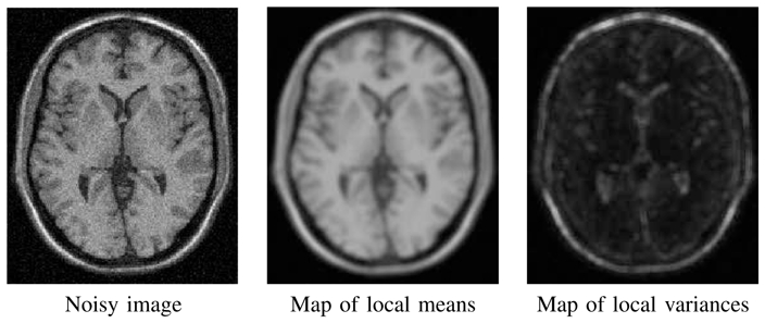
Left: noisy image with 9 % of Gaussian noise (see Section IV). Center: map of the mean of u(N_i) denoted $\overline{\mathbf{u}(N_i)}$. Right map of the variance of u(N_i) denoted Var(u(N_i)). In these examples, we set N_i = 5 × 5 × 5 voxels.

3. Blockwise implementation

A blockwise implementation of the NL-means is developed as suggested in [1]. This approach consists in a) dividing the volume into blocks with overlapping supports, b) performing NL-means-like restoration of these blocks and c) restoring the voxels values based on the restored values of the blocks they belong to.

1. A partition of the volume Ω³ into overlapping blocks B_ik of size (2α + 1)³ is performed, such as Ω³ = ∪_k B_ik, under the constraint that the intersections between the B_ik are non-empty (see Fig 3). These blocks are centered on voxels x_ikwhich constitute a subset of Ω³. The x_ik are equally distributed at positions i_k = (k₁n, k₂n, k₃n), (k₁, k₂, k₃) ∈ ℕ³ where n represents the distance between the centers of B_ik. To ensure a global continuity in the denoised image, the support overlapping of blocks has to be non empty: 2α > n.

2. For each block B_ik, a NL-means-like restoration is performed as follows:

   $$\mathbf{NL}(u)(B_{i_k})=\sum _{B_j\in V_{i_k}}w(B_{i_k},B_j)\mathbf{u}(B_j)$$ (8)

   with

   $$w(B_{i_k},B_j)=\frac{1}{Z_{i_k}}{e}^{-\frac{{\parallel \mathbf{u}(B_{i_k})-\mathbf{u}(B_j)\parallel }_2^2}{2\beta {\widehat{\sigma }}^2\mid N_i\mid }}$$ (9)

   where Z_ik is a normalization constant ensuring that Σ_{Bj∈ Vik} w(B_ik, B_j) = 1 (see Fig. 1 (right)).

3. For a voxel x_i included in several blocks B_ik, several estimations of the restored intensity NL(u)(x_i) are obtained in different NL(u)(B_ik) (see Fig 3). The estimations given by different NL(u)(B_ik) for a voxel x_i are stored in a vector A_i. The final restored intensity of voxel x_i is then defined as:

   $$NL(u)(x_i)=\frac{1}{\mid {\mathbf{A}}_i\mid }\sum _{p\in {\mathbf{A}}_i}{\mathbf{A}}_i(p).$$ (10)

Fig. 3. Blockwise NL-means Filter.

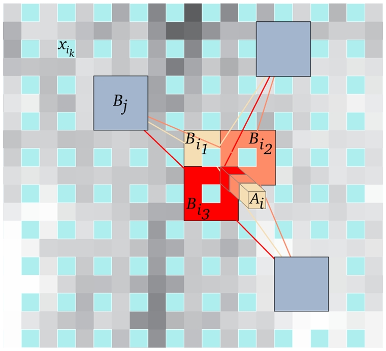
For each block B_ikcentered on voxel x_ik, a NL-means like restoration is performed from blocks B_j. In this way, for a voxel x_i included in several blocks, several estimations are obtained. The restored value of voxel x_i is the average of the different estimations stored in vector A_i. In this example α = 1, n = 2 and |A_i| = 3.

The main advantage of this approach is to significantly reduce the complexity of the algorithm. Indeed, for a volume Ω³ of size N³, the global complexity is $\mathcal{O}({(2\alpha +1)}^3{(2M+1)}^3{(\frac{N-n}{n})}^3)$. For instance, with n = 2, the complexity is divided by a factor 8. The voxels selection principle can also be applied to the blockwise implementation:

$$w(B_{i_k},B_j)=\{\begin{array}{ll}\frac{1}{Z_{i_k}}{e}^{-\frac{{\parallel \mathbf{u}(B_{i_k})-\mathbf{u}(B_j)\parallel }_2^2}{2\beta {\widehat{\sigma }}^2\mid N_i\mid }}\hfill & \text{if}{\mu }_1<\frac{\overline{\mathbf{u}(B_{i_k})}}{\overline{\mathbf{u}(B_j)}}<\frac{1}{{\mu }_1}\text{and}{\sigma }_1^2<\frac{\text{Var}(\mathbf{u}(B_{i_k}))}{\text{Var}(\mathbf{u}(B_j))}<\frac{1}{{\sigma }_1^2}\hfill \\ 0\hfill & \text{otherwise}.\hfill \end{array}$$ (11)

where $\overline{\mathbf{u}(B_{i_k})}$ and Var(u(B_ik)) represent respectively the mean and the variance of the intensity function, for the block B_ik centered on the voxel x_ik.

4. Parallel computation

Another way to reduce the computational time is to distribute the operations on several processors via a cluster or a grid. The intrinsic nature of the NL-means filter makes it perfectly suited for parallelization and multithreading implementation. One of the main advantage of this filter, when compared to others method such as Anisotropic Diffusion or Total Variation minimization, is that the operations are performed without any iterative schemes. Thus, the parallelization of the NL-means filter is straightforward to perform and very efficient. We divide the volume into sub-volumes, each of them being treated separately by one processor. A server with 8 Xeon processors at 3 GHz and a Intel(R) Pentium(R) D CPU 3.40GHz were used in our experiments.

IV. Materials

A. The BrainWeb Database

In order to evaluate the performances of the NL-means filter on 3D MR images, tests were performed on the BrainWeb database¹ [2]. Two images were simulated: T1-w MR image using SFLASH sequence (volume size = 181 × 217 × 181) and T2-w MR image with MS from SFLASH sequence (volume size = 181 × 217 × 181). As reported previously, it is a known fact that the MR images are corrupted by a Rician noise [53], [54], which can be well approximated by a white Gaussian noise in high intensity areas, typically in brain tissues [38]. In order to verify if this approximation can be used for a NL-means based denoising, experiments are performed on phantom images with Gaussian and Rician noise.

1. Gaussian Noise

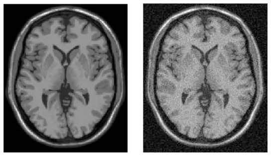
A white Gaussian noise was added on the “ground truth”, and the notations of BrainWeb are used: a noise of 3% is equivalent to $\mathcal{N}(0,\nu \frac{3}{100})$, where ν is the value of the brightest tissue in the image (150 for T1-w and 250 for T2-w). Several images were simulated to validate the performances of the denoising on various images (see Fig. 4):

Fig. 4. Synthetic data used for validation with Gaussian Nnoise.

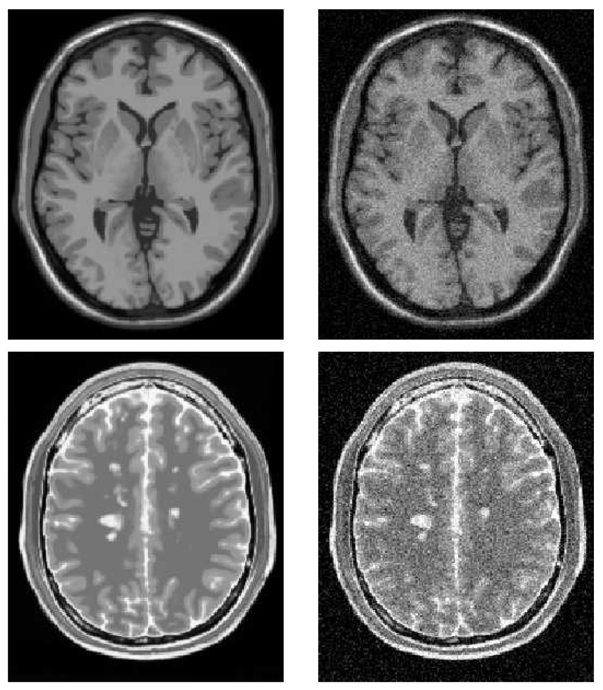
Example of the Brainweb Database. Top: T1-w images without any noise (left), and corrupted with a white Gaussian noise at 9% (right). Bottom: T2-w images with MS lesions without noise (left), and corrupted with a white Gaussian noise at 9% (right).

• T1-w MR images for 4 levels of noise 3%, 9%, 15% and 21%.

• T2-w MR images with Multiple Sclerosis (MS) lesions for 4 levels of noise 3%, 9%, 15% and 21%.

T2-w images were used in order to show that our approach and its calibration are not specific to T1-w MRI sequences. Moreover, the tests on T2-w MRI with MS show how the NL-means filter could be useful in a pathological context due to its preservation of anatomic and pathologic structures.

2. Rician Noise

The Rician noise was build from white Gaussian noise in the complex domain. Firstly, two images are computed:

• I_r(x_i) = I₀(x_i) + η₁(x_i), η₁(x_i) ~ (0, σ)

• I_i(x_i) = η₂(x_i), η₂(x_i) ~ (0, σ)

where I₀ is the “ground truth” and σ is the standard deviation of the added white Gaussian noise. Then, the noisy image is computed as:

$$I_N(x_i)=\sqrt{I_r{(x_i)}^2+I_i{(x_i)}^2}$$ (12)

The notation 3% for the Rician noise means that the Gaussian noise used in complex domain is equivalent to $\mathcal{N}(0,\nu \frac{3}{100})$, where ν is the value of the brightest tissue in the image (150 for T1-w). According to the Peak Signal to Noise Ratio (PSNR) (see Eq. 13) between “ground truth” and noisy images, for a same level of noise, the Rician noise is stronger than the Gaussian noise (see Tab. I). Several images were simulated (see Fig. 5):

Fig. 5. Synthetic data used for validation with Rician noise.

Example of the Brainweb Database. T1-w images without any noise (left), and corrupted with a Rician noise at 9% (right).

• T1-w MR images for 4 levels of noise 3%, 9%, 15% and 21%.

B. Real Data

1. T1-w high field MRI Data

To show the efficiency of the NL-means filter on real data, tests were performed on image acquired with a high field MR system (Bruker 3 Tesla). The data used was a 256 × 256 × 256 T1-w image.

2. T2-w with Multiple Sclerosis lesions

In a pathological context, the denoising step is crucial especially when the structures of interest have a small size: the integrity of pathological structures must be preserved by the denoising method. As said earlier, one objective of denoising is to include such processing in complex medical imaging workflows. This kind of workflows is widely used to process large cohort of subjects in many neurological diseases such as MS lesions. The data used for MS lesions qualitative validation was a T2-w MR image from an axial dual-echo, turbo spin-echo sequence (Philips 1.5 Tesla).

V. Validation on a Phantom data set with added Gaussian Noise

In the following, let us define:

• NL-means is the standard voxelwise implementation with automatic tuning of the smoothing parameter.

• Optimized NL-means is a voxelwise implementation with automatic tuning of the smoothing parameter, voxel selection and multithreading.

• Blockwise NL-means is the standard blockwise implementation with automatic tuning of the smoothing parameter.

• Optimized Blockwise NL-means is a blockwise implementation with automatic tuning of the smoothing parameter, block selection and multithreading.

In this section different aspects of NL-means filter implementation were investigated. First, the impact of the automatic tuning of the filtering parameter (Section V-A) and the influence of the size of the search volume and the neighborhood were studied (Section V-B). Then, the impact of voxels selection and blockwise implementation is analyzed via the comparison of the NL-means, Optimized NL-means, Blockwise NL-means and Optimized Blockwise NL-means filters (Sections V-C and V-D). Finally, we compare the proposed Optimized Blockwise NL-means filter with other well-established denoising methods: Anisotropic Diffusion filter [3] (implemented in VTK²) and Rudin-Osher-Fatemi Total Variation (TV) minimization process [4] (3D extension of the Megawave 2 implementation³) (Section V-G). The different variants of the NL-means filter can be freely tested at: http://www.irisa.fr/visages/benchmarks

In the following, several criteria are used to quantify the performances of each method: the PSNR obtained for different noise levels, histogram comparisons between the denoised images and the “ground truth”, and finally visual assessment. For the sake of clarity, the PSNR and the histograms are estimated only in a region of interest obtained by removing the background. For 8-bit encoded images, the PSNR is defined as follows:

$$\mathit{PSNR}=20{log}_{10}\frac{255}{\mathit{RMSE}}$$ (13)

where the RMSE is the root mean square error estimated between the ground truth and the denoised image.

In this section, the central parameters of interest are:

• β defining the smoothing parameter h: h² = 2βσ̂²|N_i| (see section III-B.1).

• M related to |V_i|: |V_i| = (2M + 1)³.

• d related to |N_i|: |N_i| = (2d + 1)³.

• μ₁ and ${\sigma }_1^2$ corresponding to the thresholds involving in the voxel selection.

In each experiment (Sections V-A, V-B and V-C), we let one parameter vary while remaining the others constant, with default values: β = 1, M = 5, d = 1 and μ₁ = 0.95, ${\sigma }_1^2=0.5$. Concerning the blockwise implementation the default parameters are n = 2 and α = 1.

Our experiments have shown that all the versions of the NL-means filter (NL-means, Optimized NL-means, Blockwise NL-means and Optimized Blockwise NL-means) tend to have a similar behavior with respect to the variation of the parameters. In that context, all the results are displayed with the proposed Optimized Blockwise NL-means filter, even if equivalent conclusions can be drawn with the NL-means, Optimized NL-means and Blockwise NL-means filters.

Validation was performed on T1-w and T2-w MRI, but the results concerning the study of the parameter influences are shown for T1-w MRI only. The results on T2-w MRI are shown in section V-F in order to underline that the parameters calibrated for T1-w MRI work fine on T2-w MRI.

A. Influence of the automatic tuning of smoothing parameter h

Figure 6 shows the influence of the automatic determination of the smoothing parameter h² = 2βσ̂²|N_i|. As described in III-B.1, h is a function of the global standard deviation of the noise σ̂ in the volume esimated from pseudo-residuals (see 3 and Eq. 4). Here, β allows to adjust the automatic estimation of h in order to determine the optimal smoothing parameter 2βσ̂²|N_i| for each level of noise (see 6). For low levels of noise the best value of β is close to 0.5. For high levels of noise this value is 1. These results show that the estimation of the standard deviation of the noise is correctly performed by pseudo-residuals. These observations underline (a) how efficient the automatic estimation of the smoothing parameter h is, and (b) how the NL-means can be used without manual parameter tuning.

Fig. 6. Calibration of the smoothing parameter.

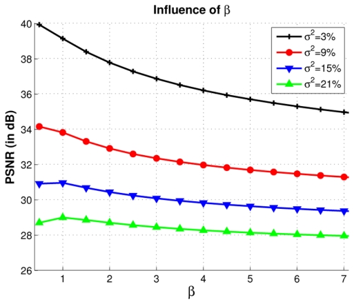
h: Influence of the smoothing parameter 2βσ̂²|N_i| on the PSNR, according to β and for several levels of noise. For low levels of noise the best value of β is close to 0.5. For high levels of noise this value is 1. The default value of β is set to 1, thus the estimation of h is h² = 2σ̂². These results are obtained with σ̂² = 3.42% at 3%, σ̂² = 7.93% at 9%, σ̂² = 12.72% at 15% and σ̂² = 17.44% at 21%.

B. Influence of the size of the search volume and the neighborhood

Figure 7 shows the influence of the size of the search volume and the local neighborhood. Increasing the number of voxels in the search volume V_i does not seem to affect the PSNR when M is greater than 5. Indeed, the theoretic definition of the NL-means filter states that the weighted average (see Eq. 1) computed for the restoration of voxel x_i should be performed on all voxels x_j ∈ Ω³. Practically, the limit M = 5 prevents useless computations. Moreover, increasing d degrades the denoising process. When d increases the NL-means filter drastically slows down. That is why we have not investigated the impact of d for d > 3.

Fig. 7. Influence of the size |V_i| = (2M + 1)³ and |N_i| = (2d + 1)³ for denoising.

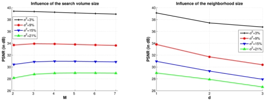
Influence of the size of the search volume and the size of the neighborhood on the PSNR, for several levels of noise. Left: Variation of the size M of the search volume V_i for d = 1. Right: Variation of the size d of the neighborhood N_i for M = 5. These results show that the limit M = 5 prevents useless computation. Moreover, increasing d degrades and drastically slows down the algorithm.

C. Influence of the voxel selection

The selection of the voxels in the search volume V_i is achieved by supposing that only the voxels whose the neighborhood is similar to the neighborhood of the voxel under study could be considered (see Eq. 1). To do so, as defined in III-B.2, the weight w(x_i, x_j) is calculated only for voxels such that: ${\mu }_1<\frac{\overline{\mathbf{u}(N_i)}}{\overline{\mathbf{u}(N_j)}}<\frac{1}{{\mu }_1}$ and ${\sigma }_1^2<\frac{\text{Var}(\mathbf{u}(N_i))}{\text{Var}(\mathbf{u}(N_j))}<\frac{1}{{\sigma }_1^2}$. The influence of the limits μ₁ and ${\sigma }_1^2$ is studied in Figure 8. In a first experiment μ₁ varies according to γ such as μ₁ = 1 − γ while ${\sigma }_1^2=0.5$. In a second experiment ${\sigma }_1^2$ varies according to γ following ${\sigma }_1^2=1-\gamma$ while μ₁ = 0.95.

Fig. 8. Influence of the limits of the voxels selection.

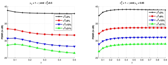
Influence of the limits μ₁ and ${\sigma }_1^2$ on the PSNR, for several level of noise. Left: ${\sigma }_1^2=0.5$, while μ₁ varies with γ. A restrictive selection based on the mean (low values of γ) increases the PSNR. The optimal limits are obtained for μ₁ = 0.95. Right: μ₁ = 0.95 and ${\sigma }_1^2$ varies accordingly to γ. A too restrictive selection (low values of γ) degrades the PSNR. In addition, a too permissive selection (high values of γ) does not increase the PSNR while concurrently increasing uselessly the computational burden. A good compromise is found by fixing ${\sigma }_1^2=0.5$.

Figure 8 (left) shows that a restrictive selection based on the mean (low values of γ) increases the PSNR. In other words, the number of voxels taken into account in the weighted average is drastically reduced, as well as the computational time (also see Tab. II). The optimal limits were obtained for μ₁ = 0.95 while ${\sigma }_1^2=0.5$. Concerning the variance (Figure 8, right), we observe that a too restrictive selection degrades the PSNR. In addition, a too permissive selection does not increase the PSNR while increasing uselessly the computational burden. A compromise was found by fixing ${\sigma }_1^2=0.5$. There is a clear dependency between the bounds for the mean and the variance. An optimal trade-off was determined experimentally.

D. Influence of the blockwise implementation

Tab. II shows that the blockwise approach of the NL-means filter, with and without voxels selection (see Eq. 11), allows to drastically reduce the computational time. With a distance between the block centers n = 2, the blockwise approach divides this time by a factor 2³ = 8 (see Tab. II). However, computational time reduction needs to be balanced with a slight decrease of the PSNR (see Fig. 9, left). For the optimized versions, the voxels/blocks selection in the search volume has several impacts. First, by reducing the average number of voxels/blocks used in the weighted averages, this decreases the computational time compared to the non-optimized versions (see Tab. II). Second, the selection of the most relevant voxels/blocks increases the quality of denoising for all the noise levels (see Fig. 9 (left) and Tab. II).

Fig. 9. Impact of the blockwise implementation and voxels selection.

Comparison of the different implementations of the NL-means filter, with α = 1. Left: on T1-w images. For the Optimized Blockwise NL-means filter, as for the Optimized NL-means filter, the selection of voxels/blocks in the search volume improves the quality of denoising and decreases the computational burden (see Tab. II). The reduction of computational time brought by the blockwise approach needs to be balanced with a slight decrease in quality of denoising. Right: on T2-w images with MS lesions. The same conclusions can be drawn for this kind of images. These results suggest that the parameters tuning determined experimentally on T1-w images are not T1-specific.

E. Multithreading

As described in section III-B.4, the multithreading in the case of the NL-means filter is particularly adapted due its non iterative nature. For the classical pixelwise NL-means implementation, the parallelization allows to divide the computational time by a factor close to the numbers of CPU. As eight processors were used for our experiments, the computational time with multithreading is about 8 times smaller (see Tab. II, $\frac{21790}{2780}=7.84$ and $\frac{3169}{436}=7.27$). For the blockwise implementations the speedup is less $\frac{1800}{251}=7.17$ and $\frac{328}{63}=5.37$). The difference of speedup between the classical NL-means and the blockwise NL-means filters have two origins.

• First, in blockwise version several threads could write at the same memory location (i.e. vector A_i) at the same time. In multi-treading programming this kind of possibilities requires a lock which protects the memory location during the writing. Unfortunately, to lock a memory location speeds down the computational process.

• Second, as the required computation time is shorter for the blockwise than for the voxelwise implementation, the relative contribution of the non-multithreaded operations in the overall computation time (opening and closing of file, computation of the local maps, etc.) is much higher in the blockwise compared to the voxelwise implementation. As a consequence, the speed-up factor will be higher in the latter

In order to underline that the utilization of 8-CPUs is not required by our filter, the denoising have been also performed on a more common architecture: a DualCore Intel(R) Pentium(R) D CPU 3.40GHz. The results show that our filter takes less than 3 minutes to denoise a volume 181 × 217 × 181 voxels on this architecture.

To conclude, the different improvements included in the proposed Optimized Blockwise NL-means filter (i.e., blockwise approach and blocks selection) allow to speed up the denoising procedure, compared to NL-means filter, by a factor of 66 on 1 Xeon at 3GHz, 44 on 8× Xeon at 3GHz and 31 on a DualCore at 3.40GHz.

F. Optimized Blockwise NL-means filter on T2-w MRI with MS

Figure 9 (right) presents the results obtained by the different NL-means filter versions on T2-w MRI with MS lesions. The optimal parameters (i.e. the default parameters described in section V), experimentally determined on T1-w MRI, and the automatic tuning of h were used on T2-w MRI. The Optimized NL-means and Optimized Blockwise NL-means filters outperform the NL-means and Blockwise NL-means filters also on T2-w MRI. The most important difference between the optimized and non-optimized versions are observed on T2-w MRI, which could be explained by the higher level of noise in the simulated T2-w MRI compared to T1- w MRI. Actually, the variance of noise varies with respect to the highest intensity tissues which is 150 in T1-w and 250 in T2-w. For 9% the variance of noise is 13.5 in T1-w images and is 22.5 in T2-w images because the highest tissue intensity is superior in T2-w images. These results suggest that the parameters experimentally tuned on T1-w images can be used for T2-w images. Figure 10 shows an example of denoising obtained by the optimized blockwise NL-means and the blockwise NL-means filters. The MS lesions are visually more preserved with the optimized version; this was confirmed by an experienced MRI reader.

Fig. 10. Comparison of the optimized and non-optimized blockwise NL-means on T2-w images.

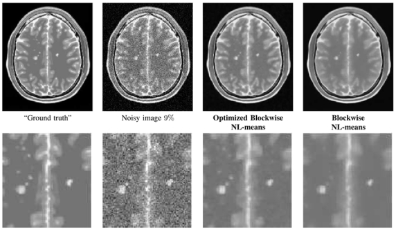
NL-means restoration of T2-w Brainweb data with MS lesions. From left to right: “Ground truth”, noised image at 9% of Gaussian noise, restored images by the Optimized Blockwise NL-means filter and by the Blockwise NL-means filter. The Optimized Blockwise NL-means filter preserves efficiently the contours of the MS lesions.

G. Comparison with other denoising methods

1. Focus on two classical denoising approaches

a. Anisotropic Diffusion filtering

As reported in Section II, the Anisotropic Diffusion filter (AD) was introduced to overcome the blurring effect of the Gaussian smoothing approach. First introduced by Perona and Malik [3], in this approach the image u is only convolved in the direction orthogonal to the gradient of the image which ensures the preservation of edges. The iterative denoising process of initial image u₀ can be expressed as:

$$\{\begin{array}{l}\frac{\partial u(x,t)}{\partial t}=\text{div}(c(x,t)\nabla u(x,t))\hfill \\ u(x,0)=u_0(x)\hfill \end{array}$$ (14)

where ∇ u(x, t) is the image gradient at voxel x and iteration t, $\frac{\partial u(x,t)}{\partial t}$ is the partial temporal deviation of u(x, t) and

$$c(x,t)=g(\parallel \nabla u(x,t)\parallel )=e^{-\frac{\parallel \nabla u(x,t)\parallel }{K^2}}$$ (15)

where K is the diffusivity parameter. The AD filter method produces a good preservation of edges [34], [35]. Nonetheless, the main disadvantage of Ad filter is to poorly denoise the constant regions (see Fig. 13).

Fig. 13. Comparison with Anisotropic Diffusion, Total Variation and NL-means denoising on synthetic T1-w images.

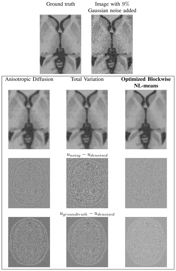
Top: zooms on T1-w BrainWeb images. Left: the “ground truth”. Right: the noisy images with 9% of Gaussian noise. Middle: the results of restoration obtained with the different methods and the images of the removed noise (i.e. the difference (centered on 128) between the noisy image and the denoised image. Bottom: the difference (centered on 128) between the denoised image and the ground truth. Left: Anisotropic Diffusion denoising. Left: Anisotropic Diffusion denoising. Middle: Total Variation minimization process. Right: Optimized Blockwise NL-means filter. The NL-means based restoration better preserves the anatomical structure in the image while efficiently removing the noise as it can be seen in the image of removed noise.

b. Total Variation minimization scheme

The difficult task to preserve edges while correctly denoising constant areas has been addressed also by Rudin, Osher and Fatemi. They proposed to minimize the Total Variation (TV) norm subject to noise constraints [4], that is:

$$\widehat{u}=arg\underset{u\in {\mathrm{\Omega }}^3}{min}\int \mid \nabla u(x)\mid dx$$ (16)

subject to

$${\int }_{{\mathrm{\Omega }}^3}(u(x)-u_0(x))dx=0\text{and}{\int }_{{\mathrm{\Omega }}^3}\mid u(x)-u_0(x){\mid }^{2}dx={\sigma }^2$$ (17)

where u₀ is the original noisy image, u is the restored image and σ the standard deviation of the noise. In this model, the TV minimization tends to smooth inside the image structures while keeping the integrity of boundaries. The TV minimization scheme can be expressed as an unconstrained problem:

$$\widehat{u}=arg\underset{u\in {\mathrm{\Omega }}^3}{min}\left[{\int }_{{\mathrm{\Omega }}^3}\mid \nabla u(x)\mid dx+\lambda {\int }_{{\mathrm{\Omega }}^3}\mid u(x)-u_0(x){\mid }^{2}dx\right]$$ (18)

where λ is a Lagrange multiplier which controls the balance between the TV norm and the fidelity term. Thus, λ acts as the filtering parameter. Indeed, for high values for λ the fidelity term is encouraged. For small values for λ the regularity term is desired. In practice, the TV minimization scheme tends to remove texture and small image structures as seen in Fig. 13 [36]. To solve this problem, iterative total variation schemes have been recently developed [55], [56].

2. Quantitative and qualitative comparison

The main difficulty to achieve this comparison is related to the tuning of smoothing parameters in order to obtain the best results for AD filter and TV minimization scheme. In order not to penalize AD filter and TV minimization scheme, an exhaustive search for all parameters into a certain range. Then, the best results obtained with AD filter and TV minimization have been selected, whereas the fully-automatic results have been mentioned for the NL-means filters. The results of the NL-means filters are not “optimal” due to the non perfect estimation of the noise standard deviation. For AD filter, the parameter K varies from 0.05 to 1 with a step of 0.05 and the number of iterations varies from 1 to 10. For TV minimization, the parameter λ varies from 0.01 to 1 with step of 0.01 and the number of iterations varies from 1 to 10. The results obtained for 9% of Gaussian noise are presented Fig. 11, but this screening have been performed for the four levels of noise. It is important to underline that the results giving the best PSNR are used, but these results do not necessary give the best visual output. Indeed, the best PSNR for AD filter is obtained for a visually under-smoothed image since this method tends to spoil the edges. To obtain a high PSNR, the denoised image needs to balance edge preserving and noise removing. For AD filter, this trade-off leads to inhomogeneities in flat areas in denoised image (see Fig. 13). For TV minimization, the best PSNR is obtained with a visually under-smoothed image since noise is present in denoised image (see Fig. 13).

Fig. 11.

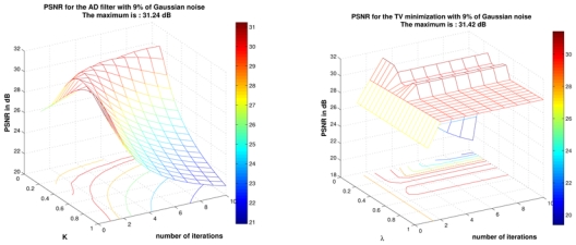
Result for AD filter and TV minimization on phantom images with Gaussian noise at 9%. For AD filter K varies from 0.05 to 1 with step of 0.05 and the number of iterations varies from 1 to 10. For TV minimization λ varies from 0.01 to 1 with step of 0.01 and the number of iterations varies from 1 to 10

a. PSNR comparison

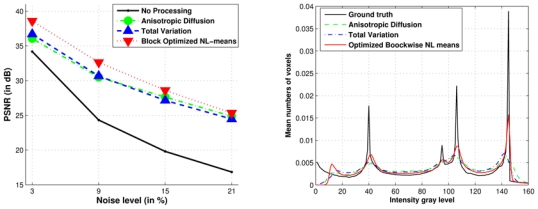
As presented in Fig. 12 (left), our block optimized NL-means filter produces the best PSNR values whatever the noise level. On average, a gain of 1.85 dB is measured compared to TV and Anisotropic Diffusion methods. The PSNR value between the noisy image and the ground truth is called “No processing” and is used as reference.

Fig. 12. Comparison between Anisotropic Diffusion, Total Variation and Optimized Blockwise NL-means denoising.

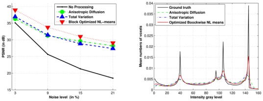
the PSNR values and histograms for different denoising methods on BrainWeb at 9% of Gaussian noise. Left: the PSNR experiment shows that the Optimized Blockwise NL-means filter outperforms the well-established Total Variation minimization process and the Anisotropic Diffusion approach. Right: Contrary to others methods, the NL-means based restoration clearly distinguishes the three main peaks representing the white matter, the gray matter and the cerebrospinal fluid. The sharpness of the peaks shows how the Optimized Blockwise NL-means filter increases the contrast between denoised biological structures.

b. Histogram comparison

To better understand how these differences in the PSNR values between the three methods can be explained, the histograms of the denoised images were compared to the histogram of the ground truth. Figure 12 (right) shows that the Optimized Blockwise NL-means filter is the only method able to retrieve a histogram similar to the ground truth. The NL-means-based restoration schemes clearly distinguish the three main peaks representing the white matter, the gray matter and the cerebrospinal fluid. The sharpness of the peaks shows how the Optimized Blockwise NL-means filter increases the contrast between denoised biological structures (see also Fig. 13). The distances between these histograms are estimated with the Bhattacharyya coefficient (BC) defined as:

$$BC(p,q)=\sum _{b=0}^{255}\sqrt{p(b)q(b)}$$ (19)

where p and q are the two histograms be to compared and b is the bin index. A BC close to 1 means p and q are very similar. Each histogram of denoised images is compared to the “ground truth” one (see Tab. III). The distance between the histogram of the noisy image and the histogram of the “ground truth” is used as a reference. The BC distance shows that the restored histogram obtained with the Optimized Blockwise NL-means filter is the closest to the “ground truth”, as visually assessed in Figure 12 (right). Finally, Table III suggests that the NL-means-based approach could improve the registration of images, since the Mutual Information (MI) computed between the restored image and the “ground truth” is higher in comparison with AD filter and TV minimization. The MI is a similarity measure commonly used in image registration.

TABLE III. Comparison of histograms obtained with the three different methods at 9% of Gaussian noise.

This Table presents (a) the Bhattacharyya coefficient computed between the histograms of denoised images and the “ground truth” one and (b) the mutual information computed between the denoised images and the “ground truth” The distance between the noisy image and the “ground truth” is used as a reference. Compared to AD filter and TV minimization, the Optimized Blockwise NL-means filter allows to obtain a denoised image whose histogram is more closer to “ground truth” histogram.

	Bhattacharyya Coefficient	Mutual Information
Noisy image	0.9388	1.282
Anisotropic diffusion	0.9608	2.024
Total Variation	0.9639	1.974
Optimized Blockwise NL-means	0.9756	2.214

c. Visual Assessment

Figures 13 and 14 show the restored images and the removed noise obtained with the three compared methods. As shown in the previous analysis, we observe that the homogeneity of white matter is higher when the image is denoised with the Optimized Blockwise NL-means filter. Moreover, focusing on the structure of the removed noise, it clearly appears that NL-means-based restoration schemes better preserves the high frequency components of the image corresponding to anatomical structures while removing efficiently the high frequencies due to noise. According to the “method noise” introduced in [57], the NL-means is a better denoising method since the removed noise is the most similar to a white Gaussian noise. Finally, the difference between the “ground truth” and the denoised image is presented in order to show which structures are removed during the denoising process. In Fig. 13, this difference shows that (a) the AD filter tends to spoil the edges especially on the skull, (b) the TV minimization slightly better preserves the edges but does not remove all the noise, and (c) the Optimized Blockwise NL-means filter visually better preserves the edges while efficiently removing the noise (especially for white matter).

Fig. 14. Comparison with Anisotropic Diffusion, Total Variation and NL-means denoising on synthetic T1-w images.

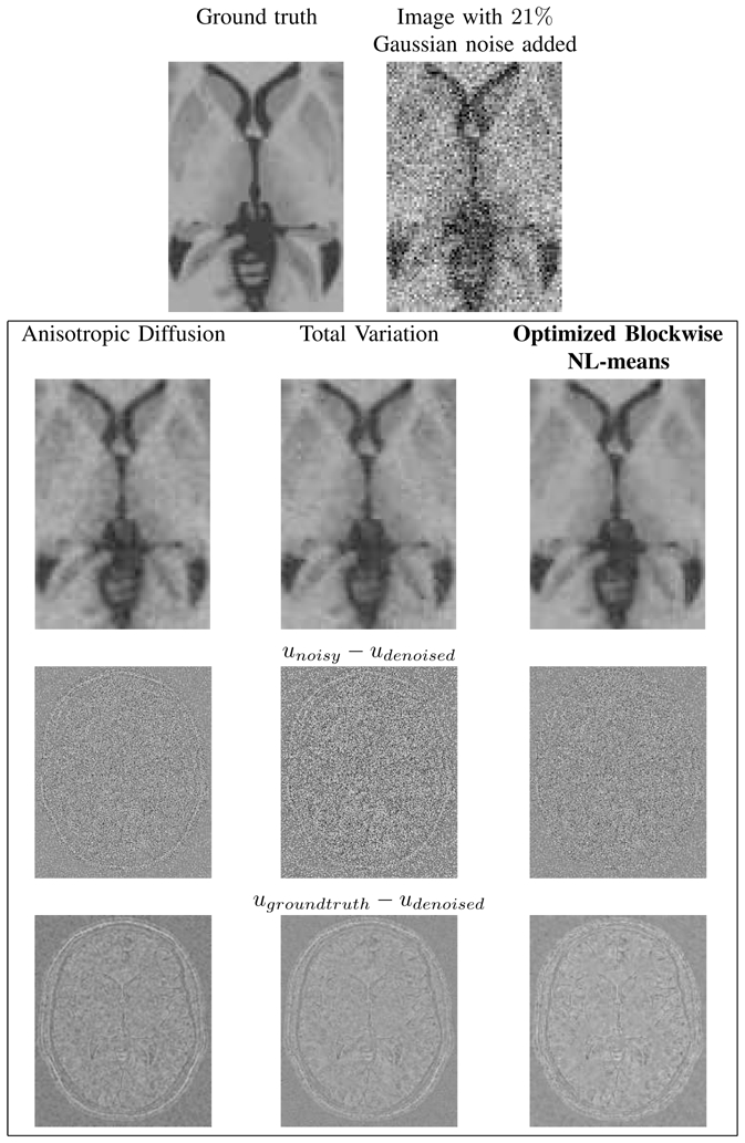
Top: zooms on T1-w BrainWeb images. Left: the “ground truth”. Right: the noisy images with 21% of Gaussian noise. Middle: the results of restoration obtained with the different methods and the images of the removed noise (i.e. the difference (centered on 128) between the noisy image and the denoised image. Bottom: the difference (centered on 128) between the denoised image and the ground truth. Left: Anisotropic Diffusion denoising. Middle: Total Variation minimization process. Right: Optimized Blockwise NL-means filter.

VI. Validation on a Phantom data set with added Rician Noise

In this section, the same experiments are performed on phantom data set corrupted by Rician noise in order to study the impact of the Gaussian assumption. Table IV shows the computation time and the denoising performance of the different compared NL-means filters. These results show that the optimized NL-means versions outperform the classical ones also for Rician noise. Figure 15 presents the comparison with AD filter and TV minimization in terms of PSNR values and histogram analysis. As for the AD filter and TV minimization, the NL-means-based denoising is able to correctly restore an image corrupted by Rician noise using a Gaussian approximation. When the histograms are compared, low values of intensity (< 20) are incorrectly restored for all the filters; the Gaussian approximation is not appropriate in that case. Nevertheless, it seems the underlying assumption is well suited to high values (> 60).

TABLE IV. Comparison of different implementations of the NL-means filter in terms of computational time and denoising quality.

These results are obtained on a T1-w BrainWeb image with 9% of Rician noise on a Intel(R) Pentium(R) D CPU 3.40GHz with 2Go of RAM. The parameters used are the default parameters. The average number of voxels/blocks used in V_i to denoise x_i shows the impact of voxels/blocks selection. For non-optimized implementations all the voxels/blocks in V_i are taken into account to denoise x_i. Thus, the number of voxels/blocks used are |V_i| = (2M + 1)³ = 11³. For optimized implementations the voxel selection allows to drastically reduce this number.

Rician Noise	Computational time (in s)	PSNR (in dB)	Average number of voxels/blocks used in Vi to denoise xi
NL-means	4190	31.35	113 = 1331 voxels
Blockwise NL-means	759	30.90	113 = 1331 blocks
Optimized NL-means	1045	33.40	251.1 voxels
Optimized Blockwise NL-means	169	32.64	251.1 blocks

Fig. 15. Comparison with Anisotropic Diffusion, Total Variation and Optimized Blockwise NL-means denoising.

PSNR values and histograms for different denoising methods on BrainWeb at 9% of Rician noise. Left: the PSNR study shows that the Optimized Blockwise NL-means filter outperforms the well-established Total Variation minimization process and the Anisotropic Diffusion approach. Right: When the histograms are compared low values of intensity (< 20) are incorrectly restored for all the filters; the Gaussian approximation is not appropriate in that case. Nevertheless, it seems the underlying assumption is well suited to high values (> 60). Contrary to others methods, the NL-means based restoration clearly emphasizes the three main peaks representing the white matter, the gray matter and the cerebrospinal fluid. The sharpness of the peaks shows how the Optimized Blockwise NL-means filter increases the contrast between denoised biological structures.

As for Gaussian noise, the NL-means-based restoration clearly emphasizes the three main peaks corresponding to the white matter, the gray matter and the cerebrospinal fluid. Figure 16 shows the visual results obtained when the methods are compared on phantom data with Rician noise. Compared to Fig. 13, the denoising of background is worse in the Rician case, but the cerebral structures are correctly restored with the NL-means filter especially the white matter (see Fig. 16). Finally, Figure 17 shows the PSNR results of the parameter screening for the AD filter and the TV minimization at 9% of Rician noise. All these results on Rician noise show that the PNSR values slightly decrease due to more pronounced noise compared to Gaussian case for a same level (see IV-A.2 for explanation), but the general performance of the filters is preserved.

Fig. 16. Comparison with Anisotropic Diffusion, Total Variation and NL-means denoising on synthetic T1-w images.

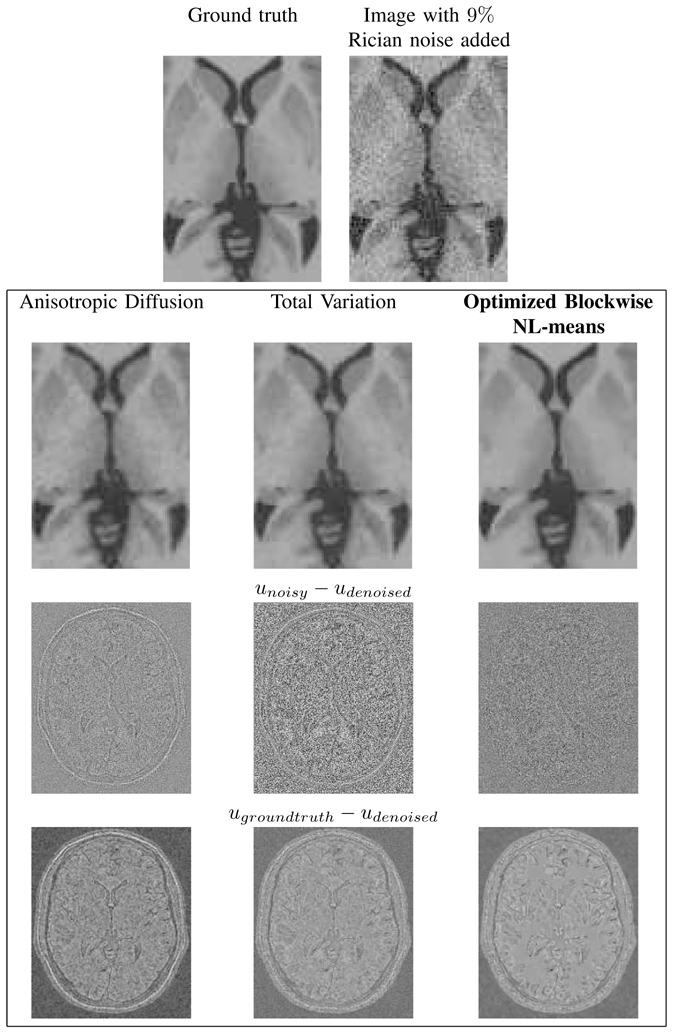
Top: zooms on T1-w BrainWeb images. Left: the “ground truth”. Right: the noisy images with 9% of Rician noise. Middle: the results of restoration obtained with the different methods and the images of the removed noise (i.e. the difference (centered on 128) between the noisy image and the denoised image. Bottom: the “Method Noise” which is the difference (centered on 128) between the denoised image and the ground truth. Left: Anisotropic Diffusion denoising. Middle: Total Variation minimization process. Right: Optimized Blockwise NL-means filter. The NL-means based restoration better preserves the anatomical structure in the image while efficiently removing the noise, it can be seen in the image of removed noise.

Fig. 17.

Result for AD filter and TV minimization on phantom images with 9% of Rician noise. For AD filter K varies from 0.05 to 1 with step of 0.05 and the number of iterations varies from 1 to 10. For TV minimization λ varies from 0.01 to 1 with step of 0.01 and the number of iterations varies from 1 to 10.

VII. Experiments on clinical data

A. High field MRI

The restoration results presented in Fig. 18 show good preservation of the cerebellum contours. Fully automatic segmentation and quantitative analysis of such structures are still a challenge, and improved restoration schemes could greatly improve these processings.

Fig. 18. NL-means filter on a real T1-w MRI.

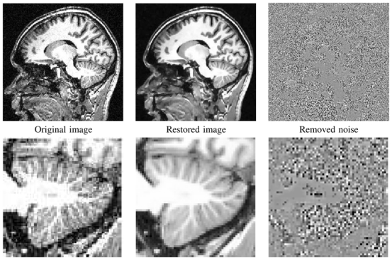
Fully-automatic restoration obtained with the Optimized Blockwise NL-means filter on a 3 Tesla T1-w MRI data of 256³ voxels in less than 3 minutes on a Intel(R) Pentium(R) D CPU 3.40GHz with 2Go of RAM. From left to right: Original image, denoised image, and difference image with gray values centered on 128. The whole image is shown on top, and a detail is displayed on bottom.

B. MS pathological context

Figure 19 shows that the optimized blockwise NL-means filter preserves the lesions while removing the noise. The impact on further processing is not the scope of this paper and is not studied here. Nevertheless, visually the lesions appears more contrasted and as seen on the difference image the proposed NL-means approach does not include any structure of lesion in the estimated noise image. This was confirmed by an experienced neurologist.

Fig. 19. NL-means filter on a real T2-w MRI with MS.

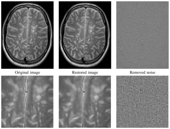
Fully-automatic restoration obtained with the Optimized Blockwise NL-means filter on a 1.5T T2-w MRI data with MS lesions of 512 × 512 × 28 voxels in less than 2 minute on a Intel(R) Pentium(R) D CPU 3.40GHz with 2Go of RAM. From left to right: Original image, denoised image, and difference image with gray values centered on 128. The whole image is shown on top, and a detail is exposed on bottom.

VIII. Discussion and Conclusion

This paper presents an optimized blockwise version of the Non Local (NL-) means filter, applied to 3D medical data. Validation was performed on the BrainWeb dataset [2] and showed that the proposed Optimized Blockwise NL-means filter outperforms the classical implementation of the NL-means filter and some state-of-the-art techniques, such as the Anisotropic Diffusion approach [3] and the Total Variation minimization process [4] on both Gaussian and Rician noise. These first results show that the image-redundancy assumption required for NL-means based restoration holds for 3D MRI. Compared to the classical NL-means filter, our implementation (with voxel preselection, multithreading and blockwise implementation) considerably decreases the required computational time (up to a factor of 60 on a Xeon at 3GHz) and increases the PSNR value of the denoised image. Nevertheless, the problem of the computational burden can still be investigated with other faster implementations such as the “plain multiscale” scheme also suggested in [1]. Further works should be pursued for comparing NL-means based restoration with recent promising denoising methods, such as Total Variation in wavelet domain [43] or adaptive estimation method [28], [50]. Moreover, the efficiency of the technique limiting the staircasing effect proposed in [58] needs to be studied for MRI.

We show on sample pathological cases (patients with MS lesions) that the filter preserves the major visual signature of the given pathology. However, the impact on specific pathologies needs to be further investigated.

Finally, the impact of the NL-means-based denoising on the performances of post-processing algorithms, like segmentation and registration schemes also should be studied. Nonetheless, the first results presented on the Mutual Information (MI) suggest that the proposed Optimized Blockwise NL-means filter could improve the image registration process. Indeed, the MI computed between the restored image and the “ground truth” is higher with the Optimized Blockwise NL-means filter than with the Anisotropic Diffusion approach and the Total Variation minimization process.

TABLE I. Peak Signal to Noise Ratio (PSNR) between “Ground Truth” and noisy images for Gaussian and Rician noises.

For a same level of noise, the Rician noise is stronger than the Gaussian noise.

Noise level	PSNR with Gaussian noise in dB	PSNR with Rician noise in dB
3%	35.09	35.05
9%	25.64	25.57
15%	21.30	21.17
21%	18.49	18.29

References

- 1.Buades A, Coll B, Morel JM. A review of image denoising algorithms, with a new one. Multiscale Modeling & Simulation. 2005;4(2):490–530. [Google Scholar]
- 2.Collins D, Zijdenbos A, Kollokian V, Sled J, Kabani N, Holmes C, Evans A. Design and construction of a realistic digital brain phantom. IEEE Trans Med Imaging. 1998;17(3):463–468. doi: 10.1109/42.712135. [DOI] [PubMed] [Google Scholar]
- 3.Perona P, Malik J. Scale-space and edge detection using anisotropic diffusion. IEEE Trans Pattern Anal Mach Intell. 1990;12(7):629–639. [Google Scholar]
- 4.Rudin L, Osher S, Fatemi E. Nonlinear total variation based noise removal algorithms. Physica D. 1992;60:259–268. [Google Scholar]
- 5.Mazziotta J, Toga A, Evans A, Fox P, Lancaster J, Zilles K, Woods R, Paus T, Simpson G, Pike B, Holmes C, Collins L, Thompson P, MacDonald D, Iacoboni M, Schormann T, Amunts K, Palomero-Gallagher N, Geyer S, Parsons L, Narr K, Kabani N, Le Goualher G, Boomsma D, Cannon T, Kawashima R, Mazoyer B. A probabilistic atlas and reference system for the human brain: International consortium for brain mapping (icbm) Philos Trans R Soc Lond B Biol Sci. 2001 Aug;356(1412):1293–1322. doi: 10.1098/rstb.2001.0915. [DOI] [PMC free article] [PubMed] [Google Scholar]
- 6.Zijdenbos A, Forghani R, Evans A. Automatic” pipeline” analysis of 3D MRI data for clinical trials: application to multiple sclerosis. IEEE Trans Med Imaging. 2002 Oct;21(10):1280–1291. doi: 10.1109/TMI.2002.806283. [DOI] [PubMed] [Google Scholar]
- 7.Geman S, Geman D. Stochastic relaxation, Gibbs distribution, and the Bayesian restoration of images. IEEE Trans PAMI. 1984;6:721–741. doi: 10.1109/tpami.1984.4767596. [DOI] [PubMed] [Google Scholar]
- 8.Mumford SJD. Optimal approximations by piecewise smooth functions and variational problems. Comm Pure and Appl Math. 1989;42:577–685. [Google Scholar]
- 9.Tschumperlé D. ECCV. Graz: 2006. Curvature-preserving regularization of multi-valued images using PDE’s; pp. 428–433. [Google Scholar]
- 10.Black M, Sapiro G. Edges as outliers: Anisotropic smoothing using local image statistics. Scale-Space Theories in Computer Vision, Second International Conference, Scale-Space ‘99, Proceedings; Corfu, Greece. September 26–27, 1999; 1999. pp. 259–270. [Google Scholar]
- 11.Saint-Marc P, Chen JS, Medioni G. Adaptive smoothing: a general tool for early vision. IEEE Transactions on Pattern Analysis and Machine Intelligence. 1991 Jun;13(6):514–529. [Google Scholar]
- 12.Donoho D, Johnstone I. Ideal spatial adaptation by wavelet shrinkage. Biometrika. 1994;81(3):425–455. [Google Scholar]
- 13.Donoho D. De-noising by soft-thresholding. IEEE Transactions on Information Theory. 1995;41(3):613–627. [Google Scholar]
- 14.Portilla J, Simoncelli E. Image restoration using Gaussian scale mixtures in the wavelet domain. ICIP ‘03: International Conference on Image Processing; 2003. pp. 965–968. [Google Scholar]
- 15.Tomasi C, Manduchi R. Bilateral filtering for gray and color images. ICCV ‘98: Proceedings of the Sixth International Conference on Computer Vision; Washington, DC, USA: IEEE Computer Society; 1998. p. 839. [Google Scholar]
- 16.Smith S, Brady J. SUSAN–A New Approach to Low Level Image Processing. International Journal of Computer Vision. 1997 May;23(1):45–78. [Google Scholar]
- 17.Elad M. On the origin of the bilateral filter and ways to improve it. IEEE Transactions on Image Processing. 2002 Oct;11(10):1141–1151. doi: 10.1109/TIP.2002.801126. [DOI] [PubMed] [Google Scholar]
- 18.van de Weije J, van den Boomgaard R. Local mode filtering. CVPR ‘01: IEEE Computer Society Conference on Computer Vision and Pattern Recognition; 8–14 December; Kauai, HI, USA. 2001. pp. 428–433. [Google Scholar]
- 19.Chan T, Zhou H. Total variation improved wavelet thresholding in image compression. ICIP; 2000. [Google Scholar]
- 20.Durand S, Froment J. Reconstruction of wavelet coefficients using total variation minimization. SIAM J Sci Comput. 2002;24(5):1754–1767. [Google Scholar]
- 21.Lintner S, Malgouyres F. Solving a variational image restoration model which involves L∞ constraints. Inverse Problems. 2004;20(3):815–831. [Google Scholar]
- 22.Mrazek P, Weickert J, Bruhn A. On robust estimation and smoothing with spatial and tonal kernels. Preprint. 2004;51 [Google Scholar]
- 23.Barash D. A fundamental relationship between bilateral filtering, adaptive smoothing, and the nonlinear diffusion equation. IEEE Trans Pattern Anal Mach Intell. 2002 Jun;24(6):844–847. [Google Scholar]
- 24.Sapiro G. From active contours to anisotropic diffusion: connections between basic PDE’s in image processing. ICIP ‘96: International Conference on Image Processing; 1996. pp. 477–480. [Google Scholar]
- 25.Polzehl SVJ. Adaptive weights smoothing with application to image restoration. J Roy Stat Soc B. 2000;62:335–354. [Google Scholar]
- 26.Katkovnik V, Egiazarian K, Astola J. Adaptive window size image de-noising based on intersection of confidence intervals (ICI) rule. J Math Imaging Vis. 2002 May;16(3):223–235. [Google Scholar]
- 27.Kervrann C. An adaptive window approach for image smoothing and structures preserving. Computer Vision - ECCV 2004, 8th European Conference on Computer Vision, Proceedings, Part III; Prague, Czech Republic. May 11–14, 2004; 2004. pp. 132–144. [Google Scholar]
- 28.Kervrann C, Boulanger J. Unsupervised patch-based image regularization and representation. Proc. European Conf. Comp. Vision (ECCV ‘06); Graz, Austria. May 2006.. [Google Scholar]
- 29.Kervrann C, Boulanger J. Optimal spatial adaptation for patch-based image denoising. IEEE Trans. on Image Processing; 2006. [DOI] [PubMed] [Google Scholar]
- 30.Zhu S, Wu Y, Mumford D. Filters, random fields and maximum entropy (frame): Towards a unified theory for texture modeling. Int J Comput Vision. 1998;27(2):107–126. [Google Scholar]
- 31.Freeman W, Pasztor E, Carmichael O. Learning low-level vision. Int J Comput Vision. 2000 Oct;40(1):25–47. [Google Scholar]
- 32.Roth S, Black M. Fields of experts: A framework for learning image priors. 2005 IEEE Computer Society Conference on Computer Vision and Pattern Recognition (CVPR 2005); 20–26 June 2005; San Diego, CA, USA. 2005. pp. 860–867. [Google Scholar]
- 33.Awate S, Whitaker R. Higher-order image statistics for unsupervised, information-theoretic, adaptive, image filtering. IEEE Computer Society Conference on Computer Vision and Pattern Recognition (CVPR 2005); San Diego, CA, USA: IEEE Computer Society; Jun, 2005. pp. 44–51. [Google Scholar]
- 34.Gerig G, Kikinis R, Kübler O, Jolesz F. Nonlinear anisotropic filtering of MRI data. IEEE Transactions on Medical Imaging. 1992 Jun;11(2):221–232. doi: 10.1109/42.141646. [DOI] [PubMed] [Google Scholar]
- 35.Weickert J, ter Haar Romeny BM, Viergever MA. Efficient and reliable schemes for nonlinear diffusion filtering. IEEE Transactions on Image Processing. 1998;7(3):398–410. doi: 10.1109/83.661190. [DOI] [PubMed] [Google Scholar]
- 36.Keeling S. Total variation based convex filters for medical imaging. Appl Math Comput. 2003;139(1):101–119. [Google Scholar]
- 37.Wong W, Chung A, Yu S. Trilateral filtering for biomedical images. IEEE International Symposium on Biomedical Imaging: From Nano to Macro; Arlington, VA, USA. 15–18 April 2004; 2004. pp. 820–823. [Google Scholar]
- 38.Nowak R. Wavelet-based Rician noise removal for magnetic resonance imaging. IEEE Transactions on Image Processing. 1999 Oct;8(10):1408–1419. doi: 10.1109/83.791966. [DOI] [PubMed] [Google Scholar]
- 39.Wood J, Johnson K. Wavelet packet denoising of magnetic resonance images: importance of Rician noise at low SNR. Magn Reson Med. 1999 Mar;41(3):631–635. doi: 10.1002/(sici)1522-2594(199903)41:3<631::aid-mrm29>3.0.co;2-q. [DOI] [PubMed] [Google Scholar]
- 40.Zaroubi S, Goelman G. Complex denoising of MR data via wavelet analysis: application for functional MRI. Magn Reson Imaging. 2000 Jan;18(1):59–68. doi: 10.1016/s0730-725x(99)00100-9. [DOI] [PubMed] [Google Scholar]
- 41.Alexander ME, Baumgartner R, Summers AR, Windischberger C, Klarhoefer M, Moser E, Somorjai RL. A wavelet-based method for improving signal-to-noise ratio and contrast in MR images. Magn Reson Imaging. 2000 Feb;18(2):169–180. doi: 10.1016/s0730-725x(99)00128-9. [DOI] [PubMed] [Google Scholar]
- 42.Bao P, Zhang L. Noise reduction for magnetic resonance images via adaptive multiscale products thresholding. IEEE Trans Med Imaging. 2003 Sep;22(9):1089–1099. doi: 10.1109/TMI.2003.816958. [DOI] [PubMed] [Google Scholar]
- 43.Ogier A, Hellier P, Barillot C. Restoration of 3D medical images with total variation scheme on wavelet domains (TVW). Proceedings of SPIE Medical Imaging 2006: Image Processing; San Diego, USA. February 2006.. [Google Scholar]
- 44.Wang Y, Zhou H. Total variation wavelet-based medical image denoising. International Journal of Biomedical Imaging. 2006;2006:6. doi: 10.1155/IJBI/2006/89095. Article ID 89 095. [DOI] [PMC free article] [PubMed] [Google Scholar]
- 45.McDonnell M. Box-filtering techniques. Computer Vision, Graphics, and Image Processing. 1981 Sep;17(1):65–70. [Google Scholar]
- 46.Yaroslavsky L. In: Digital Picture Processing - An Introduction. Verlag S, editor. 1985. [Google Scholar]
- 47.Lee J. Digital image smoothing and the sigma filter. Computer Vision, Graphics and Image Processing. 1983;24:255–269. [Google Scholar]
- 48.Coifman R, Donoho D. Lecture Notes in Statistics: Wavelets and Statistics. New York: Feb, 1995. Translation invariant de-noising; pp. 125–150. [Google Scholar]
- 49.Gasser T, Sroka L, Steinmetz C. Residual variance and residual pattern in nonlinear regression. Biometrika. 1986;73(3):625–633. [Google Scholar]
- 50.Boulanger J, Kervrann C, Bouthemy P. Adaptive spatio-temporal restoration for 4D fluoresence microscopic imaging. Int. Conf. on Medical Image Computing and Computer Assisted Intervention (MICCAI’ 05); Palm Springs, USA. October 2005.; [DOI] [PubMed] [Google Scholar]
- 51.Buades A, Coll B, Morel J-M. Image and movie denoising by nonlocal means. CMLA, Tech Rep. 2006;25 [Google Scholar]
- 52.Mahmoudi M, Sapiro G. Fast image and video denoising via nonlocal means of similar neighborhoods. Signal Processing Letters, IEEE. 2005;12(12):839–842. [Google Scholar]
- 53.Gudbjartsson H, Patz S. The Rician distribution of noisy MRI data. Magnetic Resonance in Medicine. 1995;34:910–914. doi: 10.1002/mrm.1910340618. [DOI] [PMC free article] [PubMed] [Google Scholar]
- 54.Macovski A. Noise in MRI. Magnetic Resonance in Medicine. 1996;36:494–497. doi: 10.1002/mrm.1910360327. [DOI] [PubMed] [Google Scholar]
- 55.Osher S, Burger M, Goldfarb D, Xu J, Yin W. An iterative regularization method for total variation-based image restoration. Multiscale Model Simul. 2005;4(2):460–489. [Google Scholar]
- 56.Tadmor E, Nezzar S, Vese L. A multiscale image representation using hierarchical (BV, L2) decompositions. Multiscale Model Simul. 2004;2(4):554–579. [Google Scholar]
- 57.Buades A, Coll B, Morel J-M. A non local algorithm for image denoising. San Diego, USA: IEEE Computer Society; Jun, 2005. pp. 60–65. [Google Scholar]
- 58.Buades A, Coll B, Morel JM. The staircasing effect in neighborhood filters and its solution. IEEE Transactions on Image Processing. 2006;15(6):1499–1505. doi: 10.1109/tip.2006.871137. [DOI] [PubMed] [Google Scholar]