Bayesian inference for generalized linear mixed models

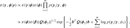
Abstract

Generalized linear mixed models (GLMMs) continue to grow in popularity due to their ability to directly acknowledge multiple levels of dependency and model different data types. For small sample sizes especially, likelihood-based inference can be unreliable with variance components being particularly difficult to estimate. A Bayesian approach is appealing but has been hampered by the lack of a fast implementation, and the difficulty in specifying prior distributions with variance components again being particularly problematic. Here, we briefly review previous approaches to computation in Bayesian implementations of GLMMs and illustrate in detail, the use of integrated nested Laplace approximations in this context. We consider a number of examples, carefully specifying prior distributions on meaningful quantities in each case. The examples cover a wide range of data types including those requiring smoothing over time and a relatively complicated spline model for which we examine our prior specification in terms of the implied degrees of freedom. We conclude that Bayesian inference is now practically feasible for GLMMs and provides an attractive alternative to likelihood-based approaches such as penalized quasi-likelihood. As with likelihood-based approaches, great care is required in the analysis of clustered binary data since approximation strategies may be less accurate for such data.

1. INTRODUCTION

Generalized linear mixed models (GLMMs) combine a generalized linear model with normal random effects on the linear predictor scale, to give a rich family of models that have been used in a wide variety of applications (see, e.g. Diggle and others, 2002, Verbeke and Molenberghs, 2000, Verbeke and Molenberghs, 2005, McCulloch and others, 2008). This flexibility comes at a price, however, in terms of analytical tractability, which has a number of implications including computational complexity, and an unknown degree to which inference is dependent on modeling assumptions. Likelihood-based inference may be carried out relatively easily within many software platforms (except perhaps for binary responses), but inference is dependent on asymptotic sampling distributions of estimators, with few guidelines available as to when such theory will produce accurate inference. A Bayesian approach is attractive, but requires the specification of prior distributions which is not straightforward, in particular for variance components. Computation is also an issue since the usual implementation is via Markov chain Monte Carlo (MCMC), which carries a large computational overhead. The seminal article of Breslow and Clayton (1993) helped to popularize GLMMs and placed an emphasis on likelihood-based inference via penalized quasi-likelihood (PQL). It is the aim of this article to describe, through a series of examples (including all of those considered in Breslow and Clayton, 1993), how Bayesian inference may be performed with computation via a fast implementation and with guidance on prior specification.

The structure of this article is as follows. In Section 2, we define notation for the GLMM, and in Section 3, we describe the integrated nested Laplace approximation (INLA) that has recently been proposed as a computationally convenient alternative to MCMC. Section 4 gives a number of prescriptions for prior specification. Three examples are considered in Section 5 (with additional examples being reported in the supplementary material available at Biostatistics online, along with a simulation study that reports the performance of INLA in the binary response situation). We conclude the paper with a discussion in Section 6.

2. THE GENERALIZED LINEAR MIXED MODEL

GLMMs extend the generalized linear model, as proposed by Nelder and Wedderburn (1972) and comprehensively described in McCullagh and Nelder (1989), by adding normally distributed random effects on the linear predictor scale. Suppose Y_ij is of exponential family form: Y_ij|θ_ij,ϕ₁ ∼ p(·), where p(·) is a member of the exponential family, that is,

for i = 1,…,m units (clusters) and j = 1,…,n_i, measurements per unit and where θ_ij is the (scalar) canonical parameter. Let μ_ij = E[Y_ij|β,b_i,ϕ₁] = b^′(θ_ij) with

where g(·) is a monotonic “link” function, x_ij is 1 × p, and z_ij is 1 × q, with β a p × 1 vector of fixed effects and b_i a q × 1 vector of random effects, hence θ_ij = θ_ij(β,b_i). Assume b_i|Q ∼ N(0,Q ^{− 1}), where the precision matrix Q = Q(ϕ₂) depends on parameters ϕ₂. For some choices of model, the matrix Q is singular; examples include random walk models (as considered in Section 5.2) and intrinsic conditional autoregressive models. We further assume that β is assigned a normal prior distribution. Let γ = (β,b) denote the G × 1 vector of parameters assigned Gaussian priors. We also require priors for ϕ₁ (if not a constant) and for ϕ₂. Let ϕ = (ϕ₁,ϕ₂) be the variance components for which non-Gaussian priors are assigned, with V = dim(ϕ).

3. INTEGRATED NESTED LAPLACE APPROXIMATION

Before the MCMC revolution, there were few examples of the applications of Bayesian GLMMs since, outside of the linear mixed model, the models are analytically intractable. Kass and Steffey (1989) describe the use of Laplace approximations in Bayesian hierarchical models, while Skene and Wakefield (1990) used numerical integration in the context of a binary GLMM. The use of MCMC for GLMMs is particularly appealing since the conditional independencies of the model may be exploited when the required conditional distributions are calculated. Zeger and Karim (1991) described approximate Gibbs sampling for GLMMs, with nonstandard conditional distributions being approximated by normal distributions. More general Metropolis–Hastings algorithms are straightforward to construct (see, e.g. Clayton, 1996, Gamerman, 1997). The winBUGS (Spiegelhalter, Thomas, and Best, 1998) software example manuals contain many GLMM examples. There are now a variety of additional software platforms for fitting GLMMs via MCMC including JAGS (Plummer, 2009) and BayesX (Fahrmeir and others, 2004). A large practical impediment to data analysis using MCMC is the large computational burden. For this reason, we now briefly review the INLA computational approach upon which we concentrate. The method combines Laplace approximations and numerical integration in a very efficient manner (see Rue and others, 2009, for a more extensive treatment). For the GLMM described in Section 2, the posterior is given by

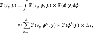
where y_i = (y_i1,…,y_ini) is the vector of observations on unit/cluster i. We wish to obtain the posterior marginals π(γ_g|y), g = 1,…,G, and π(ϕ_v|y), v = 1,…,V. The number of variance components, V, should not be too large for accurate inference (since these components are integrated out via Cartesian product numerical integration, which does not scale well with dimension). We write

which may be evaluated via the approximation

(3.1)

where Laplace (or other related analytical approximations) are applied to carry out the integrations required for evaluation of . To produce the grid of points {ϕ^k,k = 1,…,K} over which numerical integration is performed, the mode of is located, and the Hessian is approximated, from which the grid is created and exploited in (3.1). The output of INLA consists of posterior marginal distributions, which can be summarized via means, variances, and quantiles. Importantly for model comparison, the normalizing constant p(y) is calculated. The evaluation of this quantity is not straightforward using MCMC (DiCiccio and others, 1997), (Meng and Wong, 1996). The deviance information criterion (Spiegelhalter, Best, and others, 1998) is popular as a model selection tool, but in random-effects models, the implicit approximation in its use is valid only when the effective number of parameters is much smaller than the number of independent observations (see Plummer, 2008).

4. PRIOR DISTRIBUTIONS

4.1. Fixed effects

Recall that we assume β is normally distributed. Often there will be sufficient information in the data for β to be well estimated with a normal prior with a large variance (of course there will be circumstances under which we would like to specify more informative priors, e.g. when there are many correlated covariates). The use of an improper prior for β will often lead to a proper posterior though care should be taken. For example, Wakefield (2007) shows that a Poisson likelihood with a linear link can lead to an improper posterior if an improper prior is used. Hobert and Casella (1996) discuss the use of improper priors in linear mixed effects models.

If we wish to use informative priors, we may specify independent normal priors with the parameters for each component being obtained via specification of 2 quantiles with associated probabilities. For logistic and log-linear models, these quantiles may be given on the exponentiated scale since these are more interpretable (as the odds ratio and rate ratio, respectively). If θ₁ and θ₂ are the quantiles on the exponentiated scale and p₁ and p₂ are the associated probabilities, then the parameters of the normal prior are given by

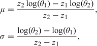where z₁ and z₂ are the p₁ and p₂ quantiles of a standard normal random variable. For example, in an epidemiological context, we may wish to specify a prior on a relative risk parameter, exp(β₁), which has a median of 1 and a 95% point of 3 (if we think it is unlikely that the relative risk associated with a unit increase in exposure exceeds 3). These specifications lead to β₁ ∼ N(0,0.668²).

4.2. Variance components

We begin by describing an approach for choosing a prior for a single random effect, based on Wakefield (2009). The basic idea is to specify a range for the more interpretable marginal distribution of b_i and use this to drive specification of prior parameters. We state a trivial lemma upon which prior specification is based, but first define some notation. We write τ ∼ Ga(a₁,a₂) for the gamma distribution with unnormalized density τ^{a₁ − 1}exp( − a₂τ). For q-dimensional x, we write x ∼ T_q(μ,Ω,d) for the Student's t distribution with unnormalized density [1 + (x − μ)^TΩ ^{− 1}(x − μ)/d] ^{− (d + q)/2}. This distribution has location μ, scale matrix Ω, and degrees of freedom d.

LEMMA 1

Let b|τ ∼ N(0,τ ^{− 1}) and τ ∼ Ga(a₁,a₂). Integration over τ gives the marginal distribution of b as T₁(0,a₂/a₁,2a₁).

To decide upon a prior, we give a range for a generic random effect b and specify the degrees of freedom, d, and then solve for a₁ and a₂. For the range (−R,R), we use the relationship 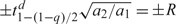, where t_q^d is the 100 × qth quantile of a Student t random variable with d degrees of freedom, to give a₁ = d/2 and a₂ = R²d/2(t_{1 − (1 − q)/2}^d)². In the linear mixed effects model, b is directly interpretable, while for binomial or Poisson models, it is more appropriate to think in terms of the marginal distribution of exp(b), the residual odds and rate ratio, respectively, and this distribution is log Student's t. For example, if we choose d = 1 (to give a Cauchy marginal) and a 95% range of [0.1,10], we take R = log10 and obtain a = 0.5 and b = 0.0164.

Another convenient choice is d = 2 to give the exponential distribution with mean a₂⁻¹ for σ⁻². This leads to closed-form expressions for the more interpretable quantiles of σ so that, for example, if we specify the median for σ as σ_m, we obtain a₂ = σ_m²log2.

Unfortunately, the use of Ga(ϵ,ϵ) priors has become popular as a prior for σ⁻² in a GLMM context, arising from their use in the winBUGS examples manual. As has been pointed out many times (e.g. Kelsall and Wakefield, 1999, Gelman, 2006, Crainiceanu and others, 2008), this choice places the majority of the prior mass away from zero and leads to a marginal prior for the random effects which is Student's t with 2ϵ degrees of freedom (so that the tails are much heavier than even a Cauchy) and difficult to justify in any practical setting.

We now specify another trivial lemma, but first establish notation for the Wishart distribution. For the q × q nonsingular matrix z, we write z ∼ Wishart_q(r,S) for the Wishart distribution with unnormalized density . This distribution has E[z] = rS and E[z ^{− 1}] = S ^{− 1}/(r − q − 1), and we require r > q − 1 for a proper distribution.

Lemma:

Let b = (b₁,…,b_q), with b|Q ∼ _iidN_q(0,Q ^{− 1}), Q ∼ Wishart_q(r,S). Integration over Q gives the marginal distribution of b as T_q(0,[(r − q + 1)S] ^{− 1},r − q + 1).

The margins of a multivariate Student's t are t also, which allows r and S to be chosen as in the univariate case. Specifically, the kth element of a generic random effect, b_k, follows a univariate Student t distribution with location 0, scale S^kk/(r − q + 1), and degrees of freedom d = r − q + 1, where S^kk is element (k,k) of the inverse of S. We obtain r = d + q − 1 and S^kk = (t_{1 − (1 − q)/2}^d)²/(dR²). If a priori we have no reason to believe that elements of b are correlated we may specify S_jk = 0 for j ≠ k and S^kk = 1/S_kk, to recover the univariate specification, recognizing that with q = 1, the univariate Wishart has parameters a₁ = r/2 and a₂ = 1/(2S). If we believe that elements of b are dependent then we may specify the correlations and solve for the off-diagonal elements of S. To ensure propriety of the posterior, proper priors are required for Σ; Zeger and Karim (1991) use an improper prior for Σ, so that the posterior is improper also.

4.3. Effective degrees of freedom variance components prior

In Section 5.3, we describe the GLMM representation of a spline model. A generic linear spline model is given by

where x_i is a p × 1 vector of covariates with p × 1 associated fixed effects β, z_ik denote the spline basis, b_k ∼ _iidN(0,σ_b²), and ϵ_i ∼ _iidN(0,σ_ϵ²), with b_k and ϵ_i independent. Specification of a prior for σ_b² is not straightforward, but may be of great importance since it contributes to determining the amount of smoothing that is applied. Ruppert and others (p. 177 2003) raise concerns, “about the instability of automatic smoothing parameter selection even for single predictor models”, and continue, “Although we are attracted by the automatic nature of the mixed model-REML approach to fitting additive models, we discourage blind acceptance of whatever answer it provides and recommend looking at other amounts of smoothing”. While we would echo this general advice, we believe that a Bayesian mixed model approach, with carefully chosen priors, can increase the stability of the mixed model representation. There has been some discussion of choice of prior for σ_b² in a spline context (Crainiceanu and others, 2005), (Crainiceanu and others, 2008). More general discussion can be found in Natarajan and Kass (2000) and Gelman (2006).

In practice (e.g. Hastie and Tibshirani, 1990), smoothers are often applied with a fixed degrees of freedom. We extend this rationale by examining the prior degrees of freedom that is implied by the choice σ_b ^{− 2} ∼ Ga(a₁,a₂). For the general linear mixed model

we have

where C = [x|z] is n × (p + K) and

(see, e.g. Ruppert and others, 2003). The total degrees of freedom associated with the model is

which may be decomposed into the degrees of freedom associated with β and b, and extends easily to situations in which we have additional random effects, beyond those associated with the spline basis (such an example is considered in Section 5.3). In each of these situations, the degrees of freedom associated with the respective parameter is obtained by summing the appropriate diagonal elements of (C^TC + Λ) ^{− 1}C^TC. Specifically, if we have j = 1,…,d sets of random-effect parameters (there are d = 2 in the model considered in Section 5.3) then let E_j be the (p + K) × (p + K) diagonal matrix with ones in the diagonal positions corresponding to set j. Then the degrees of freedom associated with this set is df_j = tr{E_j(C^TC + Λ) ^{− 1}C^TC. Note that the effective degrees of freedom changes as a function of K, as expected. To evaluate Λ, σ_ϵ² is required. If we specify a proper prior for σ_ϵ², then we may specify the joint prior as π(σ_b²,σ_ϵ²) = π(σ_ϵ²)π(σ_b²|σ_ϵ²). Often, however, we assume the improper prior π(σ_ϵ²) ∝ 1/σ_ϵ² since the data provide sufficient information with respect to σ_ϵ². Hence, we have found the substitution of an estimate for σ_ϵ² (for example, from the fitting of a spline model in a likelihood implementation) to be a practically reasonable strategy.

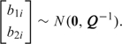
As a simple nonspline demonstration of the derived effective degrees of freedom, consider a 1-way analysis of variance model

with b_i ∼_iidN(0,σ_b²), ϵ_ij ∼_iidN(0,σ_ϵ²) for i = 1,…,m = 10 groups and j = 1,…,n = 5 observations per group. For illustration, we assume σ_b ^{− 2} ∼ Ga(0.5,0.005). Figure 1 displays the prior distribution for σ, the implied prior distribution on the effective degrees of freedom, and the bivariate plot of these quantities. For clarity of plotting, we exclude a small number of points beyond σ > 2.5 (4% of points). In panel (c), we have placed dashed horizontal lines at effective degrees of freedom equal to 1 (complete smoothing) and 10 (no smoothing). From panel (b), we conclude that here the prior choice favors quite strong smoothing. This may be contrasted with the gamma prior with parameters (0.001,0.001), which, in this example, gives greater than 99% of the prior mass on an effective degrees of freedom greater than 9.9, again showing the inappropriateness of this prior.

Fig. 1.

Gamma prior for σ ^{− 2} with parameters 0.5 and 0.005, (a) implied prior for σ, (b) implied prior for the effective degrees of freedom, and (c) effective degrees of freedom versus σ.

It is appealing to extend the above argument to nonlinear models but unfortunately this is not straightforward. For a nonlinear model, the degrees of freedom may be approximated by

where and h = g ^{− 1} denotes the inverse link function. Unfortunately, this quantity depends on β and b, which means that in practice, we would have to use prior estimates for all of the parameters, which may not be practically possible. Fitting the model using likelihood and then substituting in estimates for β and b seems philosophically dubious.

4.4. Random walk models

Conditionally represented smoothing models are popular for random effects in both temporal and spatial applications (see, e.g. Besag and others, 1995, Rue and Held, 2005). For illustration, consider models of the form

(4.1)

where u = (u₁,…,u_m) is the collection of random effects, Q is a (scaled) “precision” matrix of rank m − r, whose form is determined by the application at hand, and |Q^☆| is a generalized determinant which is the product over the m − r nonzero eigenvalues of Q. Picking a prior for σ_u is not straightforward because σ_u has an interpretation as the conditional standard deviation, where the elements that are conditioned upon depends on the application. We may simulate realizations from (4.1) to examine candidate prior distributions. Due to the rank deficiency, (4.1) does not define a probability density, and so we cannot directly simulate from this prior. However, Rue and Held (2005) give an algorithm for generating samples from (4.1):

1. Simulate z_j ∼ N(0,λ_j ^{− 1}), for j = m − r + 1,…,m, where λ_j are the eigenvalues of Q (there are m − r nonzero eigenvalues as Q has rank m − r).

2. Return u = z_{m − r + 1}e_{n − r + 1} + z₃e₃ + ⋯ + z_ne_m = Ez, where e_j are the corresponding eigenvectors of Q, E is the m × (m − r) matrix with these eigenvectors as columns, and z is the (m − r) × 1 vector containing z_j, j = m − r + 1,…,m.

The simulation algorithm is conditioned so that samples are zero in the null-space of Q; if u is a sample and the null-space is spanned by v₁ and v₂, then u^Tv₁ = u^Tv₂ = 0. For example, suppose Q1 = 0 so that the null-space is spanned by 1, and the rank deficiency is 1. Then Q is improper since the eigenvalue corresponding to 1 is zero, and samples u produced by the algorithm are such that u^T1 = 0. In Section 5.2, we use this algorithm to evaluate different priors via simulation. It is also useful to note that if we wish to compute the marginal variances only, simulation is not required, as they are available as the diagonal elements of the matrix ∑_jλ_j ^{− 1}e_je_j^T.

5. EXAMPLES

Here, we report 3 examples, with 4 others described in the supplementary material available at Biostatistics online. Together these cover all the examples in Breslow and Clayton (1993), along with an additional spline example. In the first example, results using the INLA numerical/analytical approximation described in Section 3 were compared with MCMC as implemented in the JAGS software (Plummer, 2009) and found to be accurate. For the models considered in the second and third examples, the approximation was compared with the MCMC implementation contained in the INLA software.

5.1. Longitudinal data

We consider the much analyzed epilepsy data set of Thall and Vail (1990). These data concern the number of seizures, Y_ij for patient i on visit j, with Y_ij|β,b_i ∼ _indPoisson(μ_ij), i = 1,…,59, j = 1,…,4. We concentrate on the 3 random-effects models fitted by Breslow and Clayton (1993):

(5.1)

(5.2)

(5.3)

where x_ij is a 1 × 6 vector containing a 1 (representing the intercept), an indicator for baseline measurement, a treatment indicator, the baseline by treatment interaction, which is the parameter of interest, age, and either an indicator of the fourth visit (models (5.1) and (5.2) and denoted V₄) or visit number coded − 3, − 1, + 1, + 3 (model (5.3) and denoted V_j/10) and β is the associated fixed effect. All 3 models include patient-specific random effects b_1i ∼ N(0,σ₁²), while in model (5.2), we introduce independent “measurement errors,” b_0ij ∼ N(0,σ₀²). Model (5.3) includes random effects on the slope associated with visit, b_2i with

(5.4)

We assume Q ∼ Wishart(r,S) with For prior specification, we begin with the bivariate model and assume that S is diagonal. We assume the upper 95% point of the priors for exp(b_1i) and exp(b_2i) are 5 and 4, respectively, and that the marginal distributions are t with 4 degrees of freedom. Following the procedure outlined in Section 4.2, we obtain r = 5 and S = diag(0.439,0.591). We take the prior for σ₁ ^{− 2} in model (5.1) to be Ga(a₁,a₂) with a₁ = (r − 1)/2 = 2 and a₂ = 1/2S₁₁ = 1.140 (so that this prior coincides with the marginal prior obtained from the bivariate specification). In model (5.2), we assume b_1i and b_0ij are independent, and that σ₀ ^{− 2} follows the same prior as σ₁ ^{− 2}, that is, Ga(2,1.140). We assume a flat prior on the intercept, and assume that the rate ratios, exp(β_j), j = 1,…,5, lie between 0.1 and 10 with probability 0.95 which gives, using the approach described in Section 4.1, a normal prior with mean 0 and variance 1.17².

Table 1 gives PQL and INLA summaries for models (5.1–5.3). There are some differences between the PQL and Bayesian analyses, with slightly larger standard deviations under the latter, which probably reflects that with m = 59 clusters, a little accuracy is lost when using asymptotic inference. There are some differences in the point estimates which is at least partly due to the nonflat priors used—the priors have relatively large variances, but here the data are not so abundant so there is sensitivity to the prior. Reassuringly under all 3 models inference for the baseline-treatment interaction of interest is virtually identical and suggests no significant treatment effect. We may compare models using logp(y): for 3 models, we obtain values of − 674.8, − 638.9, and − 665.5, so that the second model is strongly preferred.

Table 1.

PQL and INLA summaries for the epilepsy data

	Model (5.1)		Model (5.2)		Model (5.3)
Variable	PQL	INLA	PQL	INLA	PQL	INLA
Base	0.87 ± 0.14	0.88 ± 0.15	0.86 ± 0.13	0.88 ± 0.15	0.87 ± 0.14	0.88 ± 0.14
Trt	− 0.91 ± 0.41	− 0.94 ± 0.44	− 0.93 ± 0.40	− 0.96 ± 0.44	− 0.91 ± 0.41	− 0.94 ± 0.44
Base × Trt	0.33 ± 0.21	0.34 ± 0.22	0.34 ± 0.21	0.35 ± 0.23	0.33 ± 0.21	0.34 ± 0.22
Age	0.47 ± 0.36	0.47 ± 0.38	0.47 ± 0.35	0.48 ± 0.39	0.46 ± 0.36	0.47 ± 0.38
V4 or V/10	− 0.16 ± 0.05	− 0.16 ± 0.05	− 0.10 ± 0.09	− 0.10 ± 0.09	− 0.26 ± 0.16	− 0.27 ± 0.16
σ0	—	—	0.36 ± 0.04	0.41 ± 0.04	—	—
σ1	0.53 ± 0.06	0.56 ± 0.08	0.48 ± 0.06	0.53 ± 0.07	0.52 ± 0.06	0.56 ± 0.06
σ2	—	—	—	—	0.74 ± 0.16	0.70 ± 0.14

5.2. Smoothing of birth cohort effects in an age-cohort model

We analyze data from Breslow and Day (1975) on breast cancer rates in Iceland. Let Y_jk be the number of breast cancer of cases in age group j (20–24,…,80–84) and birth cohort k (1840–1849,…,1940–1949) with j = 1,…,J = 13 and k = 1,…,K = 11. Following Breslow and Clayton (1993), we assume Y_jk|μ_jk ∼ _indPoisson(μ_jk) with

(5.5)

and where n_jk is the person-years denominator, exp(β_j),j = 1,…,J, represent fixed effects for age relative risks, exp(β) is the relative risk associated with a one group increase in cohort group, v_k ∼ _iidN(0,σ_v²) represent unstructured random effects associated with cohort k, with smooth cohort terms u_k following a second-order random-effects model with E[u_k|{u_i:i < k}] = 2u_{k − 1} − u_{k − 2} and Var(u_k|{u_i:i < k}) = σ_u². This latter model is to allow the rates to vary smoothly with cohort. An equivalent representation of this model is, for 2 < k < K − 1,

The rank of Q in the (4.1) representation of this model is K − 2 reflecting that both the overall level and the overall trend are aliased (hence the appearance of β in (5.5)).

The term exp(v_k) reflects the unstructured residual relative risk and, following the argument in Section 4.2, we specify that this quantity should lie in [0.5,2.0] with probability 0.95, with a marginal log Cauchy distribution, to obtain the gamma prior σ_v ^{− 2} ∼ Ga(0.5,0.00149).

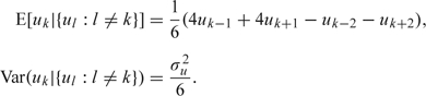
The term exp(u_k) reflects the smooth component of the residual relative risk, and the specification of a prior for the associated variance component σ_u² is more difficult, given its conditional interpretation. Using the algorithm described in Section 4.2, we examined simulations of u for different choices of gamma hyperparameters and decided on the choice σ_u ^{− 2} ∼ Ga(0.5,0.001); Figure 2 shows 10 realizations from the prior. The rationale here is to examine realizations to see if they conform to our prior expectations and in particular exhibit the required amount of smoothing. All but one of the realizations vary smoothly across the 11 cohorts, as is desirable. Due to the tail of the gamma distribution, we will always have some extreme realizations.

Fig. 2.

(a) Ten realizations (on the relative risk scale) from the random effects second-order random walk model in which the prior on the random-effects precision is Ga(0.5,0.001), (b) summaries of fitted models: the solid line corresponds to a log-linear model in birth cohort, the circles to birth cohort as a factor, and “+” to the Bayesian smoothing model.

The INLA results, summarized in graphical form, are presented in Figure 2(b), alongside likelihood fits in which the birth cohort effect is incorporated as a linear term and as a factor. We see that the smoothing model provides a smooth fit in birth cohort, as we would hope.

5.3. B-Spline nonparametric regression

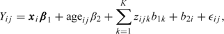
We demonstrate the use of INLA for nonparametric smoothing using O'Sullivan splines, which are based on a B-spline basis. We illustrate using data from Bachrach and others (1999) that concerns longitudinal measurements of spinal bone mineral density (SBMD) on 230 female subjects aged between 8 and 27, and of 1 of 4 ethnic groups: Asian, Black, Hispanic, and White. Let y_ij denote the SBMD measure for subject i at occasion j, for i = 1,…,230 and j = 1,…,n_i with n_i being between 1 and 4. Figure 3 shows these data, with the gray lines indicating measurements on the same woman.

Fig. 3.

SBMD versus age by ethnicity. Measurements on the same woman are joined with gray lines. The solid curve corresponds to the fitted spline and the dashed lines to the individual fits.

We assume the model

where x_i is a 1 × 4 vector containing an indicator for the ethnicity of individual i, with β₁ the associated 4 × 1 vector of fixed effects, z_ijk is the kth basis associated with age, with associated parameter b_1k ∼ N(0,σ₁²), and b_2i ∼ N(0,σ₂²) are woman-specific random effects, finally, ϵ_ij ∼ _iidN(0,σ_ϵ²). All random terms are assumed independent. Note that the spline model is assumed common to all ethnic groups and all women, though it would be straightforward to allow a different spline for each ethnicity. Writing this model in the form

we use the method described in Section 4.3 to examine the effective number of parameters implied by the priors σ₁⁻² ∼ Ga(a₁,a₂) and σ₂⁻² ∼ Ga(a₃,a₄).

To fit the model, we first use the R code provided in Wand and Ormerod (2008) to construct the basis functions, which are then input to the INLA program. Running the REML version of the model, we obtain which we use to evaluate the effective degrees of freedoms associated with priors for σ₁² and σ₂². We assume the usual improper prior, π(σ_ϵ²) ∝ 1/σ_ϵ² for σ_ϵ². After some experimentation, we settled on the prior σ₁ ^{− 2} ∼ Ga(0.5,5 × 10 ^{− 6}). For σ₂², we wished to have a 90% interval for b_2i of ±0.3 which, with 1 degree of freedom for the marginal distribution, leads to σ₂⁻² ∼ Ga(0.5,0.00113). Figure 4 shows the priors for σ₁ and σ₂, along with the implied effective degrees of freedom under the assumed priors. For the spline component, the 90% prior interval for the effective degrees of freedom is [2.4,10].

Fig. 4.

Prior summaries: (a) σ₁, the standard deviation of the spline coefficients, (b) effective degrees of freedom associated with the prior for the spline coefficients, (c) effective degrees of freedom versus σ₁, (d) σ₂, the standard deviation of the between-individual random effects, (e) effective degrees of freedom associated with the individual random effects, and (f) effective degrees of freedom versus σ₂. The vertical dashed lines on panels (a), (b), (d), and (e) correspond to the posterior medians.

Table 2 compares estimates from REML and INLA implementations of the model, and we see close correspondence between the 2. Figure 4 also shows the posterior medians for σ₁ and σ₂ and for the 2 effective degrees of freedom. For the spline and random effects these correspond to 8 and 214, respectively. The latter figure shows that there is considerable variability between the 230 women here. This is confirmed in Figure 3 where we observe large vertical differences between the profiles. This figure also shows the fitted spline, which appears to mimic the trend in the data well.

Table 2.

REML and INLA summaries for spinal bone data. Intercept corresponds to Asian group.

Variable	REML	INLA
Intercept	0.560 ± 0.029	0.563 ± 0.031
Black	0.106 ± 0.021	0.106 ± 0.021
Hispanic	0.013 ± 0.022	0.013 ± 0.022
White	0.026 ± 0.022	0.026 ± 0.022
Age	0.021 ± 0.002	0.021 ± 0.002
σ1	0.018★	0.024 ± 0.006
σ2	0.109★	0.109 ± 0.006
σϵ	0.033★	0.033 ± 0.002

Note: For the entries marked with a^★ standard errors were unavailable.

5.4. Timings

For the 3 models in the longitudinal data example, INLA takes 1 to 2 s to run, using a single CPU. To get estimates with similar precision with MCMC, we ran JAGS for 100 000 iterations, which took 4 to 6 min. For the model in the temporal smoothing example, INLA takes 45 s to run, using 1 CPU. Part of the INLA procedure can be executed in a parallel manner. If there are 2 CPUs available, as is the case with today's prevalent INTEL Core 2 Duo processors, INLA only takes 27 s to run. It is not currently possible to implement this model in JAGS. We ran the MCMC utility built into the INLA software for 3.6 million iterations, to obtain estimates of comparable accuracy, which took 15 h. For the model in the B-spline nonparametric regression example, INLA took 5 s to run, using a single CPU. We ran the MCMC utility built into the INLA software for 2.5 million iterations to obtain estimates of comparable accuracy, the analysis taking 40 h.

6. DISCUSSION

In this paper, we have demonstrated the use of the INLA computational method for GLMMs. We have found that the approximation strategy employed by INLA is accurate in general, but less accurate for binomial data with small denominators. The supplementary material available at Biostatistics online contains an extensive simulation study, replicating that presented in Breslow and Clayton (1993). There are some suggestions in the discussion of Rue and others (2009) on how to construct an improved Gaussian approximation that does not use the mode and the curvature at the mode. It is likely that these suggestions will improve the results for binomial data with small denominators. There is an urgent need for diagnosis tools to flag when INLA is inaccurate. Conceptually, computation for nonlinear mixed effects models (Davidian and Giltinan, 1995), (Pinheiro and Bates, 2000) can also be handled by INLA but this capability is not currently available.

The website www.r-inla.org contains all the data and R scripts to perform the analyses and simulations reported in the paper. The latest release of software to implement INLA can also be found at this site. Recently, Breslow (2005) revisited PQL and concluded that, “PQL still performs remarkably well in comparison with more elaborate procedures in many practical situations.” We believe that INLA provides an attractive alternative to PQL for GLMMs, and we hope that this paper stimulates the greater use of Bayesian methods for this class.

SUPPLEMENTARY MATERIAL

Supplementary material is available at http://biostatistics.oxfordjournals.org.

FUNDING

National Institutes of Health (R01 CA095994) to J.W. Statistics for Innovation (sfi.nr.no) to H.R.

Conflict of Interest: None declared.

References

- Bachrach LK, Hastie T, Wang MC, Narasimhan B, Marcus R. Bone mineral acquisition in healthy Asian, Hispanic, Black and Caucasian youth. A longitudinal study. The Journal of Clinical Endocrinology and Metabolism. 1999;84:4702–4712. doi: 10.1210/jcem.84.12.6182. [DOI] [PubMed] [Google Scholar]
- Besag J, Green PJ, Higdon D, Mengersen K. Bayesian computation and stochastic systems (with discussion) Statistical Science. 1995;10:3–66. [Google Scholar]
- Breslow NE. Whither PQL? In: Lin D, Heagerty PJ, editors. Proceedings of the Second Seattle Symposium. New York: Springer; 2005. pp. 1–22. [Google Scholar]
- Breslow NE, Clayton DG. Approximate inference in generalized linear mixed models. Journal of the American Statistical Association. 1993;88:9–25. [Google Scholar]
- Breslow NE, Day NE. Indirect standardization and multiplicative models for rates, with reference to the age adjustment of cancer incidence and relative frequency data. Journal of Chronic Diseases. 1975;28:289–301. doi: 10.1016/0021-9681(75)90010-7. [DOI] [PubMed] [Google Scholar]
- Clayton DG. Generalized linear mixed models. In: Gilks WR, Richardson S, Spiegelhalter DJ, editors. Markov Chain Monte Carlo in Practice. London: Chapman and Hall; 1996. pp. 275–301. [Google Scholar]
- Crainiceanu CM, Diggle PJ, Rowlingson B. Bayesian analysis for penalized spline regression using winBUGS. Journal of the American Statistical Association. 2008;102:21–37. [Google Scholar]
- Crainiceanu CM, Ruppert D, Wand MP. Bayesian analysis for penalized spline regression using winBUGS. Journal of Statistical Software. 2005:14. [Google Scholar]
- Davidian M, Giltinan DM. Nonlinear Models for Repeated Measurement Data. London: Chapman and Hall; 1995. [Google Scholar]
- DiCiccio TJ, Kass RE, Raftery A, Wasserman L. Computing Bayes factors by combining simulation and asymptotic approximations. Journal of the American Statistical Association. 1997;92:903–915. [Google Scholar]
- Diggle P, Heagerty P, Liang K-Y, Zeger S. Analysis of Longitudinal Data. 2nd edition. Oxford: Oxford University Press; 2002. [Google Scholar]
- Fahrmeir L, Kneib T, Lang S. Penalized structured additive regression for space-time data: a Bayesian perspective. Statistica Sinica. 2004;14:715–745. [Google Scholar]
- Gamerman D. Sampling from the posterior distribution in generalized linear mixed models. Statistics and Computing. 1997;7:57–68. [Google Scholar]
- Gelman A. Prior distributions for variance parameters in hierarchical models. Bayesian Analysis. 2006;1:515–534. [Google Scholar]
- Hastie TJ, Tibshirani RJ. Generalized Additive Models. London: Chapman and Hall; 1990. [Google Scholar]
- Hobert JP, Casella G. The effect of improper priors on Gibbs sampling in hierarchical linear mixed models. Journal of the American Statistical Association. 1996;91:1461–1473. [Google Scholar]
- Kass RE, Steffey D. Approximate Bayesian inference in conditionally independent hierarchical models (parametric empirical Bayes models) Journal of the American Statistical Association. 1989;84:717–726. [Google Scholar]
- Kelsall JE, Wakefield JC. Discussion of “Bayesian models for spatially correlated disease and exposure data” by N. Best, I. Waller, A. Thomas, E. Conlon and R. Arnold. In: Bernardo JM, Berger JO, Dawid AP, Smith AFM, editors. Sixth Valencia International Meeting on Bayesian Statistics. London: Oxford University Press; 1999. [Google Scholar]
- McCullagh P, Nelder JA. Generalized Linear Models. 2nd edition. London: Chapman and Hall; 1989. [Google Scholar]
- McCulloch CE, Searle SR, Neuhaus JM. Generalized, Linear, and Mixed Models. 2nd edition. New York: John Wiley and Sons; 2008. [Google Scholar]
- Meng X, Wong W. Simulating ratios of normalizing constants via a simple identity. Statistical Sinica. 1996;6:831–860. [Google Scholar]
- Natarajan R, Kass RE. Reference Bayesian methods for generalized linear mixed models. Journal of the American Statistical Association. 2000;95:227–237. [Google Scholar]
- Nelder J, Wedderburn R. Generalized linear models. Journal of the Royal Statistical Society, Series A. 1972;135:370–384. [Google Scholar]
- Pinheiro JC, Bates DM. Mixed-Effects Models in S and S-plus. New York: Springer; 2000. [Google Scholar]
- Plummer M. Penalized loss functions for Bayesian model comparison. Biostatistics. 2008;9:523–539. doi: 10.1093/biostatistics/kxm049. [DOI] [PubMed] [Google Scholar]
- Plummer M. Jags version 1.0.3 manual. Technical Report. 2009 [Google Scholar]
- Rue H, Held L. Gaussian Markov Random Fields: Thoery and Application. Boca Raton: Chapman and Hall/CRC; 2005. [Google Scholar]
- Rue H, Martino S, Chopin N. Approximate Bayesian inference for latent Gaussian models using integrated nested laplace approximations (with discussion) Journal of the Royal Statistical Society, Series B. 2009;71:319–392. [Google Scholar]
- Ruppert DR, Wand MP, Carroll RJ. Semiparametric Regression. New York: Cambridge University Press; 2003. [Google Scholar]
- Skene AM, Wakefield JC. Hierarchical models for multi-centre binary response studies. Statistics in Medicine. 1990;9:919–929. doi: 10.1002/sim.4780090808. [DOI] [PubMed] [Google Scholar]
- Spiegelhalter D, Best N, Carlin B, van der Linde A. Bayesian measures of model complexity and fit (with discussion) Journal of the Royal Statistical Society, Series B. 1998;64:583–639. [Google Scholar]
- Spiegelhalter DJ, Thomas A, Best NG. WinBUGS User Manual. 1998. Version 1.1.1. Cambridge. [Google Scholar]
- Thall PF, Vail SC. Some covariance models for longitudinal count data with overdispersion. Biometrics. 1990;46:657–671. [PubMed] [Google Scholar]
- Verbeke G, Molenberghs G. Linear Mixed Models for Longitudinal Data. New York: Springer; 2000. [Google Scholar]
- Verbeke G, Molenberghs G. Models for Discrete Longitudinal Data. New York: Springer; 2005. [Google Scholar]
- Wakefield JC. Disease mapping and spatial regression with count data. Biostatistics. 2007;8:158–183. doi: 10.1093/biostatistics/kxl008. [DOI] [PubMed] [Google Scholar]
- Wakefield JC. Multi-level modelling, the ecologic fallacy, and hybrid study designs. International Journal of Epidemiology. 2009;38:330–336. doi: 10.1093/ije/dyp179. [DOI] [PMC free article] [PubMed] [Google Scholar]
- Wand MP, Ormerod JT. On semiparametric regression with O'Sullivan penalised splines. Australian and New Zealand Journal of Statistics. 2008;50:179–198. [Google Scholar]
- Zeger SL, Karim MR. Generalized linear models with random effects: a Gibbs sampling approach. Journal of the American Statistical Association. 1991;86:79–86. [Google Scholar]
Associated Data
This section collects any data citations, data availability statements, or supplementary materials included in this article.