Improving Polyp Detection Algorithms for CT Colonography: Pareto Front Approach

Abstract

We investigated a Pareto front approach to improving polyp detection algorithms for CT colonography (CTC). A dataset of 56 CTC colon surfaces with 87 proven positive detections of 53 polyps sized 4 to 60 mm was used to evaluate the performance of a one-step and a two-step curvature-based region growing algorithm. The algorithmic performance was statistically evaluated and compared based on the Pareto optimal solutions from 20 experiments by evolutionary algorithms. The false positive rate was lower (p<0.05) by the two-step algorithm than by the one-step for 63% of all possible operating points. While operating at a suitable sensitivity level such as 90.8% (79/87) or 88.5% (77/87), the false positive rate was reduced by 24.4% (95% confidence intervals 17.9–31.0%) or 45.8% (95% confidence intervals 40.1–51.0%) respectively. We demonstrated that, with a proper experimental design, the Pareto optimization process can effectively help in fine-tuning and redesigning polyp detection algorithms.

1. INTRODUCTION

Colonic polyps are abnormal growths that originate from cells of the colonic mucosa, the inner wall of the colon. Most are benign but some (adenomas) can become cancerous. Finding and removing polyps can reduce the risk of colorectal cancer (Winawer et al., 1993). Computed tomographic colonography (CTC) is a new, less invasive screening technique that has shown promising results (Hara et al., 1997; Yee et al., 2001; Pickhardt et al., 2003). However, variable sensitivity among readers needs to be resolved before CTC is put into widespread use (Cotton et al., 2004; Rockey et al., 2005). In order to reduce inter-observer variability and improve sensitivity in detecting small polyps, several computer-aided detection (CAD) systems for CTC have been introduced (Summers et al., 2000; Yoshida and Nappi, 2001; Paik et al., 2004; Mani et al., 2005; Summers et al., 2005; Melonakos et al., 2007; Mendonca et al., 2008). As the CTC CAD development has progressed in the past few years (Yoshida and Dachman, 2005; Bielen and Kiss, 2007), software has grown more sophisticated and it has become more challenging to improve such an increasingly complex system.

CAD is a multi-step procedure consisting of two major algorithmic components: image processing and feature analysis. Functions such as colon wall segmentation (Chen et al., 2000; Masutani et al., 2001; Frimmel et al., 2005; Franaszek et al., 2006), polyp candidate localization (Summers et al., 2000; Yoshida and Nappi, 2001; Paik et al., 2004; Yao et al., 2004; Chowdhury et al., 2006; van Wijk et al., 2006; Bhotika et al., 2006; Kiss et al., 2006; Hong et al., 2006), and polyp candidate feature extraction belong to the realm of image processing; feature selection (Sahiner et al., 2000; Li et al., 2006), classification (Chan et al., 1999), and operating point selection belong to the realm of feature analysis. Ideally, the entire CAD system should be optimized as one unit. This approach is not pragmatic due to the computational complexity of the entire algorithm. As most CAD systems are highly modular with interchangeable algorithmic components, one practical approach is to optimize these algorithmic components individually. However, most published work on CAD system optimization has been limited to the feature analysis components and, particularly, to classifiers such as linear discriminant analysis (Wagner et al., 1997), artificial neural network (Kupinski et al, 2001; Jerebko et al., 2003; Kodogiannis et al., 2007), multiobjective optimization (Anastasio et al., 1998; Kupinski and Anastasio, 1999), and support vector machines (Yao et al., 2005; Campadelli et al., 2005). Although there are many polyp candidate localization algorithms available in the literature, little work has been published in evaluating, comparing, or optimizing them. This shortcoming has motivated us to conduct this study.

Polyp candidate localization is an intermediate step which reduces the potential targets from the whole colon to a small number of polyp candidates. As the majority of colonic polyps are elliptical protrusions of the mucosa or pedunculated, shape-based strategies are popular and rather successful. Various strategies have been proposed such as curvature (Summers et al., 2000; Yoshida and Nappi, 2001), surface normal (Paik et al., 2004; Chowdhury et al., 2006), deformable model (Yao et al., 2004; van Wijk et al., 2006), analytical shape model (Bothika et al., 2006), sphere fitting (Kiss et al., 2006), and texture analysis (Hong et al., 2006). Most of these papers only present the methodology and only two papers provide some degree of performance evaluation such as histographic analysis (Summers et al., 2000) and statistical noisy model analysis (Paik et al., 2004). Recently, curvature estimation accuracy for the colon wall has been discussed in (Huang et al., 2005) and (Campbell and Summers, 2007). Stochastic shape modeling and curvature probability distributions of polyps, haustra, and folds are also discussed in (Mendonca et al., 2008) and (Melonakos et al., 2007) for CAD system improvement.

In this paper we investigated a Pareto front approach to evaluating and improving curvature-based region growing algorithms commonly used in polyp candidate localization. A parallel implementation of Pareto fronts on a Linux cluster environment was developed and tested on two well-known curvature-based algorithms (Summers et al., 2000; Yoshida and Nappi, 2001). We attempt to demonstrate that Pareto fronts are applicable tools to compare and improve image processing algorithms for CTC CAD systems, especially when optimizing individual algorithmic components within a CAD algorithm.

2. MATERIALS AND METHODS

2.1 Data

The clinical data set was from a database of previously described CTC data (Summers et al., 2006). CTC was performed on 29 patients with a high suspicion of polyps or masses. Patients underwent a standard oral colonoscopy preparation and air insufflation of the colon to patient tolerance. Patients were scanned both prone and supine; all patients had colonoscopy performed within 2 months of CTC.

CT scans were done on a 4- or 16-row helical CT scanner (Siemens Volume Zoom, Sensation 4 and Sensation 16). CT scanning parameters were 140kVp, routine (nonreduced) tube current (176 mAs mean; range 150–201), field-of-view to fit (29–49 cm), 3-mm collimation, and 1.5-mm reconstruction interval.

Fifty-six colon surfaces from these 29 patients were segmented by using the method described in (Franaszek et al., 2006) and reconstructed by the marching cubes (MC) algorithm. Degenerated triangles produced by the MC method were removed by in-house software. Colon surfaces from both supine and prone scanned positions were available for all but two patients whose prone scan surfaces could not be evaluated. Each patient had at least one colonoscopy proven polyp. In total, there were 5 small (1–5mm), 12 medium (6–9mm), 15 large (10–19mm) polyps; and 21 masses (20mm and above). All polyps and masses were visible in at least one scanned position and they were positively identified at 87 locations on the 56 colon surfaces.

2.2 Curvature-Based Polyp Localization Algorithms

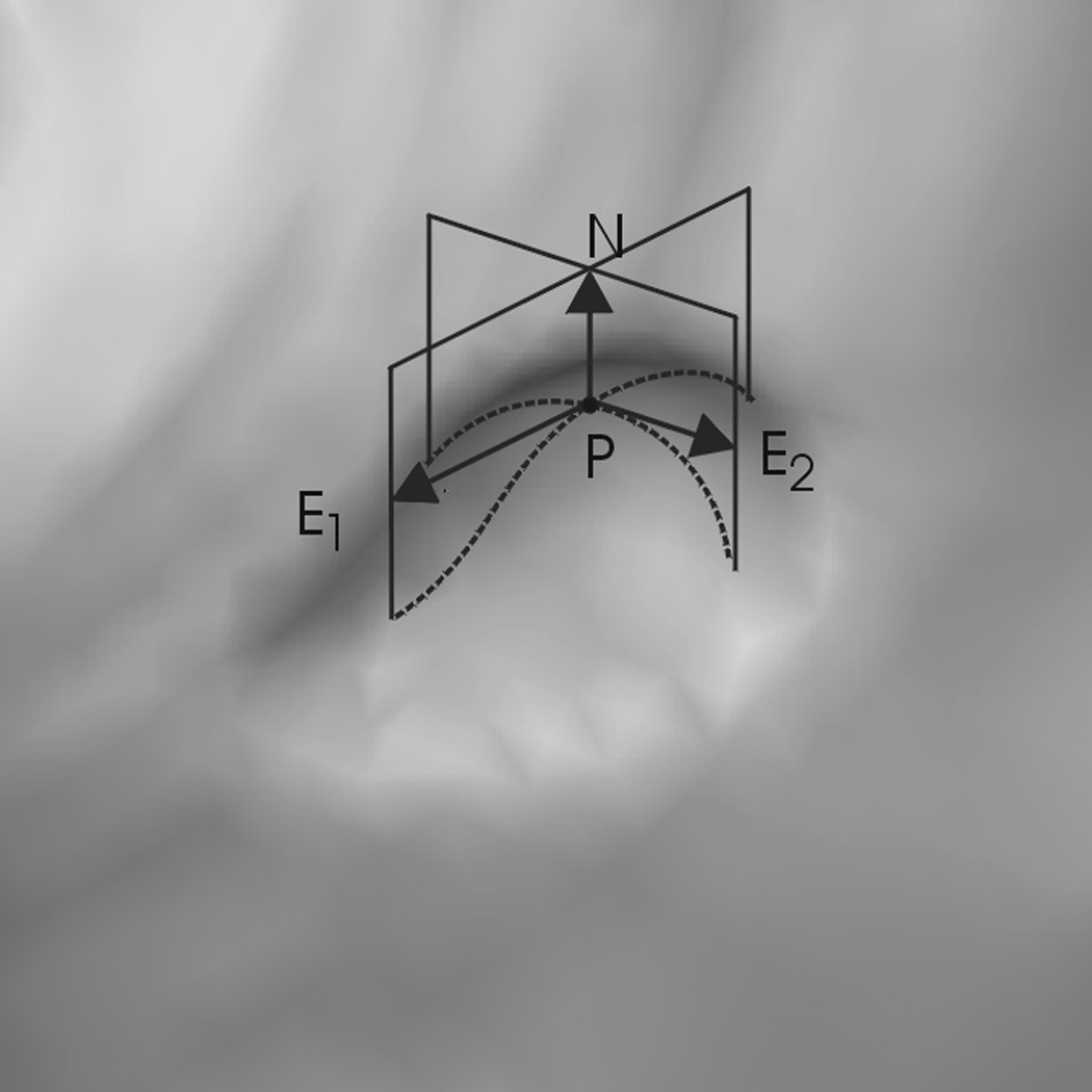
Given air-distended colon surfaces, polyps appear like elliptical protrusions oriented inward toward the colon lumen (Fig. 1). This elliptical feature can be characterized by two principal curvatures which are the maximum and minimum normal curvatures along the principal tangent directions (do Carmo, 1976). Let k₁ and k₂ denote the maximum and minimum principal curvatures respectively and E₁, E₂ their corresponding principal directions which are perpendicular to each other. Polyps can be identified as regions with negative k₁ and k₂ (Huang et al., 2005).By using additional curvature-related properties such as Gaussian curvature K, mean curvature H, and sphericity index SI, polyps can be discriminated from the normal colon surfaces more accurately (Summers et al., 2000). In this paper curvatures k₁ and k₂ were estimated by using the kernel method described in (Campbell and Summers, 2007). Gaussian curvature K and mean curvature H are simply the product (K=k₁k₂) and mean (H=(k₁+k₂)/2) of the two principal curvatures. Sphericity index, SI = |k₁-k₂|/|H|, describes how round an elliptical surface is and ranges from 0 (sphere) to 2 (ridge). Any value in between represents an ellipsoid. Curvature criteria can also be used to classify other colonic structures such as haustra and folds. Readers can refer to (Summers et al., 2000) and (Yoshida and Nappi, 2001) for more information.

Fig. 1.

A 6mm adenomatous polyp appears like an elliptical protrusion. N is the surface normal and E₁ and E₂ are the principal tangent directions at point p.

In this paper two curvature-based region growing algorithms for polyp candidate localization were implemented and compared. The first algorithm, denoted as RA, clusters the vertices satisfying one set of curvature-based criteria on a triangular mesh surface; the second algorithm, denoted as RA+RB, clusters the vertices based on two separate sets of curvature-based criteria. RA was implemented based on (Summers et al., 2000) while RA+RB was a simplified but more adjustable implementation based on the two separate criteria proposed in (Yoshida and Nappi, 2001). In the acronyms RA and RB, R stands for region growing and A/B the criterion set ordered alphabetically. The rationale in devising a new two-criterion region growing algorithm is delineated in the discussion section.

2.2.1 One-Step Region Growing Algorithm RA

The region growing algorithm RA consists of three procedural components: 1) identifying polypoid vertices on colonic surfaces based on a set of curvature characteristics, 2) growing polypoid clusters, and 3) screening the clusters based on member population and shape characteristics.

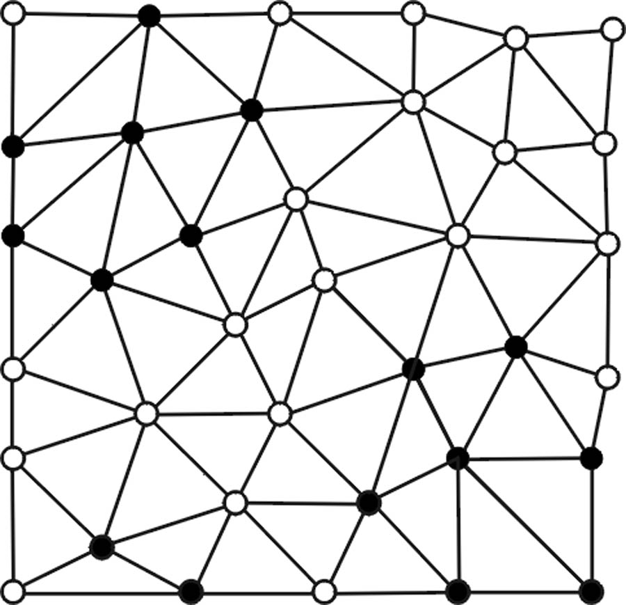
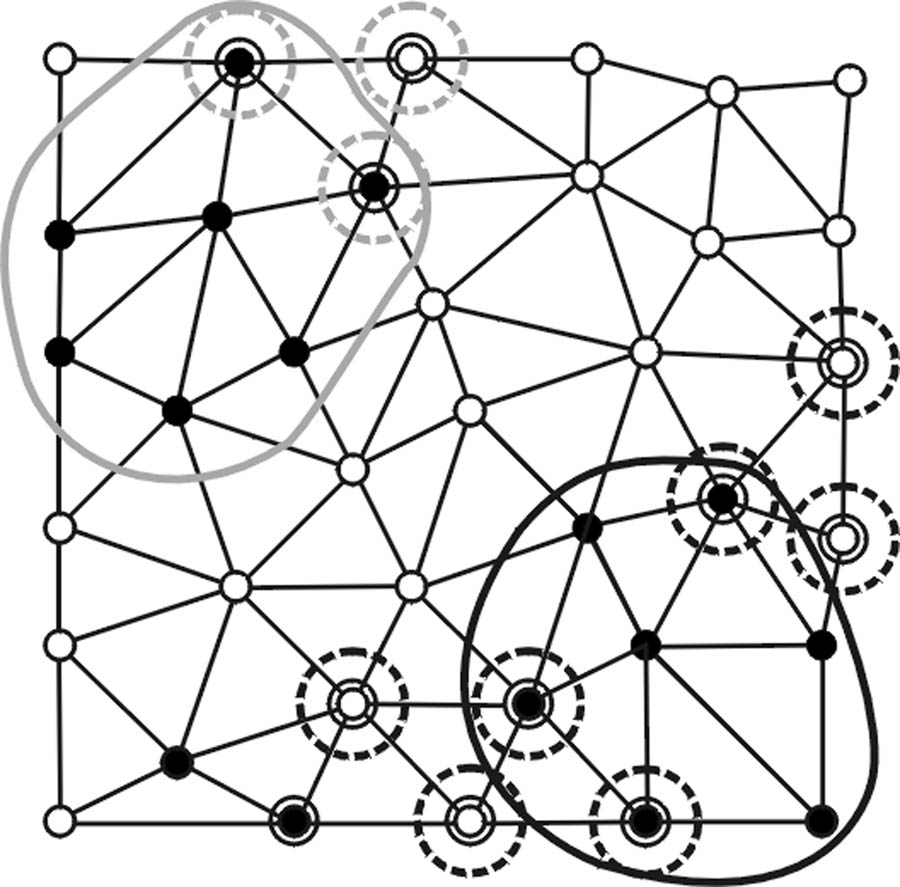
First, letting k₁(p_i), k₂(p_i), H(p_i), and K(p_i) represent the maximum, minimum, mean, and Gaussian curvatures at any vertex p_i on a triangular mesh surface (Fig. 2), polypoid vertices are identified based on three criteria: 1) elliptical criterion: k₁(p_i) < 0 and k₂(p_i) < 0; 2) mean curvature criterion: H_min < H(p_i) < H_max; and 3) Gaussian curvature criterion: K_min < K(p_i) < K_max. H_min, H_max, K_min, and K_min are adjustable operating parameters for shape selectivity. Fig. 2a illustrates an example of resultant polypoid vertices.

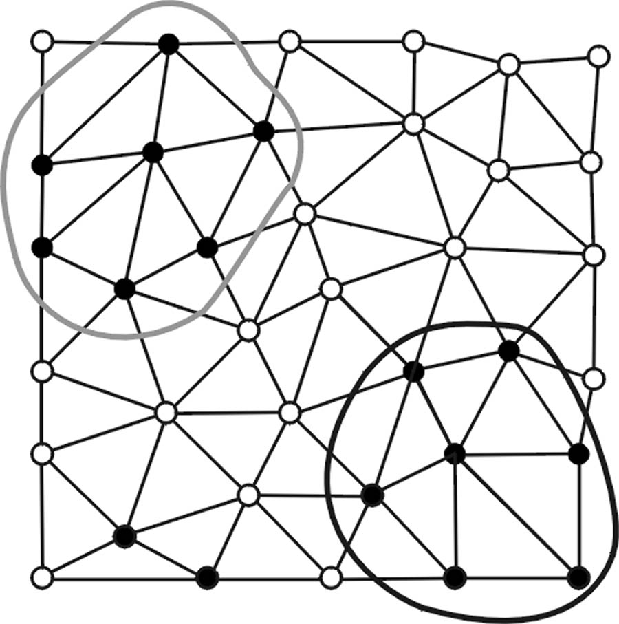
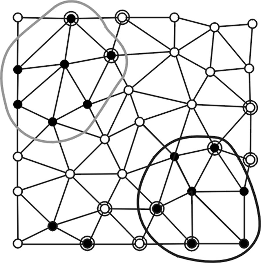
Fig. 2.

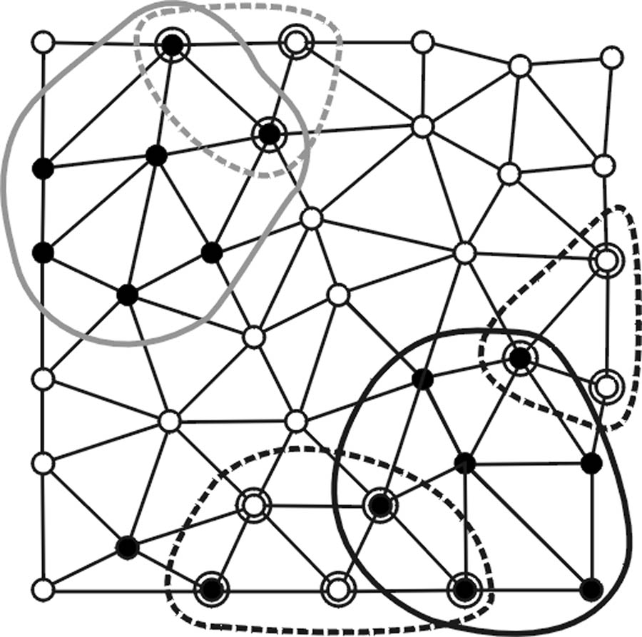
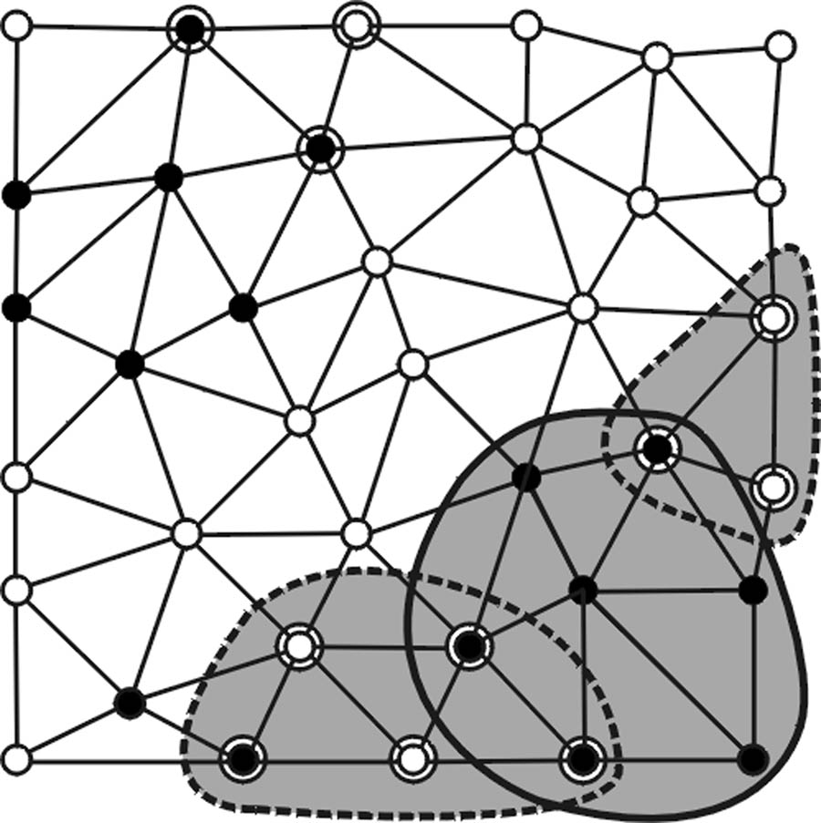
(a) Vertices satisfying a first set of polypoid criteria are denoted as black points. (b) Polypoid vertices form two valid clusters enclosed by the black and gray curves while the black vertices on the lower left area fail to pass the minimum size criterion N_A. (c) Vertices satisfying a secondary set of polypoid criteria are marked by additional circles. (d) New seed points (enclosed by dashed circles) are formed and associated with valid clusters (in corresponding shades). (e) New clusters are formed. (f) Only the cluster (shaded in gray) enclosed by black solid and dashed curves pass the first and second sets of criteria.

Second, neighboring polypoid vertices are then clustered to form disjoint regions based on topological connectivity using regular region growing methods (Huang et al., 2005).

Third, in order to remove noise-induced small bumps and ridge-like folds, the initial clusters are screened based on two additional conditions: the number of vertices in a cluster must be equal to or greater than N_A; and the average sphericity index must be smaller than SI_A. N_A and SI_A are two additional adjustable operating parameters for selectivity.

In summary, algorithm RA forms a set of valid polyp candidates (Fig. 2b) based on a set of adjustable operating parameters (H_min, H_max, K_min, K_max, SI_A, N_A) which is denoted as the one-step criterion vector x_A.

2.2.2 Two-Step Region Growing Algorithm RA+RB

Based on the two separate criteria proposed in (Yoshida and Nappi, 2001), we introduce another algorithm by adding a second region growing step, denoted as RB. The new two-step algorithm is denoted as RA+RB for brevity. The first step of algorithm RA+RB is identical to algorithm RA while the second step, algorithm RB, uses valid polyp candidates found by RA as bases to form new regions via a different set of curvature-based criteria. Algorithm RB consists of four steps.

First, vertices satisfying a different set of three curvature-based criteria are identified (Fig. 2c). They are: 1) elliptical criterion: k₁(p_i) < 0 and k₂(p_i) < 0; 2) mean curvature criterion: H(p_i) < H_B; and 3) spherical criterion: SI(p_i) < SI_B. H_B and SI_B are adjustable operating parameters for different shape selectivity.

Second, polypoid vertices identified in the first step are associated with the clusters formed by RA if they are within valid RA clusters or are their non-member, immediate neighbors (Fig. 2d).

Third, using the associated polypoid vertices found in the second step as the new seed points, a new set of polypoid vertices is formed by applying a regular region growing algorithm. Note that the new polypoid sets shown in Fig. 2e can consist of multiple disconnected vertex clusters since the curvature-based criteria used in algorithms RA and RB are neither inclusive nor exclusive.

Last, the polypoid sets formed in the third step are screened based on a lower vertex population limit N_B (Fig. 2f).

In summary, algorithm RA+RB forms a set of valid polyp candidates based on a set of adjustable operating parameters (H_min, H_max, K_min, K_max, SI_A, N_A, H_B, SI_B, N_B) which is denoted as the two-step criterion vector x_A+B.

2.3 Pareto Fronts

The performance of a diagnostic test is generally characterized by sensitivity and specificity. However, in order to be consistent with the conventions of the Pareto front analysis, in this paper the performance of a polyp candidate localization algorithm is described by a pair of raw numbers: false negative (FN) and false positive (FP) rates. The number of true polyp locations on the colon surfaces that are not detected by CAD is defined as FN; the number of detections localized on normal colon surfaces is defined as FP. Optimizing a polyp detection algorithm involves minimizing both FN and FP rates. Since low FN and FP rates are two conflicting objectives, there is no single optimal solution without proportioning a defined cost to each objective. The generally accepted solutions of such a multiobjective problem are said to be Patero optimal and are called the Pareto front in the objective space (Knowles and Corne, 2000; Zitzler et al., 2001; Messac et al.2003).

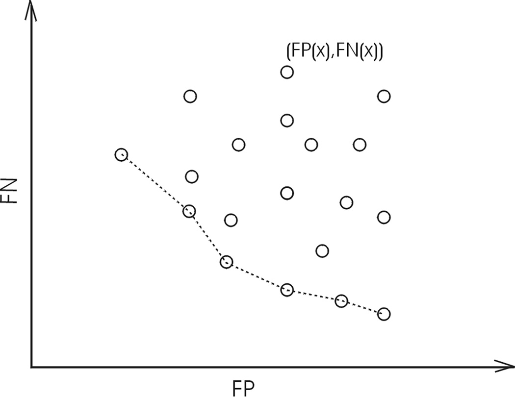
In mathematical terms, let FN and FP be described as functions of an operating parameter set x: FP(x) and FN(x), where x stands for x_A for RA and x_A+B for RA+RB. All possible performance pairs (FP(x), FN(x)) at allowed operating parameters can be mapped onto a 2D objective space (Fig. 3). A Pareto front is essentially an objective boundary such that any solution on the front can only be outperformed by another solution in at most one of the two competing objectives: lower FP or FN. Therefore, a Pareto front is also called a Pareto optimal set or a Pareto non-dominated set (Knowles and Corne, 2000).

Fig. 3.

A solution (circle) on the Pareto front (dashed line) can be outperformed by another solution in at most one of two competing objectives.

Please note that there exist two classes of approaches to find the optimal operating parameters for a multiobjective system (Messac et al. 2003). The first class involves first generating a set of Pareto solutions before selecting the optimal operating point. The second class involves forming a single objective function through some meaningful combinations of all the objective functions according to the system designer’s preference. Our approach belongs to the first class and our software implementation is discussed in the next section. Readers can refer to (Messac et al. 2003) for information of other optimization approaches.

2.4 Software Implementation

Since FN(x) and FP(x) are two conflicting objective functions with no closed form solutions, therefore, it is natural to look at this parameter setting problem as a multi-objective evolutionary problem. In this study, we used the SPEA2 (Zitzler et al., 2001) algorithm to find the Pareto set because of its fast convergence rate. The advantage of SPEA2 algorithm is discussed in more detail in (Zitzler et al., 2001) and (Li et al., 2009). In this section, we summarize our software implementation and a few key algorithmic parameters used. For more details in software implementation, readers can refer to (Li et al., 2007) and (Huang et al., 2007).

The SPEA2 algorithm was implemented in Matlab (MathWorks, Natick, Mass); region growing algorithms RA and RA+RB were first implemented and tested in C++ under Visual Studio for Windows (Microsoft, Richmond, Wash). Then fast versions of the region growing programs with the graphical part removed were recompiled in a Linux environment. To speed up computation, curvatures k₁ and k₂ at each vertex and true polyp locations were preprocessed for all 56 colon surfaces once and stored in compact, binary data files. The binary data files were then divided into multiple tasks run parallelly on a Linux Beowulf computing cluster (Bitter et al., 2004) at the National Institutes of Health (NIH).

The upper generation limits when applying SPEA2 to find the Pareto fronts for RA and RA+RB were 200 and 300 respectively. They were selected empirically. The Pareto fronts for RA and RA+RB became stable after around 150 and 250 generations respectively. A Pareto front is stable if no point on the front changes its location during one generation to the next. We found that 200 and 300 generations were adequate to approximate the asymptotic solution for the SPEA2 algorithm. They were proportional to the number of operating parameters used in x_A and x_A+B. The operating parameter ranges and conditions used in this study were: 1) H_min, H_max, H_B ∈[−10, 0) and H_min < H_max; 2) K_min ∈ [0, 50], K_max ∈ [0, 100] and K_min < K_max; 3) SI_A, SI_B∈ (0, 2]; 4) N_A, N_B ∈ [6,30]. The curvatures presented in this study were measured in cm⁻¹.

2.5 Statistical Analysis

Proper comparison of results from multi-objective optimizers is still a complex matter. Due to the random nature of the evolutionary algorithm, the obtained solutions do not always form the same Pareto front. We utilized a statistical method to compare the differences between the Pareto fronts (Section 2.3) produced by algorithms RA (Section 2.2.1) and RA+RB (Section 2.2.2) with 20 runs for each algorithm. At each FN rate, solutions from the 20 runs for both algorithms were collected into two samples. We used the two independent samples, two-tailed t test to determine whether there was a difference between the two algorithms and to estimate the 95% confidence intervals of FP reduction at each FN rate. The difference was considered significant if p-value < 0.05.

3. RESULTS

In the 20 runs, solutions for most of the possible FN rates on the Pareto fronts were found at least once for both algorithms. Exceptions were FN = 0, 84, and 86 for RA and FN = 0, 81, and 84 to 87 for RA+RB. Solutions were found at least 4 times for FN = 1 to 79 for both algorithms. Solutions were obtained 1293 and 1388 times out of 1760 (20 runs × 88 FN rates) tries for RA and RA+RB respectively. The average computation time was about 4 and 6 hours for RA and RA+RB, respectively in our parallel implementation. It was proportional to the upper generation limits 200 and 300 for RA and RA+RB respectively. (The individual execution time was roughly the same for RA and RA+RB.) The parallel implementation significantly shortened our experiment time as compared to the time of more than 30 hours needed to run on a single machine.

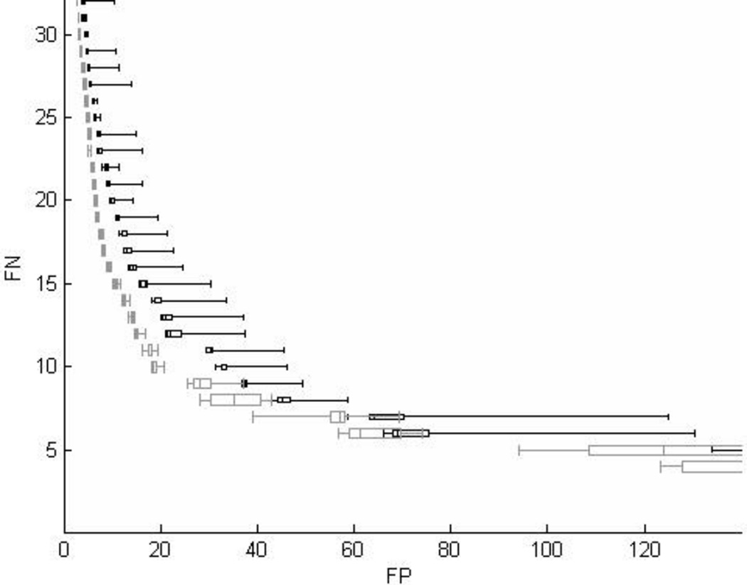
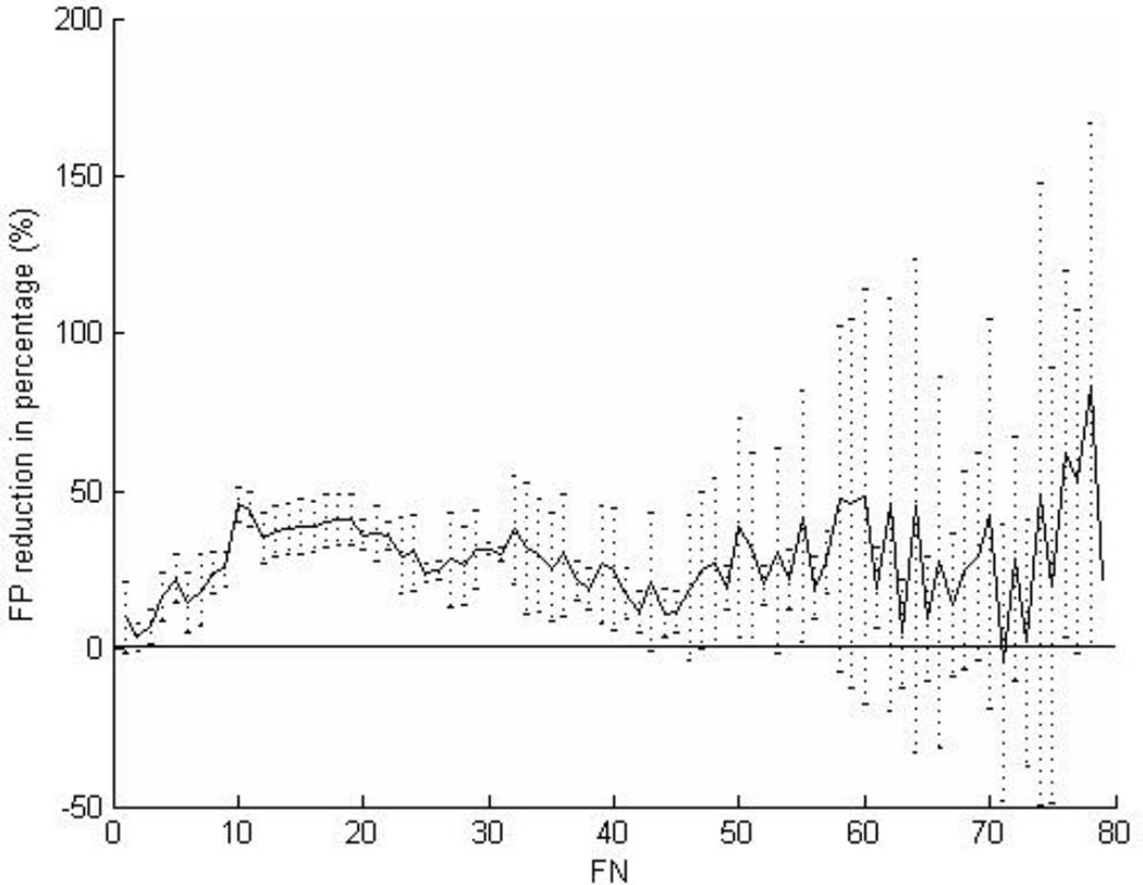
The results of the 20 runs of both methods are shown in Fig. 4. For each method, the set of solutions with the same FN rate was arranged using box-and-whisker plots (Tukey, 1977). Within each data set, solutions were arranged according to FP rates. The whiskers and box bounds from left to right were the smallest, the lower quartile, the median, the upper quartile, and the largest FP rate. By our problem definition, a better algorithm should have a lower FP rate performed at the same FN rate. In Fig. 4, the distribution of the solutions of algorithm RA+RB is clearly to the left compared with the solutions from algorithm RA. The FP reduction in percentage by RA+RB at FN = 1 to 78 is illustrated in Fig. 5. The reduction was significant (p<0.05) for 63% (55/87) of all FN rates. When operated at a suitable sensitivity level such as 90.8% (FN=8) or 88.5% (FN=10), the FP reduction rate by RA+RB with respect to RA was 24.4% (95% confidence intervals 17.9–31.0%) or 45.8% (95% confidence intervals 40.1–51.0%) respectively.

Fig. 4.

Box-and-whisker plots show the solutions from 20 runs for algorithms RA (black) and RA+RB (gray). The RA+RB shows superior performance (fewer FP at the same FN).

Fig. 5.

The FP reduction measured as difference between two means of the FP rates of RA and RA+RB divided by RA’s FP rate at FN = 1 to 78. The vertical lines illustrate the 95% confidence intervals.

Two representative solutions of the operating parameter vectors x_A and x_A+B at FN=10 are:

$${\mathbf{x}}_{\mathrm{A}}=(-10,-1.05,0.59,10.94,0.99,15)$$ (1)

and

$${\mathbf{x}}_{\mathrm{A}+\mathrm{B}}=(-10,-0.16,0,6.25,1.21,19,-1.05,0.67,11).$$ (2)

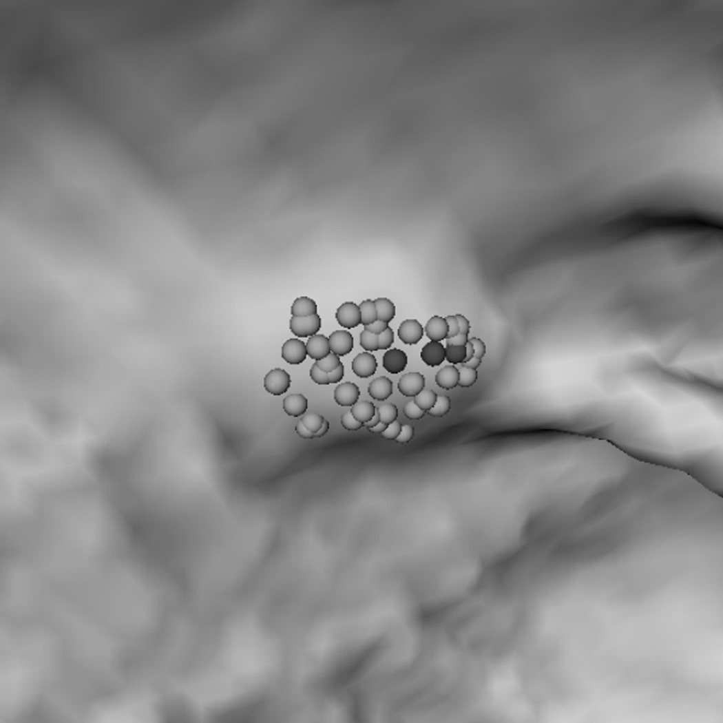
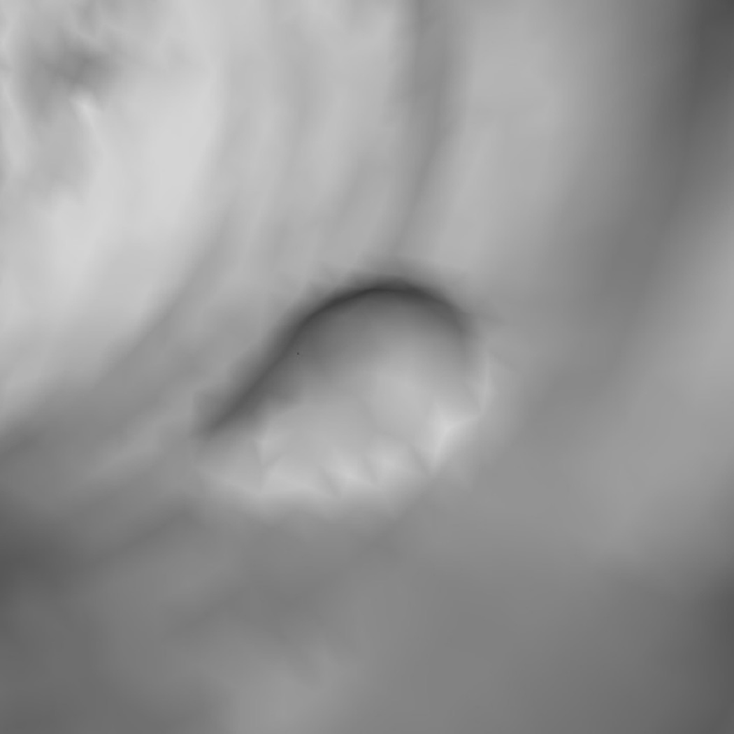
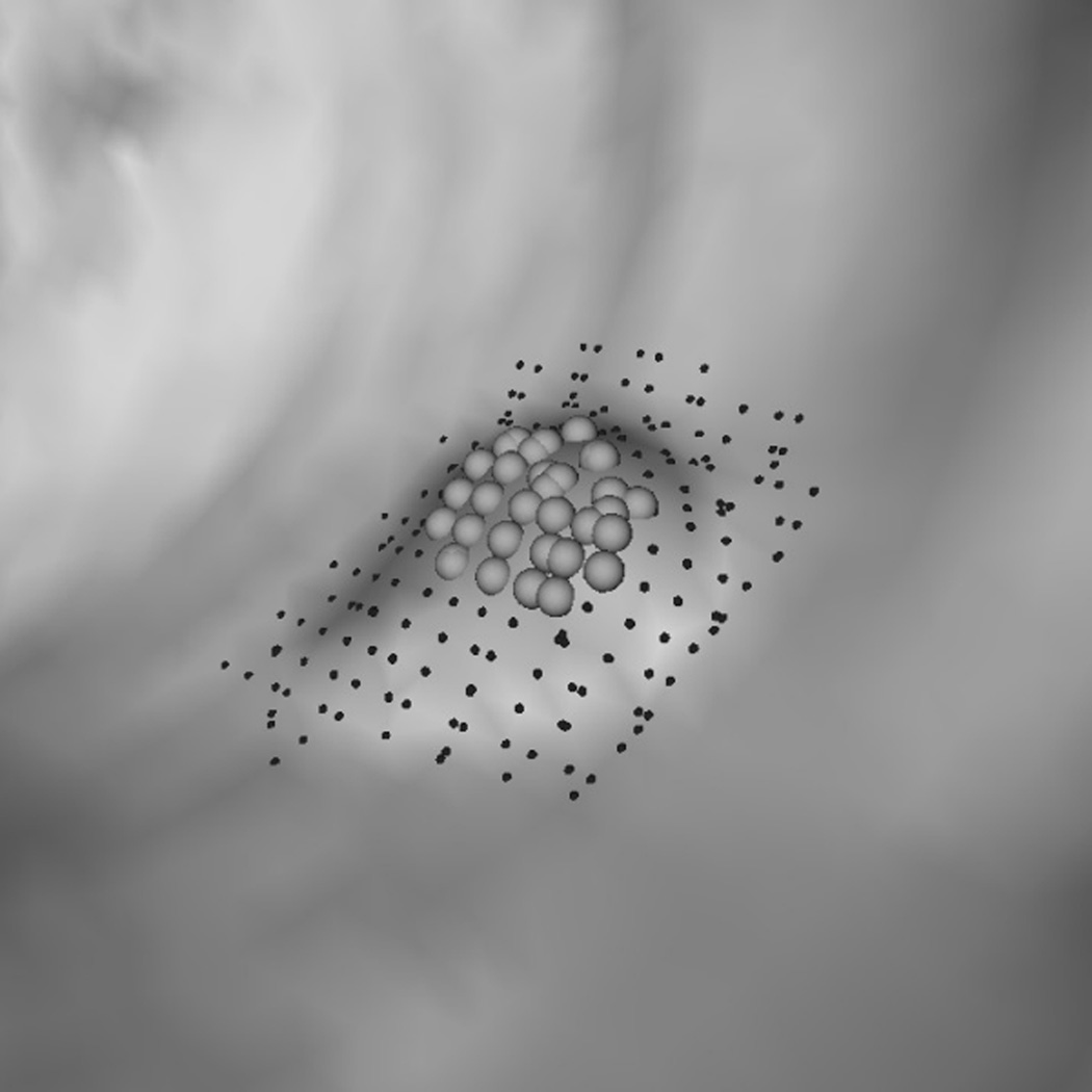
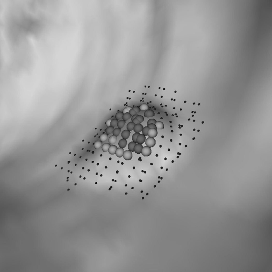
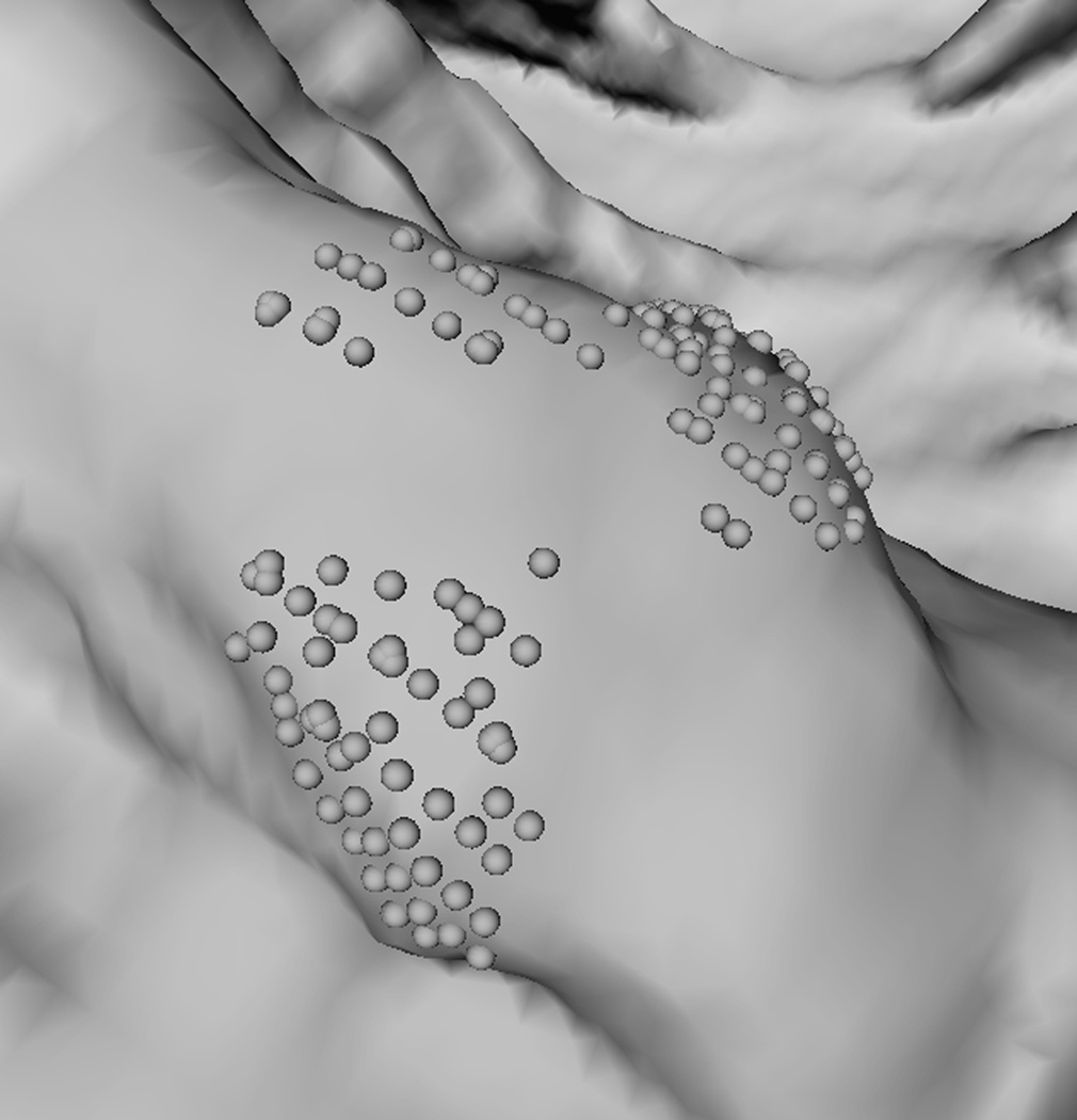
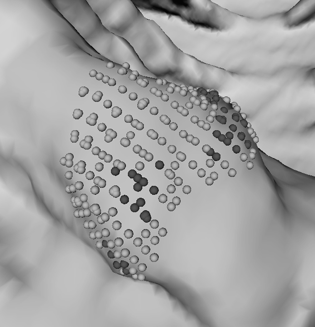
To explain why the two-step performed better, we analyzed a few polyp candidates detected by using the criteria listed above. One reason that RA+RB performs better was because it was able to distinguish a normal bump (Fig. 6a) from a 6mm adenomatous polyp (Fig. 6d). The bump had fewer polypoid vertices found by RB (Fig. 6c) and was considered less round than actual polyp candidates (Fig. 6f). Fig. 7 illustrates another observation to help explain why the two-criterion algorithm performs better. As algorithm RA used only one set of curvature criteria, the level of selectivity had to be compromising. This resulted in multiple, small detections for a large, irregular shaped polyp (Fig. 7a). On the other hand, algorithm RA+RB consisted of two sets of growing criteria. The first criterion used a lower curving condition, (H_max, K_min, K_max) = (−0.16, 0, 6.25) in (2) compared to (−1.05, 0.59, 10.94) in (1), which allowed the detection to grow into a larger cluster. The second criterion used a higher roundness condition, SI_B = 0.67 in (2) compared to SI_A = 0.99 in (1), which guaranteed that the detection had enough surface vertices resembling the shape of an ellipsoid (Fig. 7b).

Fig. 6.

(a) A polyp-like bump. (d) A 6 mm adenomatous polyp. (b, e) Resultant clusters of vertices using algorithm RA. (c, f) Resultant clusters using algorithm RA+RB. The clusters in (b, e, f) are valid candidates while (c) is not because of a small population of rounder vertices (dark gray spheres). In (c, f) light gray spheres represent vertices that satisfy a less selective criterion set (H_min, H_max, K_min, K_max) = (−10, −0.16, 0, 6.25); dark gray spheres satisfy (H_min, H_max, K_min, K_max) = (−10, −0.16, 0, 6.25) and (H_B, SI_B) = (−1.05, 0.67). In (e, f) small dots are manually marked vertices of the polyp.

Fig. 7.

A partial view of a 4 cm irregular shaped polyp. (a) Multiple detections (clusters of light gray spheres) using RA. (b) A large, single detection is formed by using RA+RB. In (b) light gray spheres satisfy a less selective criterion; dark gray spheres satisfy both selective criteria in x_A+B.

We further examined all 1388 solutions found for RA+RB from the 20 runs to identify whether or not the two-step region algorithm performed better with a less selective first step. Using the cluster population as a selectivity criterion, we found that N_A > N_B for 85% (1173/1388) of the solutions. The percentage was even higher when using the sphericity index as a selectivity criterion. We found that SI_A > SI_B for 88% (1221/1388) of the solutions where a lower SI value means rounder.

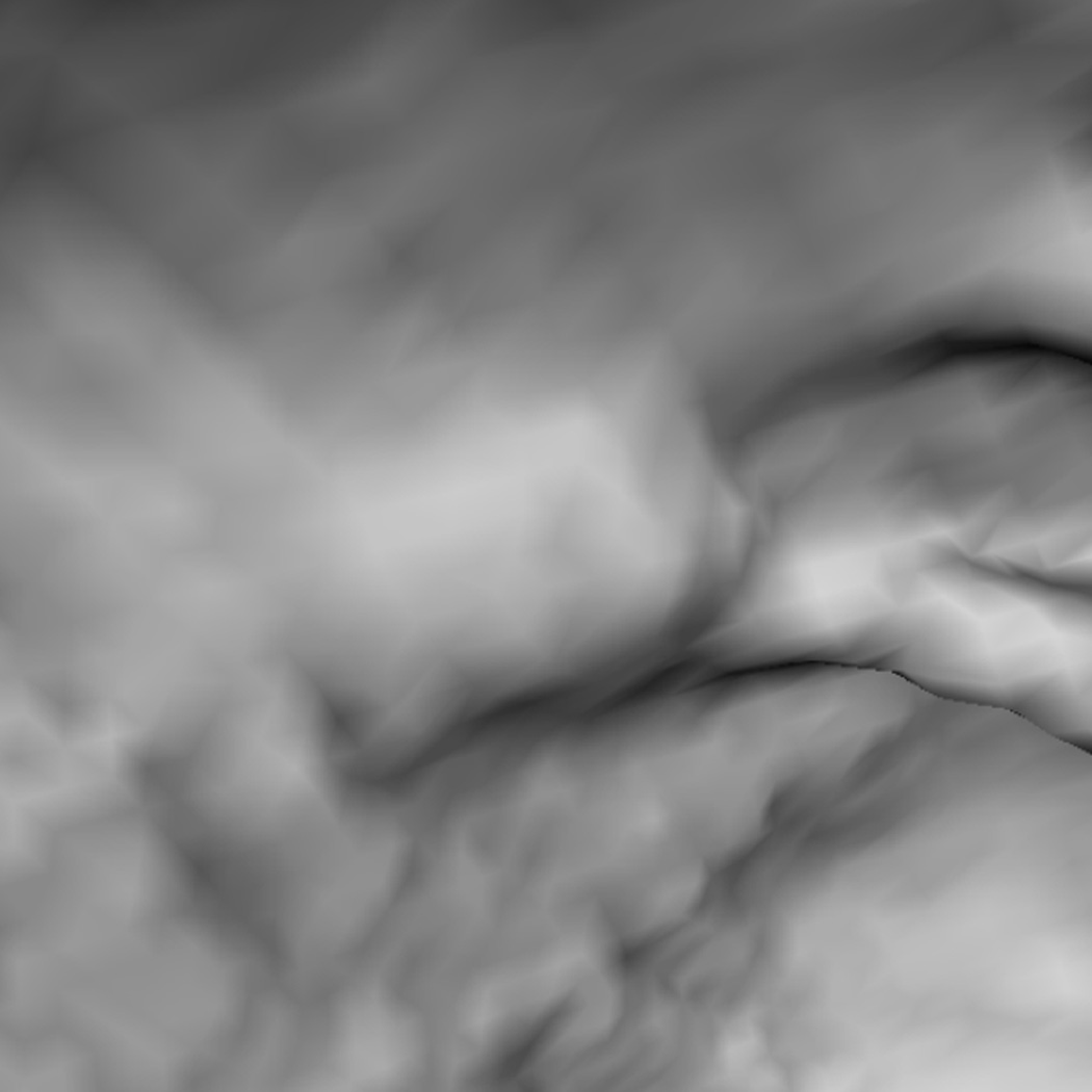
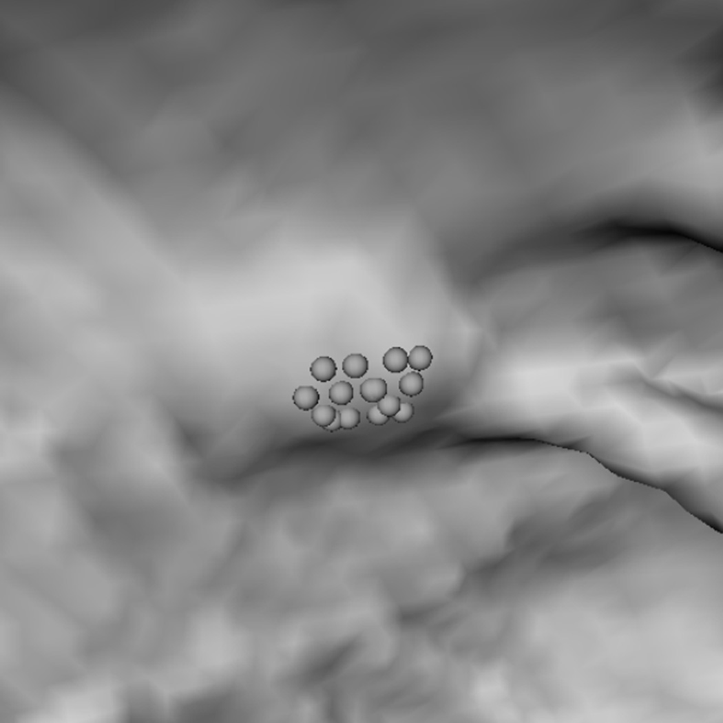
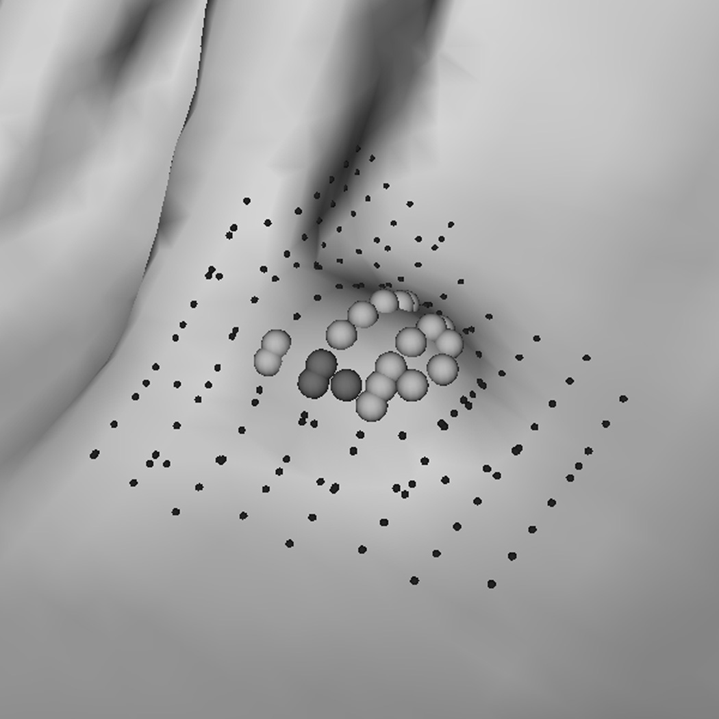
We also examined what types of polyps were more difficult to detect. At FN=10, there were three (one 3-cm and two 0.4-cm) polyps undetected on both the supine and prone surfaces and four (4-cm, 1.2-cm, 0.5-cm, and 0.4-cm) polyps undetected on either the supine or prone surface. The causes were: poor colonic distension in one case (4-cm polyp), small polyps in six cases (0.4–0.5cm polyps), and flatness/irregularity in three cases (1.2-cm and 3-cm polyps). Fig. 8 illustrates a small polyp example.

Fig. 8.

A 0.4-cm, false-negative polyp. Light gray spheres represent vertices that satisfy a less selective criterion set (H_min, H_max, K_min, K_max) = (−10, −0.16, 0, 6.25); dark gray spheres satisfy an additional, rounder criterion (H_B, SI_B) = (−1.05, 0.67); and small dots are manually marked vertices of the polyp.

4. DISCUSSION

The development of effective CTC CAD systems relies on a good evaluation and a good optimization strategy. Ideally all operating parameters of a CAD system should be optimized simultaneously. However, due to system complexity and limited computation capability, a more feasible approach is to optimize the subsystems on a component-by-component basis. Unfortunately, many image processing algorithms developed for CTC CAD systems tend to be hard to optimize by nature. Most published methods are manually adjusted to optimize sensitivity only without given enough consideration to specificity improvement. Although the performance optimization in the feature analysis stage has some merit in improving the overall CAD system, it has little value in improving polyp detection algorithms individually. In order to improve an individual CAD algorithm specifically, we must be able to evaluate the sensitivity and specificity of the subsystem simultaneously.

In this paper we investigated a Pareto front approach for evaluating and improving polyp candidate localization algorithms. Although the performance of a polyp candidate localization algorithm can be perceived as a set of paired FN and FP detection rates for all possible operating parameters, an objective performance description of an algorithm can best be characterized by the Pareto front (Fig. 3). While we can also use a summary measure such as the area under curve (AUC) to compare algorithms, it is possible for a high-AUC algorithm to perform worse in a specific region of interest for operating point selection than a low-AUC algorithm (Fawcett 2006). Therefore, the Pareto fronts are preferable because they allow us to compare polyp localization algorithms at a broader spectrum of almost all possible operating FN rates as shown in Figs. 4 and 5.

Using evolutionary algorithms to find the Pareto fronts of image processing algorithms for CTC CAD systems are somewhat computationally expensive. There are two main reasons for this. First, a typical algorithm has several adjustable and continuous operating parameters. The searching space dimensions for optimal operation are equal to the total number of these parameters. Second, colonic polyps vary in shape and size. Consequently, an adequate evaluating data set has to be large enough to cover the broad spectrum of polyp variations. Combining high parametric dimensions with large evaluating data makes finding Pareto fronts computationally expensive. For example, the region growing algorithms RA and RA+RB applied in this study only had operating parameters x_A and x_A+B of 6 and 9 variables respectively and the data set consisted of a modest size of 56 CTC surfaces, the average time to run a training session was more than 30 hours on a single machine. Fortunately, by employing a parallel implementation, the average time to run a training session was able to be shortened significantly to be within 6 hours.

Another difficulty in comparing results from multi-objective optimizers is that solutions found by evolutionary algorithms do not converge to the same solutions every time (Fig. 4). Likewise, not every solution on the Pareto front is guaranteed to be found. In order to find as many solutions as possible and achieve better approximations to the Pareto fronts of algorithms RA and RA+RB, we used a statistical approach in which each algorithm was run 20 times. In order to be able to illustrate the performance difference at every FN rate, we did not choose the statistical technique (sampling lines of intersection) used in (Knowles and Corne, 2000) and (Huang et al., 2007). Instead, we used the two independent samples, two tailed t test which allowed the estimations of 95% confidence intervals at most FN rates (Fig. 5). Note that the confidence intervals for difference in the two algorithms will only apply to this particular data set of 56 cases, and not to the population in general. To expand inference to the population in general, it requires resampling (such as bootstrapping) the 56 cases on each of the 20 runs.

Please note that our two-criterion region growing algorithm RA+RB differed from the original design proposed in (Yoshida and Nappi, 2001) in two major ways. First, the original design used a set of more selective criteria in the first step to form seed points for detecting the caps of polyps and used less selective criteria in the second step to grow the polyp bodies. Second, the original design used an extra step to merge fragmental detections. There were two main reasons to devise a new two-criterion algorithm. First, the merging step required the vertex location information. This would increase the computation time significantly because both data file loading and distance calculations were time-consuming. Second, we wanted to investigate if the polyp detection algorithm can be fine-tuned automatically by the Pareto front approach if we loosen unnecessary conditions. By removing the selectivity relations between first and second sets of criteria, we found that more than 85% of the Pareto solutions actually had a less selective first criterion set. Although no merging action was taken, the new algorithm did show some merging characteristics for large polyps (Fig. 7).

The Pareto fronts are also useful in identifying the limitation and weakness of CAD algorithms.For example, in Fig. 4 one can observe that the FP rate increases dramatically below FN=10. We examined the undetectable polyps at FN=10 and found that the main causes were size (six cases) and shape (three cases), excluding the poor distension case. Among the shape-caused FN cases, the 3-cm polyp was a flat, irregular-shaped mass that is apparent to medical doctors and can be distinguished from normal colon walls by using wall-thickening analysis (Nappi et al., 2004). However, most small and flat polyps remain a challenge because they have a modest increase in thickness and fewer polypoid-like vertices (Fig. 8).

A major limitation of our study was that we did not investigate how to select an optimal operating point from the resultant Pareto front. As the Pareto front contains many good solutions, in practice we need to select one optimal operating point based on the purpose of the CAD system on hand. Li et al. proposed an efficient, discrete approach in a recent paper (Li et al., 2009) to choose the optimal solution from a Pareto front for a CAD system. Li sampled three equally-distanced, representative points from the section of interest on the Pareto front and performed free response receiver operating characteristic curve (FROC) analysis on a whole CAD system for each sampled operating point. All of the FROC analyses were performed with a larger training data set (394 patients) and the final chosen operating point on the Pareto front corresponded to the point achieving the best FROC curve. By testing the Pareto-front-optimized CAD system on a disjoint data set of 792 patients, Li reported that the Pareto approach improved CAD performance in detecting colonic polyps 8 mm or larger by 8% from a sensitivity of 82.2% (7.0 FP per patient) to 90.6% (6.4 FP per patient).

In conclusion, the Pareto approach can give more information and confidence in evaluating the performance differences between algorithms. The computer processing time required by evolutionary algorithms can be reduced by a parallel implementation. We demonstrated that, with a proper experimental design, the Pareto optimization process can effectively help in fine-tuning and redesigning a single stage of our polyp detection algorithms. We plan to extend this optimization to the other stages of CTC-CAD algorithm to determine whether component-by-component optimization can be used to systematically improve the performance of CAD algorithms.

REFERENCES

- Anastasio MA, Kupinski MA, Nishikawa RM. Optimization and FROC analysis of rule-based detection schemes using a multiobjective approach. IEEE Trans. Med. Imag. 1998;17:1089–1093. doi: 10.1109/42.746726. [DOI] [PubMed] [Google Scholar]
- Bielen D, Kiss G. Computer-aided detection for CT colonography: update 2007. Abdominal Imaging. 2007;32:571–581. doi: 10.1007/s00261-007-9293-2. [DOI] [PubMed] [Google Scholar]
- Bitter I, Brown JE, Brickman D, et al. Large-scale validation of a computer-aided polyp detection algorithm for CT colonography using cluster computing; Proc. Med. Imag. SPIE; 2004. pp. 290–294. [Google Scholar]
- Bhotika R, Mendonca P, Sirohey SA, et al. Part-based local shape models for colon polyp detection; Proc MICCAI, LNCS; 2006. pp. 479–486. [DOI] [PubMed] [Google Scholar]
- Campadelli P, Casiraghi E, Valentini G. Support vector machines for candidate nodules classification. Neurocomputing. 2005;68:281–288. [Google Scholar]
- Campbell SR, Summers RM. Analysis of kernel method for surface curvature estimation; Proc. Med. Imag. SPIE; 2007. p. 6511. [Google Scholar]
- Chan HP, Sahiner B, Wagner RF, et al. Classifier design for computer-aided diagnosis: effects of finite sample size on the mean performance of classical and neural network classifiers. Med. Phys. 1999;26:2654–2668. doi: 10.1118/1.598805. [DOI] [PubMed] [Google Scholar]
- Chen D, Liang Z, Wax MR, et al. A novel approach to extract colon lumen from CT images for virtual colonoscopy. IEEE Trans. Med. Imag. 2000;19:1220–1226. doi: 10.1109/42.897814. [DOI] [PubMed] [Google Scholar]
- Chowdhury TA, Whelan RF, Ghita O. The use of 3D surface fitting for robust polyp detection and classification in CT colonography. Comput. Med.Imag. Graph. 2006;30:427–436. doi: 10.1016/j.compmedimag.2006.06.004. [DOI] [PubMed] [Google Scholar]
- Cotton PB, Durkalski VL, Pineau BC, et al. Computed tomographic colonography (virtual colonoscopy): a multicenter comparison with standard colonoscopy for detection of colorectal neoplasia. JAMA. 2004;291:1713–1719. doi: 10.1001/jama.291.14.1713. [DOI] [PubMed] [Google Scholar]
- Do Carmo MP. Differential Geometry of Curves and Surfaces. Englewood Cliffs, NJ: Prentice Hall; 1976. [Google Scholar]
- Fawcett T. An introduction to ROC analysis. Pattern Recognition Lett. 2006;27:861–874. [Google Scholar]
- Franaszek M, Summers RM, Pickhardt PJ, et al. Hybrid segmentation of colon filled with air and opacified fluid for CT colonography. IEEE Trans. Med. Imag. 2006;25:358–368. doi: 10.1109/TMI.2005.863836. [DOI] [PubMed] [Google Scholar]
- Frimmel H, Nappi J, Yoshida H. Centerline-based colon segmentation for CT colonography. Med. Phys. 2005;31:2665–2672. doi: 10.1118/1.1990288. [DOI] [PubMed] [Google Scholar]
- Hara AK, Johnson CD, Reed JE, et al. Detection of colorectal polyps with CT colonography: initial assessment of sensitivity and specificity. Radiology. 1997;205:59–65. doi: 10.1148/radiology.205.1.9314963. [DOI] [PubMed] [Google Scholar]
- Hong W, Qiu F, Kaufman A. A pipeline for computer aided polyp detection. IEEE Trans. Vis. Comput. Graph. 2006;12:861–868. doi: 10.1109/TVCG.2006.112. [DOI] [PubMed] [Google Scholar]
- Huang A, Summers RM, Hara AK. Surface curvature estimation for automatic colonic polyp detection; Proc. Med. Imag. SPIE; 2005. pp. 393–402. [Google Scholar]
- Huang A, Li J, Summers RM, et al. Using pareto fronts to evaluate polyp detection algorithms for CT colonography; Proc. Med. Imag. SPIE; 2007. p. 6514. [Google Scholar]
- Jerebko AK, Summers RM, Malley JD, et al. Computer-assisted detection of colonic polyps with CT colonography using neural networks and binary classification trees. Med. Phys. 2003;30:52–60. doi: 10.1118/1.1528178. [DOI] [PubMed] [Google Scholar]
- Kiss G, Drisis S, Bielen D, et al. Computer-aided detection of colonic polyps using low-dose CT acquisitions. Acad. Radiol. 2006;13:1062–1071. doi: 10.1016/j.acra.2006.05.002. [DOI] [PubMed] [Google Scholar]
- Knowles J, Corne D. Approximating the nondominated front using the pareto archived evolutionary strategy. Evolutionary Computation. 2000;8:149–172. doi: 10.1162/106365600568167. [DOI] [PubMed] [Google Scholar]
- Kodogiannis VS, Boulougoura M, Lygouras JN, et al. A neuro-fuzzy-based system for detecting abnormal patterns in wireless-capsule endoscopic images. Neurocomputing. 2007;70:704–717. [Google Scholar]
- Kupinski MA, Anastasio MA. Multiobjective genetic optimization of diagnostic classifiers with implications for generating receiver operating characteristic characteristic curves. IEEE Trans. Med. Imag. 1999;18:675–685. doi: 10.1109/42.796281. [DOI] [PubMed] [Google Scholar]
- Kupinski MA, Edwards DC, Giger ML, et al. Ideal observe approximation using bayesian classification neural networks. IEEE Trans. Med. Imag. 2001;20:886–899. doi: 10.1109/42.952727. [DOI] [PubMed] [Google Scholar]
- Li J, Yao J, Summers R, et al. An efficient feature selection algorithm for polyp detection in CAD system. International Journal on Artificial Intelligence Tools. 2006;15:893–915. [Google Scholar]
- Li J, Huang A, Petrick N, et al. Validating pareto optimal operation parameters of polyp detection algorithms for CT colonography; Proc. Med. Imag. SPIE; 2007. p. 6514. [Google Scholar]
- Li J, Huang A, Yao J, et al. Optimizing computer-aided colonic polyp detection for CT colonography by evolving the Pareto front. Med. Phys. 2009;36:201–212. doi: 10.1118/1.3040177. [DOI] [PMC free article] [PubMed] [Google Scholar]
- Mani A, Napel S, Paik DS, et al. Computed tomographic colonography feasibility of computer-aided polyp detection in a “first reader” paradigm. J. Comput. Assist. Tomogr. 2004;28:318–326. doi: 10.1097/00004728-200405000-00003. [DOI] [PubMed] [Google Scholar]
- Masutani Y, Yoshida H, MacEneaney P, et al. Automated segmentation of colonic walls for computerized detection of polyps in CT colonography. J.Comput. Assist. Tomogr. 2001;25:629–638. doi: 10.1097/00004728-200107000-00020. [DOI] [PubMed] [Google Scholar]
- Melonakos J, Mendonca P, Bhotika R, Sirohey S. A probabilistic model for haustral curvatures with applications to colon CAD; Proc. MICCAI. LNCS; 2007. pp. 420–427. [DOI] [PubMed] [Google Scholar]
- Mendonca P, Bhotika R, Zhao F, Melonakos J, Sirohey S. Detection of polyps via shape and appearance modeling; Proc. MICCAI Workshop: Computational and Visualization Challenges in the New Era of Virtual Colonoscopy; 2008. pp. 33–39. [Google Scholar]
- Messac A, Ismail-Yahaya A, Mattson CA. The normalized normal constraint method for generating the Pareto frontier. Structural and Multidisciplinary Optimization. 2003;25(2):86–98. [Google Scholar]
- Nappi J, Frimmel H, Dachman AH, Yoshida H. Computerized detection of colorectal masses in CT colonography based on fuzzy merging and wall-thickening analysis. Med. Phys. 2004;31(4):860–872. doi: 10.1118/1.1668591. [DOI] [PubMed] [Google Scholar]
- Paik DS, Beaulieu CF, Rubin GD, et al. Surface normal overlap: a computer-aided detection algorithm with application to colonic polyps and lung nodules in helical CT. IEEE Trans. Med. Imag. 2004;23:661–675. doi: 10.1109/tmi.2004.826362. [DOI] [PubMed] [Google Scholar]
- Pickhardt PJ, Choi JR, Hwang I, et al. Computed tomographic virtual colonoscopy to screen for colorectal neoplasia in asymptomatic adults. N. Engl. J. Med. 2003;349:2191–2200. doi: 10.1056/NEJMoa031618. [DOI] [PubMed] [Google Scholar]
- Rockey DC, Paulson E, Niedzwiecki D, et al. Analysis of air contrast barium enema, computed tomographic colonography, and colonoscopy: prospective comparison. Lancet. 2005;365:305–311. doi: 10.1016/S0140-6736(05)17784-8. [DOI] [PubMed] [Google Scholar]
- Sahiner B, Chan HP, Petrick N, et al. Feature selection and classifier performance in computer-aided diagnosis: the effect of finite sample size. Med. Phys. 2000;27:1509–1522. doi: 10.1118/1.599017. [DOI] [PMC free article] [PubMed] [Google Scholar]
- Summers RM, Beaulieu CF, Pusanik LM, et al. An automated polyp detector for CT colonography: feasibility study. Radiology. 2000;216:284–290. doi: 10.1148/radiology.216.1.r00jl43284. [DOI] [PubMed] [Google Scholar]
- Summers RM, Yao J, Pickhardt PJ, et al. Computed tomographic virtual colonoscopy computer-aided polyp detection in a screening population. Gastroenterology. 2005;129:1832–1844. doi: 10.1053/j.gastro.2005.08.054. [DOI] [PMC free article] [PubMed] [Google Scholar]
- Summers RM, Huang A, Yao J, et al. Assessment of polyp and mass histopathology by intravenous contrast-enhanced CT colonography. Acad. Radiol. 2006;13:1490–1495. doi: 10.1016/j.acra.2006.09.051. [DOI] [PubMed] [Google Scholar]
- Tukey JW. Box-and-Whisker plots, in: Explanatory Data Analysis. Reading, Mass: Addison-Wesley; 1977. pp. 39–43. [Google Scholar]
- Van Wijk C, van Ravesteijn VF, Vos FM, et al. Detection of protrusions in curved folded surfaces applied to automated polyp detection in CT colonography; Proc. MICCAI, LNCS; 2006. pp. 471–478. [DOI] [PubMed] [Google Scholar]
- Wagner RF, Chan HP, Mossoba JT, et al. Finite-sample effects and resampling plans: applications to linear classifier in computer-aided diagnosis; Proc. Med. Imag. SPIE; 1997. pp. 467–477. [Google Scholar]
- Winawer SJ, Zauber AG, Ho MN, et al. Prevention of colorectal cancer by colonoscopic polypectomy, the National Polyp Study Workgroup. N. Engl. J. Med. 1993;329:1977–1981. doi: 10.1056/NEJM199312303292701. [DOI] [PubMed] [Google Scholar]
- Yao J, Miller M, Franaszek M, et al. Colonic polyp segmentation in CT colonography-based on fuzzy clustering and deformable models. IEEE Trans. Med. Imag. 2004;23:1344–1352. doi: 10.1109/TMI.2004.826941. [DOI] [PubMed] [Google Scholar]
- Yao J, Summers RM, Hara AK. Optimizing the committee of support vector machines (SVM) in a colonic polyp CAD system; Proc. Med. Imag. SPIE; 2005. pp. 384–392. [Google Scholar]
- Yee J, Akerkar GA, Hung RK, et al. Colorectal neoplasia: performance characteristics of CT colonography for detection in 300 patients. Radiology. 2001;219:685–692. doi: 10.1148/radiology.219.3.r01jn40685. [DOI] [PubMed] [Google Scholar]
- Yoshida H, Nappi J. Three-dimensional computer-aided diagnosis scheme for detection of colonic polyps. IEEE Trans. Med. Imag. 2001;20:1261–1274. doi: 10.1109/42.974921. [DOI] [PubMed] [Google Scholar]
- Yoshida H, Dachman AH. CAD techniques, challenges, and controversies in computed tomographic colonography. Abdominal Imaging. 2005;30:26–41. doi: 10.1007/s00261-004-0244-x. [DOI] [PubMed] [Google Scholar]
- Zitzler E, Laumanns M, Thiele L. [Accessed August 2, 2007];Spea2: Improving the Strength ParetoEevolutionary Algorithm, Swiss Federal Institute of Technology, Technical Report TIK-Report 103, 2001. 2001 Available at: http://e-collection.ethbib.ethz.ch/ecol-pool/incoll/incoll_324.pdf.