Model-based Blind Estimation of Kinetic Parameters in DCE-MRI

Abstract

A method to simultaneously estimate the arterial input function (AIF) and pharmacokinetic model parameters from dynamic contrast-enhanced MRI data was developed. This algorithm uses a parameterized functional form to model the AIF and k-means clustering to classify tissue time-concentration measurements into a set of characteristic curves. An iterative blind estimation algorithm alternately estimated parameters for the input function and the pharmacokinetic model. Computer simulations were used to investigate the algorithm's sensitivity to noise and initial estimates. In 12 patients with sarcomas, pharmacokinetic parameter estimates were compared with “truth” obtained from model regression using a measured AIF. When arterial voxels were included in the blind estimation algorithm, the resulting AIF was similar to the measured input function. The “true” K^trans values in tumor regions were not significantly different than the estimated values, .99±.41 and .86±.40 min⁻¹ respectively, p=0.27. “True” k_ep values also matched closely, .70±.24 and .65±.25 min⁻¹, p=0.08. When only tissue curves free of significant vascular contribution are used (v_p<0.05), the resulting AIF showed substantial delay and dispersion consistent with a more local AIF such as has been observed in dynamic susceptibility contrast imaging in the brain.

Introduction

Dynamic contrast enhanced (DCE)–MRI is a non-invasive, physiological imaging tool that involves the repeated acquisition of images of a particular region of interest (ROI). During the image acquisition, a contrast agent (CA) is administered intravenously, normally by bolus injection. The relaxation rate of tissues within the ROI is affected by the concentration of CA, the time course of which can be related to physiologically-interesting parameters including vascular permeability-surface area product (K^trans), contrast washout rate (k_ep), blood plasma volume fraction (v_p), and extracellular volume fraction (v_e). Accurate quantitative estimation of these parameters provides important information on underlying tissue physiology (1).

Pharmacokinetic model parameters can be estimated from DCE-MRI data by fitting a pharmacokinetic model to measured CA curves using either ROI-averaged or single voxel data. Numerical solution of these models generally requires a priori knowledge of the blood pool CA concentration, commonly known as the arterial input function (AIF). Direct measurement of the AIF is possible via physical blood sampling, but this approach has poor temporal resolution and is complex and time-consuming, making it impractical for use in routine clinical imaging. Determination of the AIF directly from the DCE-MRI data is also possible, but requires a suitable artery in the imaging field of view (FOV). In some imaging situations, no such artery is present in proximity to the tissue ROI, necessitating the use of a larger FOV than would be otherwise necessary to encompass the tissue of interest, with concomitant decrease in resolution and/or increase in imaging time. In other situations the arterial lumen is small relative to the imaging voxel size, leading to systematic underestimation of the AIF due to partial volume effects. Signal saturation effects may lead to underestimation of the peak concentration. Insufficiently rapid temporal sampling also leads to underestimation of peak concentration. Furthermore, noise in measured AIFs can lead to large variation in pharmacokinetic parameter estimates due to the sensitivity of the deconvolution process (2,3). For these reasons, the ability to determine the AIF and model parameters simultaneously from measured tissue data is a desirable goal.

A number of methods have been proposed as alternatives to direct measurement of the AIF. Use of a population-averaged AIF (4) has the advantage of simplicity but is unable to account for variation in the AIF from scan to scan or patient to patient. Yankeelov et al. and Yang et al. have explored the use of reference region approaches, comparing measured data in healthy tissue to literature values and thus extracting the AIF (5-8). Yang et al. have also incorporated reference values with indirect measurement approaches (6). While these methods have shown some promise, they require a priori assumptions about the values of model parameters in “normal” tissues. Such approaches are limited by variability in these normal tissues and by the need to incorporate a significant region of a well-characterized normal tissue within the FOV.

This work focuses on blind estimation techniques for extracting kinetic parameters and AIFs simultaneously from DCE-MRI data that do not require either measured AIF data or statistical estimates of pharmacokinetic parameters in reference tissues. We build on the work reported previously by Riabkov and DiBella (9) that used the iterative quadratic maximum likelihood (IQML) algorithm for blind estimation of kinetic parameters, and also on a similar approach by Yang et al (6). A key difference here is firstly that a novel functional form for the input function, which can accurately model the shape of the AIF while simultaneously minimizing the effect of noise, is introduced. A second important difference in this work is that the characteristics of AIFs that are estimated when arterial voxels are not included in the field of view are studied. That is, blind estimation using time curves from both tissue and arterial voxels provides input functions similar to those measured directly from the arterial voxels. In contrast, when arterial voxels are excluded from the estimation process, with the algorithm based on only tissue curves from a particular region, the resulting input function is dispersed and delayed as compared to the AIF measured in the arterial voxels. This suggests that the “true” input function seen by tissue voxels is different from that measured in a nearby artery, consistent with the work of Calamante and others on local input functions measured using dynamic susceptibility contrast in the brain (10,11). We discuss the mathematical basis of our algorithm and present preliminary results on both simulated and measured data.

Methods and Materials

Blind Estimation Analysis

The basic algorithm used here is described in detail in (9). We begin with an extended Tofts-Kety two compartment model for tissue CA concentration:

$$C_t\left(t\right)=K^{\mathit{trans}}{C}_p\left(t\right)\otimes e^{-k_{\mathit{ep}}t}+V_p{C}_p\left(t\right)$$ (1)

where K^trans and k_ep are the transfer constant and rate constant respectively, ⊗ is the convolution operator, v_p is the blood plasma volume fraction, and C_p(t) is the concentration of CA in the blood plasma (1). The blind estimation method takes advantage of the discrete nature of MRI data and creates an objective function:

$$R=\Vert \overrightarrow{C_t\left(\mathit{t}\right)}-[\mathit{H}+\Delta ]\overrightarrow{C_p\left(t\right)}\Vert$$ (2)

where H denotes the convolution matrix and Δ denotes a diagonal matrix representing v_p. C_t(t) is a matrix consisting of the tissue concentration curves input to the algorithm. This function (Eq. 2) is minimized by alternately varying the kinetic parameters and the AIF. A population-averaged input function, which has been shown to yield reasonable estimates for kinetic parameters (12), is used as the initial guess for the AIF. The initial guesses for pharmacokinetic parameter values are estimated via a non-linear least-squares algorithm using this initial guess for the AIF. The pharmacokinetic parameter values are then held fixed and a new AIF estimate is computed by the same least-squares algorithm. This alternating optimization continues until the regression has converged to an AIF. In our implementation the MATLAB lsqcurvefit function was used to perform the nonlinear regressions. Default convergence criteria were used, and parameter values were bounded to prevent non-physiological negative values.

We use a model parameterization of the following form to represent the AIF (13):

$$C_p\left(t\right)=\underset{i=1..2}{\Sigma }{A}_i{\gamma }_v\left({\alpha }_i,{\tau }_i\right)+A_{3}S({\alpha }_3,{\tau }_3,T,\Delta )$$ (3)

which consists of two normalized gamma-variate curves (γ_i) representing the first and second passes of the CA bolus, and a normalized sigmoid function (S) representing the decaying washout of CA from the ROI. This function is fully described with 11 parameters, and can model a wide range of physiological input functions, similar to that developed by Parker et al (4). By choosing a flexible analytic form for the AIF, we minimize the impact of AIF measurement noise, which otherwise could be amplified at each step of the minimization process. At each iteration of the alternating minimization with model (AMM) algorithm, the new AIF estimate is constrained to this functional form by nonlinear regression using a least-squares approach.

We also changed the implementation of the minimization process from that in (9) to include a delay time between the arrival of the CA bolus in the arterial blood and in the tissue of interest. During each iteration, when fitting the tissue curves to the AIF, the AIF was allowed to shift in time to obtain a best fit.

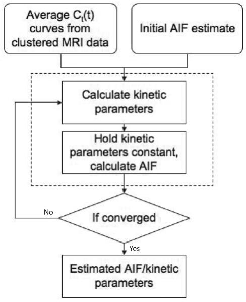
As reported in (9), the IQML algorithm can only estimate K^trans to within a global scaling constant. To constrain this scale factor, at the end of each iteration the average value of the last five values of the estimated AIF is normalized to the average of the last five time points of the AIF obtained from a nearby region of arterial voxels. At the beginning of the next iteration the estimated AIF is adjusted so that the average concentration of the tail of the estimated AIF matches that of the measured arterial voxels. In practice, it is assumed that following the imaging of the FOV of interest a few images of a nearby artery would be acquired. This acquisition could be optimized for concentration measurements of the equilibrium blood pool concentration. The lower CA concentration several minutes after injection would be less susceptible to non-linear saturation effects. In addition, moving the imaging field of view to a larger artery would lessen the impact of partial volume effects, allowing for a better estimate for the scaling constant for the estimated AIF. This AIF can then be used with any conventional deconvolution or curve-fitting methods to determine kinetic parameters for any pixel in the FOV. The sequence of steps leading to the determination of the AIF is summarized in Fig. 1.

Fig. 1.

Flow chart for the AMM method. This method requires several tissue concentration curves and some estimate for the AIF as input. The algorithm will alternately calculate the kinetic parameters for each input concentration curve and the common input function.

Sensitivity to Initial Estimate of AIF Parameters

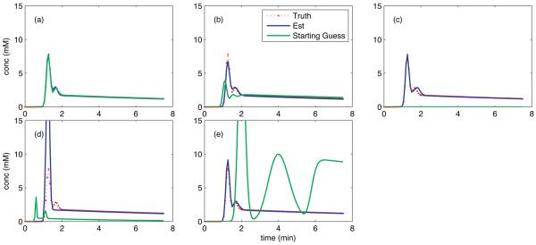
The AMM method uses a population-averaged input function as a starting guess. To test the sensitivity of the algorithm to this initial guess for the AIF, we generated simulated tissue concentration curves using a model AIF generated using Eq. 3 with the following parameter values: A₁=7.8, α₁=1.26, τ₁=0.00663, A₂=1.2, α₂=1.65, τ₂=0.00555, A₃=1.9, α₃=44, τ₃=0.018, Δ=0.7, and T=15. Both the AIF and tissue curves were discretized at 4.5 second temporal resolution and truncated after 7.5 min. The resulting AIF is shown in Fig. 2. Ten sets of four tissue curves were created from the ‘true’ AIF with pharmacokinetic parameters drawn from a uniform random distribution. K^trans was constrained to [0,2.2] min⁻¹, v_e to [0.15,1], and v_p to [0,0.2]. Zero mean Gaussian noise with a standard deviation of 0.08 mM, corresponding to an average SNR of 8 was added to the simulated tissue curves and each set of four curves were input to the AMM method for each of five different initial guesses for the AIF.

Fig. 2.

Estimated AIFs resulting from variations in initial guess to the AMM method (blue). The initial guess used (green) were truth (a), near truth (b), zero (c), and the lower (d), and upper (e) bounds on the constraints used in the estimation algorithm. For comparison, truth has been plotted on each panel (red). All graphs have the same temporal resolution, shown in red.

The five initial guesses supplied to the AMM algorithm were: the ‘true’ AIF, a slightly modified version of the ‘true’ AIF with parameters: A₁=4, α₁=1.1, τ₁=0.009, A₂=1.5, α₂=1.5, τ₂=0.01, A₃=2, α₃=40, τ₃=0.03, Δ=0.5, and T=20, a zero-valued vector, and the lower and upper bounded AIF from the minimization process, with parameters: A₁=1, α₁=0.5, τ₁=0.002, A₂=0.25, α₂=0.5, τ₂=0.002, A₃=0.25, α₃=5, τ₃=0.001, Δ=0.5, and T=5 and: A₁=30, α₁=2, τ₁=0.01, A₂=10, α₂=4, τ₂=0.03, A₃=10, α₃=60, τ₃=0.05, Δ=4, and T=30 respectively.

The process was repeated for each initial guess with each set of four randomly generated tissue curves. Estimates for the pharmacokinetic parameters for each of the four input curves were calculated. The relative error of these estimates was computed as a measure of the error introduced by the variation in initial guess.

Noise Sensitivity Simulation

Kinetic parameter estimates from the AMM algorithm were compared to parameter estimates from a measured AIF with a noise simulation based on patient data. A portion of a single slice of patient data with a significant amount of diseased tissue was selected. The measured AIF from this scan was then fit to the model in Eq. 3, and this AIF was used to estimate kinetic parameters for the region. The AIF and estimated parameters were then treated as truth and noise free tissue curves were created according to Eq 1 with temporal resolution of 4.5 seconds/frame. Four sets of kinetic parameters were randomly generated within bounds set to match those from the patient data and zero-mean Gaussian noise with standard deviations of 0.02, 0.04, 0.08, and 0.16 mM was added to the tissue curves. For reference, the average standard deviation in the background noise in the original measured data was 0.08 mM, which corresponds to an SNR on the order of 8.

For conventional (non-blind) estimation of the kinetic parameters from the simulated data, noise corresponding to the level added to the tissue curves was added to the simulated AIF, scaled by the square root of 19, which was the number of pixels used to calculate the AIF in the original dataset. The AIF was shifted by a random fraction of the sampling time to simulate jitter. The jittered AIF was then used to calculate the kinetic parameters.

For the blind estimation method, the kinetic parameters were estimated using the AMM algorithm. In addition, the blind estimation algorithm was implemented at each noise level without including any analytic form for the input function. 100 noise realizations were used at each noise level, with four new tissue curves generated randomly at each realization. The ‘conventional’ AIF was jittered during each realization. The resultant kinetic parameters from the simulated measured AIF, the AMM method and the alternating minimization without model were then compared with truth, and the relative error was computed.

The noise sensitivity simulation was repeated with a second set of patient data. This set was selected for having the AIF that was the most widely dispersed in time over all of the patient data used in this paper. The simulation methodology was identical to that used with the first patient AIF.

Patient Data

The blind estimation algorithm was applied to DCE-MRI data from 12 patients diagnosed with various soft-tissue sarcomas. Data was acquired on a Siemens 1.5T scanner using a FLASH 3D sequence with 20° flip angle, and TR ranging from 2.81-3.59 ms and TE ranging from 1.13-1.44 ms. 20mL of Omniscan was administered intravenously with a dose of 0.1-0.2 mmol/kg of body weight. The temporal resolution of the scans ranged from 3.5-4.9 seconds/frame. 12-18 slices were obtained from each scan, with 96-512 voxels acquired along the frequency and 128-512 voxels along the phase-encode axei. All data was obtained with written consent and was IRB approved. Measured DCE-MRI images were converted into CA concentration by solving the nonlinear relationship between the FLASH signal and CA concentration, as described in (13). Pre-contrast T10 values were determined using a variable flip angle method (14). This non-linear conversion technique minimizes the impact of underestimation of true contrast concentration due to signal saturation at high CA concentrations.

Each dataset contained arterial voxels from which a measured AIF was extracted. The AIF used was selected from the voxels with the highest overall concentration values and earliest uptake times. The AIF selection was done automatically, similar to the method described in (15). This measured AIF functioned as ‘truth’ in comparison with the blind-estimation-extracted AIF. Due to the large size of the patient data sets a portion of single slice through the lesion of interest was selected from each patient for analysis, with the portions averaging 250 × 250 voxels. Each slice was selected so that it also contained arterial voxels, as determined by the AIF measurement technique described above, and the blind estimation algorithm was applied twice. During the second run, any arterial voxels in the selected slice were excluded from use in the blind estimation. The arterial voxels were selected for exclusion based on their shape, specifically the ratio of the height of the first pass of the CA bolus to the average concentration over the rest of the curve. This was done to test the assumption that AMM may be used in situations where no artery exists within the imaged FOV, or when the clinician may wish to limit the FOV to the region immediately surrounding the area of interest. In both cases, the automatically-extracted AIF was used to scale the estimated AIF as described above.

In order to determine the set of curves, here called C_t(t) or tissue concentration curves, to be input into the alternating minimization, the data are clustered into groups of similar curves using an unsupervised k-means algorithm. The number of clusters is determined empirically with the goal that each cluster has a minimum of intra-cluster variability, here defined as the average of the within-cluster sums of point to centroid differences, measured as the vector sum of the Euclidian norms. The tissue concentration curves within each cluster are averaged to obtain a representative curve from every cluster. These cluster-averaged curves are then used in the implementation of the blind estimation algorithm.

After CA concentration curves have been obtained from the MRI data they are clustered into groups of similar curves with k-means clustering as described above. The total number of clusters selected is limited by the number of voxels in the dataset under investigation. Smaller datasets yield clusters with fewer tissue concentration curves per cluster. These small clusters produce average curves with lower SNR than would result when opting to use less clusters. With patient data, the algorithm returned nearly identical values for the pharmacokinetic parameters over a range of four to ten clusters in each dataset. In most instances, eight clusters seemed adequate from empirical testing and eight clusters were used throughout for the patient data.

After an estimated input function has been obtained from the AMM method, kinetic parameter estimates were obtained voxel-wise via a linearized least-squares approach outlined in (17). This approach was selected for its increased speed with respect to non-linear approaches.

Results

Sensitivity to Initial Estimate of AIF Parameters

Mean estimated AIFs from each of the five initial guesses are shown in Fig. 2. When the initial guess for the AIF matches truth, the algorithm converges rapidly (often in a single iteration) (panel a). When the initial guess is close to truth (b) or uniformly zero (c), the resulting AIF results in kinetic parameters estimates with a median relative error of 8%. Panel (d) represents the lower bound on the 11 AIF parameters in the AMM process. This very poor initial guess for the AIF results in a 300% over-estimation of the peak value of the AIF, with a corresponding 65% median relative error in the kinetic parameters. Panel (e) represents another intentionally poor initial estimate, the upper bound on the 11 AIF parameters, and results in an AIF yielding 15% median relative error in the kinetic parameters.

Noise Sensitivity Simulation

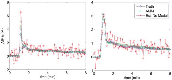
As stated above, the sensitivity of the algorithm to noise was determined by adding Gaussian noise to a set of tissue curves before applying the blind estimation process. The accuracy of the algorithm was determined by the relative error of the fit kinetic parameters. As shown in Fig. 3, the average error in K^trans and k_ep estimates is 5% higher for the AMM method as compared to the more conventional, measured AIF method. The minimization without model results for K^trans have the same error as the AMM method at noise levels of 0.04 mM and smaller, but as noise increases, the relative error increases to a maximum of 36%, with the AMM maximum at 22%. The estimates for k_ep are not as good when the AIF model was not used, with an average of 13% higher relative error as compared to AMM. v_p measurements were highly sensitive to small variations in the estimated input function. In addition, v_p measurements tend to be on the order of 0.10, and thus small changes in the estimates yield high percent errors. All of the analysis methods had some error at a zero noise level. This error is due to the coarse temporal resolution used in these simulations. When the temporal resolution was increased to 0.5 s per time sample, all the estimation techniques returned zero error when no noise was added to the simulated curves. Representative results from a single noise realization at a noise level of 0.08 mM are shown in Fig 4 for both of the test AIFs.

Fig. 3.

The relative error in estimated kinetic parameters after noise has been added to simulated tissue concentration curves. The error in the kinetic parameters was less when the functional model for the AIF was included in the alternating minimization (black), as compared to when no restrictions were placed on the input function (red) and is 10% higher than the error from measurements using a conventionally acquired AIF (blue). The χ² fits of the estimated input functions are also shown.

Fig. 4.

AIFs used in noise sensitivity simulation (blue). Representative estimated AIFs from the AMM method when the model was included (green) and not included (red) are also shown.

Patient Data

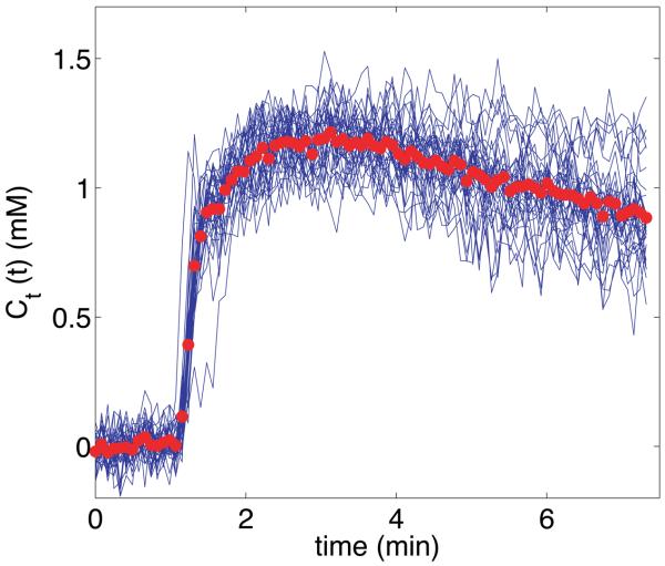
Fig. 5 shows the tissue concentration curves from one representative cluster along with the average cluster value used in the AMM process. Averaging the curves in each cluster served to reduce the noise in the data and provided a representative value for the curves in the cluster.

Fig. 5.

Representative tissue concentration curve cluster from a sarcoma patient. The blue curves represent single-voxel activity from the tumor rim. The bold red circles indicate the average value of all curves in this cluster, and were used as an input to the AMM algorithm.

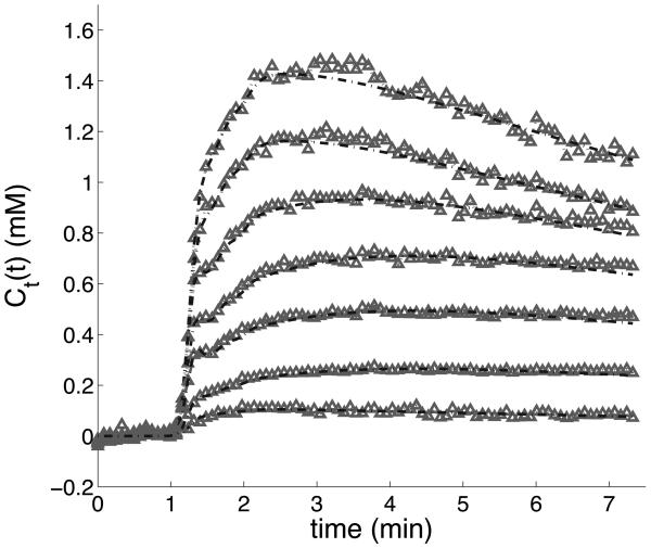
Fig. 6 shows results from the AMM process for a patient. The fitted curves closely match the measured data during the initial arrival of CA to the tissue. Overall curve fitting has similar χ² values to that done with arterially measured AIFs.

Fig. 6.

Curve-fitting results from the AMM algorithm with eight clusters used as the input. The gray points represent the average-valued curves from each cluster. The dashed-line functions were constructed from the estimated kinetic parameters and AIF from the AMM algorithm, according to the two compartment model. The eighth cluster contained only background noise and has been deleted.

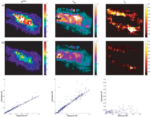
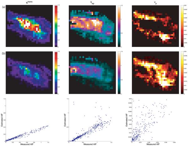
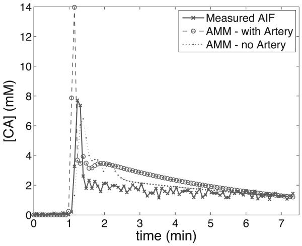
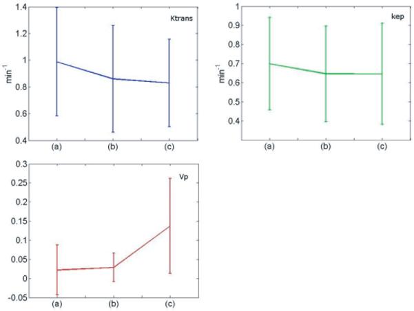
Representative maps of kinetic parameters from the same patient are shown in Figs. 7 and 8. Kinetic parameters were obtained by the method described in (16), using the measured AIF from the DCE-MRI data (first row), and those computed by the AMM method (second row). The AIFs from the AMM method in Fig. 7 were estimated when arterial voxels were included in clustering. The parameters obtained from the estimated AIF are lower than those from the measured AIF due to the increased peak height in the estimated AIF over the measured AIF. In Fig. 8 arterial voxels were not included in the estimation process. The K^trans and k_ep values obtained from the estimated AIF are lower than those from the measured AIF, though the v_p values are higher. Fig.9 shows the measured AIF from this patient's data. In addition the tissue AIFs resulting from the AMM method with and without the inclusion of arterial voxels are overlaid for easy comparison. For each of the twelve datasets, three ROIs were drawn and used to calculate average kinetic parameters. Two ROIs were selected from a region of diseased tissue, the other from a region of healthy tissue. The average values of the kinetic parameters for these regions are summarized in Fig. 11. The average K^trans values resulting from the measured AIF are 13% higher than those from the AMM-derived AIFs with arterial voxels and 16% higher than those from AMM when arterial voxels were excluded. The average k_ep values obtained from the measured AIFs were 7.5% higher than those from the AMM method with or without arterial voxels. The measured AIF and arterial voxel AMM average values for v_p differ by less than 0.007 while those resulting from AMM without arterial voxels are approximately 0.1 higher. A two-tailed dependent student's t-test showed that the differences in parameters were not significant (P>0.5) with the exception of the differences in v_p estimated with the measured AIF and the estimated AIF when arterial voxels were excluded (P=0.0005).

Fig. 7.

Parameter mapping results. The first row (a) used the measured AIF. The second row (b) was derived from the estimated AIF using arterial voxels. The third row shows scatter plots of the parameters displayed in row (a) (x-axis) and row (b) (y-axis). The patient was scanned near the distal humerus, with the AIF measured in the brachial artery. The region shown is from a neurofibroma.

Fig. 8.

Parameter mapping results. The first row (a) used the measured AIF. The second row (b) was derived from the AIF estimated when arterial voxels were excluded. The third row shows scatter plots of the parameters displayed in row (a) (x-axis) and row (b) (y-axis). These maps correspond to the same region as in Fig. 7.

Fig. 9.

AIFs from the patient data seen in Figs. 7&8. The measured AIF was obtained through an automated process similar to that described in (15), and the tissue AIFs are the result of the AMM algorithm when arterial voxels were included and excluded.

Fig. 11.

Relative mean changes for each of the pharmacokinetic parameters and standard deviation of each measurement. The parameters were measured from 12 patients, with two ROIs selected from each patient. Each chart shows the parameter value when derived from the measured AIF (a), the estimated AIF when arterial voxels are included (b), and the estimated AIF when arterial voxels are excluded (c).

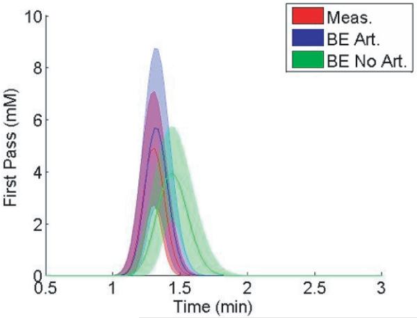
The differences in kinetic parameters result from the different shape in the resulting AIFs from the AMM method when arterial voxels are included and excluded in the estimation. Fig. 12 shows the mean and standard deviation of the AIFs from the patient data, one of which included arterial voxels, and one resulting from the exclusion of that data. The distinctly different heights and widths of the estimated AIF during the first pass of the bolus suggest that the inclusion of arterial voxels impacts the estimated AIF.

Fig. 12.

Average performance of the AMM algorithm for twelve patients. The curves represent the mean (center) and standard deviation of the first pass bolus of the AIF derived from measured voxels (red), or from the AMM method when arterial voxels are included (blue) and excluded (green). The first gamma-variate curve from the AMM model was used to describe the first pass.

Discussion

Here we have presented a method for estimating pharmacokinetic parameters from DCE-MRI data without explicitly measuring the AIF. Reference region methods for determining kinetic parameters without a measured AIF have been proposed (5,7,17,18). However, these methods require the use of one or more reference regions for which assumed values for the kinetic parameters for these reference regions must be provided. While the reference region approach appears fairly robust in dealing with low SNR data and has been shown to give results similar to those derived from a known AIF, the assumptions inherent in this class of methods may lead to unnecessary bias in the resulting kinetic parameters. For instance, though literature values for kinetic parameters in reference regions may be generally accurate, they do not allow for inter-patient individuality and thus introduce some bias into the results.

A method similar to the one described here has been proposed by Yang et al. (5,6) that makes use of multiple tissue concentration regions used jointly to identify kinetic parameters and an AIF simultaneously. This method imposes a local polynomial smoothing to ensure a smooth form for the AIF curve. In addition, one region used in this method is assumed to be skeletal muscle in which the v_p term is forced to be close to, or equal to zero. As well, v_e is set to 0.12 in the skeletal muscle region in their model. This is done to provide a reference for the general scale factor needed to quantify estimated parameters. This method performed well on real data when one concentration region contained a high percentage of pixels with arterial blood, but was only demonstrated on a single patient (6).

The AMM method presented here uses tissue concentration curves from a portion of the image and blindly estimates the input function through an iterative algorithm. The basic assumptions in this method are common to the extended Tofts-Kety two compartment model: tissues may be represented as separate compartments in and out of which contrast agent is free to diffuse. Additionally, the CA is assumed to be well mixed within the blood pool in the fast-exchange limit. The AMM method is unique in assuming a novel functional form for the input function as defined in Eq. 3. Analytical forms for the input function in dynamic imaging have been proposed with Gaussian (4) and exponential or multi-exponential (19,20) curves. The particular form chosen here was selected for its flexibility and quality of fit across multiple datasets. For blind estimation, constraining the input function to a particular functional form ensures smoothness and increases the efficiency of the algorithm by limiting the number of unknown variables. When the input function was allowed to vary without any constraints in the algorithm, the resulting AIF was significantly noisier than the tissue curves. The simulations also showed that kinetic parameter measurements are more accurate at higher levels of noise when the input function model is included. This suggests that the model constraint helps prevent the iterative estimation from amplifying noise. Without the AIF model, the characteristic dispersion in the first pass of the bolus in cases where arteries were excluded from the field of view was still present, signifying this dispersion is not a consequence of the use of the AIF model.

One possible source for error in the AMM algorithm is the selection of initial estimates. By restricting the AIF to the functional form of Eq. 3, we can standardize the form for guesses in the initial AIF. Additionally, this functional form avoids the characteristic underestimation found in other models for the AIF (21). The AMM algorithm was shown here to be robust to variation in the initial AIF if the initial AIF was somewhat similar to the true AIF or was all zeros. Artificial initial estimates that would be difficult to rationalize in practice gave poor results. The model parameters for the AIF were bounded to a range broad enough to model the AIFs from each of the patients tested in this study. These bounds provided limits for the least-squares algorithm.

As shown in Fig. 12, the algorithm presented here estimates different peak values and transit times of the CA bolus in the AIF, depending on whether arterial voxels are included as inputs to the AMM process. Calamante et al. (10,11) have investigated the effects of local arterial input functions in DSC-MRI perfusion studies. Typical DCE-MRI studies involve measuring the input function C_p(t) in some artery convenient to the ROI. However, contrast agent molecules perfuse tissue through exchange across the capillary bed vascular endothelium, which lies significantly downstream from the large arteries used for AIF measurement. Early studies assumed minimal differences between the AIF and CA concentration in the capillary bed. However, studies such as those by Calamante have found evidence suggesting the ‘true’ local input function may be appreciably dispersed in time, similar to the results we show here. As well, Schmitt et al. have examined the possible effects of dispersion and delay in simulated input functions in DCE myocardial blood flow measurements (22). They report systematic underestimations of up to 50% in blood flow measurements due to input function dispersion. Our results, as seen in Fig. 12, support the idea that local input functions may be significantly delayed and dispersed as compared to measured AIFs. In particular, the dispersed form of the AIF generally results in superior tissue curve fits compared to the undispersed form. Further investigation into the nature of AIF dispersion in microvasculature may help clarify the nature of CA delivery.

Conclusion

We set out to develop an accurate method for blindly estimating CA input functions for use in DCE-MRI studies. The motivation for this research was to allow for increased flexibility in imaging parameters by removing any requirement for arterial voxels in the imaging FOV. In order to reduce noise effects and optimize computational time, we assumed a parameterized model for the input function, using 11 parameters. This model-based blind estimation method outperformed our previous method that did not include a model of the AIF, with 10-20% lower relative error. The blind estimation was shown to be robust to guesses for the input function, and was relatively robust to nosie. Results from human studies in regions without arterial voxels returned input functions that demonstrated significant dispersion as compared to the measured AIFs from these data sets. These results support the idea of unique local input functions in the regions of interest. Further work is required to investigate the spatial variance of CA input to tissues in DCE-MRI.

Fig. 10.

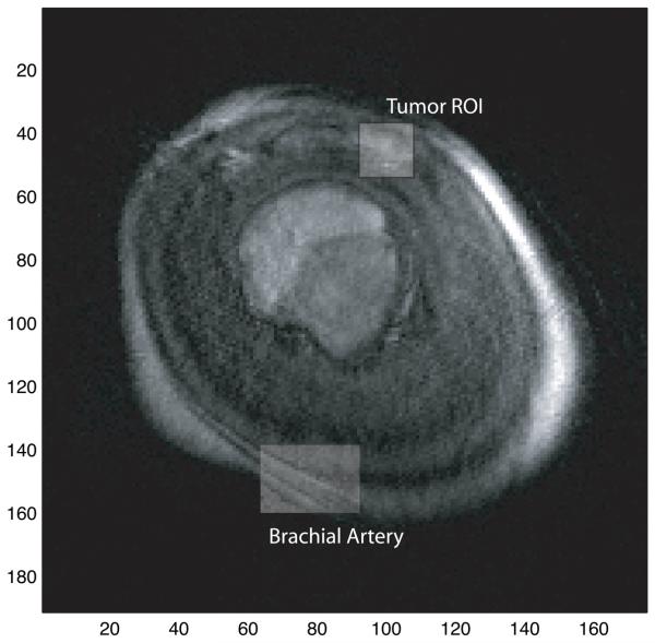
A post-contrast slice frame of this patient's DCE-MRI data is included for reference. The brachial artery, from which the measured AIF was obtained, and the tumor ROI are highlighted.

References

- 1.Tofts PS, Brix G, Buckley DL, Evelhoch JL, Henderson E, Knopp MV, Larsson HB, Lee TY, Mayr NA, Parker GJ, Port RE, Taylor J, Weisskoff RM. Estimating kinetic parameters from dynamic contrast-enhanced T(1)-weighted MRI of a diffusable tracer: standardized quantities and symbols. J Magn Reson Imaging. 1999;10(3):223–232. doi: 10.1002/(sici)1522-2586(199909)10:3<223::aid-jmri2>3.0.co;2-s. [DOI] [PubMed] [Google Scholar]
- 2.Chen JJ, Smith MR, Frayne R. The impact of partial-volume effects in dynamic susceptibility contrast magnetic resonance perfusion imaging. J Magn Reson Imaging. 2005;22(3):390–399. doi: 10.1002/jmri.20393. [DOI] [PubMed] [Google Scholar]
- 3.Wendland MF, Saeed M, Yu KK, Roberts TP, Lauerma K, Derugin N, Varadarajan J, Watson AD, Higgins CB. Inversion recovery EPI of bolus transit in rat myocardium using intravascular and extravascular gadolinium-based MR contrast media: dose effects on peak signal enhancement. Magn Reson Med. 1994;32(3):319–329. doi: 10.1002/mrm.1910320307. [DOI] [PubMed] [Google Scholar]
- 4.Parker GJ, Roberts C, Macdonald A, Buonaccorsi GA, Cheung S, Buckley DL, Jackson A, Watson Y, Davies K, Jayson GC. Experimentally-derived functional form for a population-averaged high-temporal-resolution arterial input function for dynamic contrast-enhanced MRI. Magn Reson Med. 2006;56(5):993–1000. doi: 10.1002/mrm.21066. [DOI] [PubMed] [Google Scholar]
- 5.Yang C, Karczmar GS, Medved M, Stadler WM. Estimating the arterial input function using two reference tissues in dynamic contrast-enhanced MRI studies: fundamental concepts and simulations. Magn Reson Med. 2004;52(5):1110–1117. doi: 10.1002/mrm.20243. [DOI] [PubMed] [Google Scholar]
- 6.Yang C, Karczmar GS, Medved M, Stadler WM. Multiple reference tissue method for contrast agent arterial input function estimation. Magn Reson Med. 2007;58(6):1266–1275. doi: 10.1002/mrm.21311. [DOI] [PubMed] [Google Scholar]
- 7.Yankeelov TE, Luci JJ, Lepage M, Li R, Debusk L, Lin PC, Price RR, Gore JC. Quantitative pharmacokinetic analysis of DCE-MRI data without an arterial input function: a reference region model. Magn Reson Imaging. 2005;23(4):519–529. doi: 10.1016/j.mri.2005.02.013. [DOI] [PubMed] [Google Scholar]
- 8.Zhou R, Pickup S, Yankeelov TE, Springer CS, Jr., Glickson JD. Simultaneous measurement of arterial input function and tumor pharmacokinetics in mice by dynamic contrast enhanced imaging: effects of transcytolemmal water exchange. Magn Reson Med. 2004;52(2):248–257. doi: 10.1002/mrm.20143. [DOI] [PubMed] [Google Scholar]
- 9.Riabkov DY, DiBella EV. Estimation of kinetic parameters without input functions: analysis of three methods for multichannel blind identification. IEEE Trans Biomed Eng. 2002;49(11):1318–1327. doi: 10.1109/TBME.2002.804588. [DOI] [PubMed] [Google Scholar]
- 10.Calamante F, Morup M, Hansen LK. Defining a local arterial input function for perfusion MRI using independent component analysis. Magn Reson Med. 2004;52(4):789–797. doi: 10.1002/mrm.20227. [DOI] [PubMed] [Google Scholar]
- 11.Calamente F. Bolus Dispersion Issues Related to the Quantification of Perfusion MRI Data. Journal of Magnetic Resonance Imaging. 2005;22:718–722. doi: 10.1002/jmri.20454. [DOI] [PubMed] [Google Scholar]
- 12.Wang Y, Huang W, Panicek DM, Schwartz LH, Koutcher JA. Feasibility of using limited-population-based arterial input function for pharmacokinetic modeling of osteosarcoma dynamic contrast-enhanced MRI data. Magn Reson Med. 2008;59(5):1183–1189. doi: 10.1002/mrm.21432. [DOI] [PMC free article] [PubMed] [Google Scholar]
- 13.Schabel MC, Parker DL. Uncertainty and bias in contrast concentration measurements using spoiled gradient echo pulse sequences. Phys Med Biol. 2008;53(9):2345–2373. doi: 10.1088/0031-9155/53/9/010. [DOI] [PMC free article] [PubMed] [Google Scholar]
- 14.Schabel MC, Morrell GR. Uncertainty in T(1) mapping using the variable flip angle method with two flip angles. Phys Med Biol. 2008;54(1):N1–N8. doi: 10.1088/0031-9155/54/1/N01. [DOI] [PubMed] [Google Scholar]
- 15.Carroll TJ, Rowley HA, Haughton VM. Automatic calculation of the arterial input function for cerebral perfusion imaging with MR imaging. Radiology. 2003;227(2):593–600. doi: 10.1148/radiol.2272020092. [DOI] [PubMed] [Google Scholar]
- 16.Murase K. Efficient method for calculating kinetic parameters using T1-weighted dynamic contrast-enhanced magnetic resonance imaging. Magn Reson Med. 2004;51(4):858–862. doi: 10.1002/mrm.20022. [DOI] [PubMed] [Google Scholar]
- 17.Yankeelov TE, Cron GO, Addison CL, Wallace JC, Wilkins RC, Pappas BA, Santyr GE, Gore JC. Comparison of a reference region model with direct measurement of an AIF in the analysis of DCE-MRI data. Magn Reson Med. 2007;57(2):353–361. doi: 10.1002/mrm.21131. [DOI] [PubMed] [Google Scholar]
- 18.Yankeelov TE, DeBusk LM, Billheimer DD, Luci JJ, Lin PC, Price RR, Gore JC. Repeatability of a reference region model for analysis of murine DCE-MRI data at 7T. J Magn Reson Imaging. 2006;24(5):1140–1147. doi: 10.1002/jmri.20729. [DOI] [PubMed] [Google Scholar]
- 19.Feng D, Wong KP, Wu CM, Siu WC. A technique for extracting physiological parameters and the required input function simultaneously from PET image measurements: theory and simulation study. IEEE Trans Inf Technol Biomed. 1997;1(4):243–254. doi: 10.1109/4233.681168. [DOI] [PubMed] [Google Scholar]
- 20.Wong KP, Feng D, Meikle SR, Fulham MJ. Simultaneous estimation of physiological parameters and the input function--in vivo PET data. IEEE Trans Inf Technol Biomed. 2001;5(1):67–76. doi: 10.1109/4233.908397. [DOI] [PubMed] [Google Scholar]
- 21.Cheng HL. Investigation and optimization of parameter accuracy in dynamic contrast-enhanced MRI. J Magn Reson Imaging. 2008;28(3):736–743. doi: 10.1002/jmri.21489. [DOI] [PubMed] [Google Scholar]
- 22.Schmitt M, Viallon M, Thelen M, Schreiber WG. Quantification of myocardial blood flow and blood flow reserve in the presence of arterial dispersion: a simulation study. Magn Reson Med. 2002;47(4):787–793. doi: 10.1002/mrm.10115. [DOI] [PubMed] [Google Scholar]