Multimodal functional imaging using fMRI-informed regional EEG/MEG source estimation

Abstract

We propose a novel method, fMRI-Informed Regional Estimation (FIRE), which utilizes information from fMRI in E/MEG source reconstruction. FIRE takes advantage of the spatial alignment between the neural and the vascular activities, while allowing for substantial differences in their dynamics. Furthermore, with a region-based approach, FIRE estimates the model parameters for each region independently. Hence, it can be efficiently applied on a dense grid of source locations. The optimization procedure at the core of FIRE is related to the re-weighted minimum-norm algorithms. The weights in the proposed approach are computed from both the current source estimates and fMRI data, leading to robust estimates in the presence of silent sources in either fMRI or E/MEG measurements. We employ a Monte Carlo evaluation procedure to compare the proposed method to several other joint E/MEG-fMRI algorithms. Our results show that FIRE provides the best trade-off in estimation accuracy between the spatial and the temporal accuracy. Analysis using human E/MEG-fMRI data reveals that FIRE significantly reduces the ambiguities in source localization present in the minimum-norm estimates, and that it accurately captures activation timing in adjacent functional regions.

Introduction

The principal difficulty in interpreting electroencephalography (EEG) and magnetoencephalography (MEG) data stems from the ill-posed nature of the electromagnetic inverse problem: infinitely many spatial current patterns can give rise to identical measurements (Hadamard, 1902; Hämäläinen et al., 1993). Additional assumptions about spatial current patterns, such as minimum energy (or ↕₂-norm) (Hämäläinen and Ilmoniemi, 1984; Wang et al., 1993) and minimum current (Uutela et al., 1999; Ou et al., 2009a), must be incorporated into the reconstruction process to obtain a unique estimate (Baillet et al., 2001). The corresponding estimation methods belong to the class of algorithms that model the sources as a spatial distribution, in contrast to the dipole fitting approach where the E/MEG data is explained by a small number of current dipole sources (Wood, 1982; Scherg and Von Cramon, 1985; Mosher et al., 1992). In this work, we focus on the distributed approach and aim to characterize activations with non-trivial spatial extent.

In addition to these general assumptions about the spatial patterns of activation, specific prior knowledge about activation locations can be obtained from other imaging modalities. Among them, functional Magnetic Resonance Imaging (fMRI) provides the most relevant information for the reconstruction due to its good spatial resolution. fMRI measures the hemodynamic activity, which indirectly reflects the neural activity measured by E/MEG. Extensive studies of neurovascular coupling have demonstrated similarity in spatial patterns of these two types of activations (Logothetis and Wandell, 2004; Ou et al., 2009b). However, the dynamics of the neural and the vascular activities differ substantially, and their exact relationship is yet to be characterized in full, (see, e.g., Ou et al., 2009b). In addition to the differences in their physiological origins, E/MEG and fMRI have different sensitivity characteristics. For example, a brief transient neural activity may be difficult to detect in fMRI while a sustained weak neural activity may lead to relatively strong fMRI signals, but might have a poor signal-to-noise ratio in E/MEG.

The most straightforward way to incorporate fMRI information into E/MEG inverse estimation is the fMRI-weighted minimum-norm estimation (fMNE) (Liu et al., 1998; Ahlfors and Simpson, 2004). This method uses a thresholded statistical parametric map (SPM) from fMRI analysis to construct weights for the standard minimum-norm estimation (MNE), leading to significant improvements when the SPM is accurate. However, the weights depend on arbitrary choices of the threshold and of the weighting parameters. Moreover, these weights are assumed to be identical for all time points in the E/MEG source estimation, causing excessive bias in the estimated source timecourses. Sato et al. (2004) combined the automatic relevance determination (ARD) framework and fMNE to achieve more focal estimates. In this method, which we will refer to as fARD, the parameters of a hyper-prior are set based on the thresholded SPM. Similar to fMNE, fARD depends on the arbitrary choice of the threshold for SPMs. fARD can be viewed as a “soft” variant of fMNE from the modeling perspective; its inference procedure often leads to spatially sparse solutions (Wipf and Rao, 2004). The main limitation of fARD is that the estimates may be temporally unstable, often reflected in the “spiky” estimated timecourses. fMRI information has also been incorporated into the dipole fitting approach as a constraint (George et al., 1995; Fujimaki et al., 2002; Vanni et al., 2004) or a probabilistic prior (Jun et al., 2008).

Here, we propose a novel method, the fMRI-Informed Regional Estimation (FIRE), to improve the accuracy of the E/MEG source estimates. Fig. 1 illustrates the model assumptions of FIRE. The regions indicated by different colors are chosen based on the subject-specific cortical parcellation. In this work, we choose to employ the parcellation produced by FreeSurfer (Fischl et al., 2002), but the method can be readily applied with other parcellation models. Since the relationship between the dynamics of the evoked neural and the evoked vascular signals is largely unknown, we only model the similarity of spatial patterns in the two processes, in contrast to a previously reported Kalman filtering approach in Deneux and Faugeras (2006) and Liu and He (2008). Furthermore, we expect the shape of the activation timecourses to vary across brain regions, especially for the neural activation. To account for this fact, FIRE treats the temporal dynamics in different brain regions independently. In other words, there is no constraint imposing similarity of the activation timecourses across regions. We assume the shape of the activation timecourses to be constant within a brain region, modulated by a set of location-specific latent variables. Handling the temporal dynamics of the two types of activities separately while exploiting their common spatial pattern preserves the temporal resolution of E/MEG and helps to achieve accurate source localization.

Fig. 1.

Graphical illustration of the model assumptions in FIRE. The anatomical regions of the left hemisphere are depicted in the middle of the figure. Region-specific neural waveforms (top two panels) and the vascular waveforms (bottom two panels) for two separate regions are shown in black. Location-specific current timecourses and fMRI timecourses for two locations in each of the two highlighted regions are shown in blue and green. The current timecourses and the fMRI timecourses are scaled versions of the corresponding region-specific waveforms.

The prior on the latent variables encourages spatially smooth current estimates within a brain region. The prior also encourages the number of activated regions to be small, similar to the ARD approach (Sato et al., 2004; Wipf and Nagarajan, 2009), except that our prior is applied to each brain region rather than to each location. Both the activation timecourse model and the choice of brain regions in FIRE are similar to those employed in recent work by Daunizeau et al. (2007). However, Daunizeau et al. aim to symmetrically infer brain activities visible in either EEG or fMRI data, resulting in an extra random variable to model the vascular activity. The confidence of the estimated brain activation is reduced when there are discrepancies between the EEG and the fMRI measurements. Furthermore, due to the complexity of this model, the estimation is limited to a coarse source space, effectively underutilizing the high spatial resolution provided by fMRI measurements. Instead of aiming at symmetrical inference, we focus on the estimation of current sources. We incorporate the fMRI information to reduce ambiguities in source localization typically present in E/MEG source estimation.

To fit the model to the data, we use the coordinate descent method, alternating between the estimation of current sources and that of other model parameters. This iterative update scheme is similar to the re-weighted MNE methods, such as the FOCal Underdetermined System Solver (FOCUSS) (Gorodnitsky and Rao, 1997). In contrast to the re-weighted MNE, in our method the weights are jointly determined using both the estimated neural activity and the vascular activity measured by fMRI. Moreover, the estimates at different time points influence each other. The computation of the weights is related to problems arising in continuous Gaussian mixture modeling, which can be efficiently optimized using the expectation–maximization (EM) algorithm (Dempster et al., 1977).

This paper extends the preliminary results reported in the conference paper (Ou et al., 2009c). Here we include detailed derivations of the inference procedure and a modified version of FIRE with a different initialization. We also present a more extensive experimental evaluation, including Monte Carlo simulations and experiments with human data based on somatosensory and attention-shift auditory paradigms. In the following, we first discuss the model underlying FIRE, the inference procedure, and the implementation details. We then present the experimental comparisons between FIRE and prior methods for joint E/MEG-fMRI analysis using both simulated and human data, followed by a discussion and conclusions.

Methods

In this section, we first present the model assumptions of FIRE by dissecting its graphical model shown in Fig. 2. We then discuss the priors, the parameter setting, and the inference procedure to estimate the current source distribution.

Fig. 2.

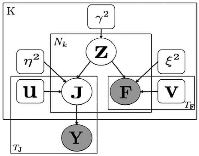
Graphical interpretation of FIRE. Circular nodes indicate random variables; square nodes indicate model parameters. The hidden activity z models the neurovascular coupling relationship. The hidden current source distribution J is measured by E/MEG, producing observation Y. F denotes fMRI measurements. Vectors u and v are the unknown region-specific neural and vascular waveforms, respectively. The inner plate represents N_k vertices in region k; the outer plate represents K regions. The bottom left and right plates represent T_J and T_F time points in the neural and the vascular measurements, respectively.

Neurovascular coupling and data models

We assume that the source space comprises N discrete locations on the cortex parceled into K brain regions. We denote the set indexing the discrete locations in region k by P_k and the cardinality of P_k by N_k. Hence, the outer plate in Fig. 2 describes K regions, and the inner plate captures N_k locations in region k.

The shapes of the source timecourses are identical within a region but may vary across regions. Specifically, we let u_k and v_k be the unknown waveforms in region k, associated with the neural and vascular activities, respectively. Examples u_k and v_k in two separate brain regions are illustrated as the black timecourses in Fig. 1. We model the strengths of neural and the vascular activities through a hidden vector variable Z = [z₁, z₂,…, z_N]^T, where z_n indicates the activation strength at location n on the cortical surface. Thus, the probabilistic model for the neural activation timecourse j_n and the vascular activation timecourse f_n at location n in region k can be expressed as

$$p\left({\mathbf{j}}_n,{\mathbf{f}}_n\mid z_n;{\mathbf{u}}_k,{\mathbf{v}}_k,{\eta }_k^2,{\xi }_k^2\right)=p\left({\mathbf{j}}_n\mid z_n;{\mathbf{u}}_k,{\eta }_k^2\right)p\left({\mathbf{f}}_n\mid z_n;{\mathbf{v}}_k,{\xi }_k^2\right)$$ (1)

$$=\mathcal{N}\left({\mathbf{j}}_n;z_n{\mathbf{u}}_k,{\eta }_k^2\mathbf{I}\right)\mathcal{N}\left({\mathbf{f}}_n;z_n{\mathbf{v}}_k,{\xi }_k^2\mathbf{I}\right),$$ (2)

where ${\eta }_k^2$ and ${\xi }_k^2$ are noise variances. The blue and green timecourses in Fig. 1 represent examples of j_n and f_n for two locations within each region. Note that our neurovascular coupling model captures only the spatial alignment between the two types of activities; it does not impose temporal similarity of the signals. The neural timecourses j_n and the vascular signals f_n are conditionally independent given the hidden variable for brain activity z_n. Although the parcellation is optimal when each parcel includes one type of neural and vascular waveform, our experimental results show that FIRE’s performance is comparable to other methods when multiple waveforms are present within a parcel.

In the model description below, we construct all matrices such that rows represent locations or sensors and columns represent time points. Thus, we let N × T_J matrix J = [j₁, j₂, …, j_N]^T be the hidden neural current on the cortex for all T_J time points. We assume that the vascular signal f_n at location n is directly observable via fMRI. We let N × T_F matrix F = [f₁, f₂, …, f_N]^T be the fMRI measurements on the cortex at all T_F time points.

The neural currents j_n detected with E/MEG are characterized by the standard observation model. We let M × T_J matrix Y = [y(1), y(2), …, y(T_J)] be the E/MEG measurements at all T_J time points. Column t of matrix J, j(t), denotes the neural current distribution at time t. The quasi-static approximation of Maxwell’s equations states that E/MEG signals at time t are instantaneous linear combinations of the currents at different locations in the source space:

$$\mathbf{y}(t)=\mathbf{Aj}(t)+\mathbf{e}(t)\forall t=1,2,\dots ,T_{\mathbf{J}},$$ (3)

where e(t) is the measurement noise at time t. The M × N forward matrix A captures the electromagnetic properties of the head, the geometry of the sensors, and the locations of the sources. Similar to other source estimation methods, the forward matrix A is assumed to be known. We assume spatial whitening in the measurement (sensor) space so that e(t) ~ (0, I). The number of sources N (~10⁴) is much larger than the number of measurements M (~10²), leading to an infinite number of solutions satisfying Eq. (3) even for e(t) = 0. The plate at the bottom left corner of Fig. 2 corresponds to T_J temporal samples. In general, j_n should be modeled as three timecourses corresponding to the three Cartesian components of the current. However, due to the columnar organization of the cortex, we can further constrain the current orientation to be perpendicular to the cortical surface and consider a scalar current value at each location.

Priors and parameter settings

To encourage the activation patterns to vary smoothly in space within a region, we impose a prior on the modulating variables Z. Specifically, we define z = {z_n}_{n ⊂ Pk} and assume

$$p\left(\mathbf{Z};{\{{\gamma }_k\}}_{k=1}^K\right)=\prod _{k=1}^{K}p\left({\underset{\_}{\mathbf{z}}}_k;{\mathbf{\gamma }}_k\right)=\prod _{k=1}^K\mathcal{N}\left(0,{\gamma }_k^2{\mathbf{\Gamma }}_k\right),$$ (4)

where the variance ${\gamma }_k^2$ indirectly models the strength of the activation magnitude z_n in region k, and Γ_k is a fixed matrix that acts as a regularizer by penalizing the sum of squared differences between neighboring locations. This spatial prior is particularly important for the brain regions where vascular activity is too weak to measure, but the neural activity can be detected by E/MEG. Without this prior, the estimated current source may have an unrealistic spatial distribution due to the ill-posed nature of the E/MEG inverse problem.

Our Γ_k is similar to the regularizer used in the Low Resolution Brain Electromagnetic Tomography (LORETA) (Pascual-Marqui et al., 1994), except that we apply Γ_k to individual brain regions while LORETA’s spatial regularizer is applied to the whole brain. We assume separate variance ${\gamma }_k^2$ for different brain regions since the strength of the currents is expected to vary significantly between regions with and without active sources. This choice is similar to the recent work in the application of ARD to E/MEG reconstruction (Sato et al., 2004; Wipf and Nagarajan, 2009), except that their work assumes independent variance γ² for each location in the brain.

Since the forward matrix A is underdetermined, the current distribution J produced by our neurovascular coupling model can fully explain the E/MEG data. In other words, without the noise term ${\eta }_k^2$ (i.e., j_n = z_nu_k), the fMRI data can exert too much influence on the reconstruction results. Although we can estimate the noise variance of the current source time courses ${\eta }_k^2$ by extending the inference procedure, we find the corresponding estimate unstable without a prior. Based on the preliminary empirical testing, we fix ${\eta }_k^2=1$. With proper temporal whitening of the fMRI data, we can also assume that ${\xi }_k^2={\eta }_k^2$. Fixing ${\eta }_k^2={\xi }_k^2$ helps to significantly reduce the computational burden of the estimation.

To summarize, our model can be mathematically expressed as

$$p(\mathbf{F},\mathbf{Y},\mathbf{J},\mathbf{Z};\mathbf{\Theta })=p(\mathbf{Y}\mid \mathbf{J})p(\mathbf{J},\mathbf{F}\mid \mathbf{Z};\mathbf{\Theta })p(\mathbf{Z};\mathbf{\Theta }),$$ (5)

where Θ = [θ₁, θ₂, …, θ_K] is the combined set of parameters, and ${\theta }_k=[{\mathbf{u}}_k,{\mathbf{v}}_k,{\gamma }_k^2]$ is the set of parameters for region k. p(Y|J) is the E/MEG data model in Eq. (3). As shown in Fig. 2, the E/MEG observation Y is conditionally independent of other variables given the hidden source currents J. p(J, F|Z; Θ) is our neurovascular coupling model in Eq. (1), and p(Z; Θ) is the prior on Z in Eq. (4). Combining these elements of the joint likelihood model, we obtain

$$\begin{array}{l}logp(\mathbf{Y},\mathbf{J},\mathbf{F},\mathbf{Z};\mathbf{\Theta })=logp(\mathbf{Y}\mid \mathbf{J})+logp(\mathbf{J},\mathbf{F}\mid \mathbf{Z};\mathbf{\Theta })+logp(\mathbf{Z};\mathbf{\Theta })\\ =\sum _{t=1}^{T_{\mathbf{J}}}log\mathcal{N}(\mathbf{y}(t);\mathbf{Aj}(t),\mathbf{I})+\sum _{k=1}^K\sum _{n=1}^{N_k}[log\mathcal{N}({\mathbf{j}}_n;z_n{\mathbf{u}}_k,\mathbf{I})+log\mathcal{N}({\mathbf{f}}_n;z_n{\mathbf{v}}_k,\mathbf{I})]+\sum _{k=1}^{K}log\mathcal{N}\left({\underset{\_}{\mathbf{z}}}_k;\mathbf{0};{\gamma }_k^2{\mathbf{\Gamma }}_k\right)\\ =-\frac{1}{2}\left[M{T}_{\mathbf{J}}log(2\pi )+\sum _{t=1}^{T_{\mathbf{J}}}{\left|\right|\mathbf{y}(t)-\mathbf{Aj}(t)\left|\right|}^2\right]-\frac{1}{2}\sum _{k=1}^K\left[N_k{T}_{\mathbf{J}}log(2\pi )+\sum _{n\in P_k}{\left|\right|{\mathbf{f}}_n-z_n{\mathbf{v}}_k\left|\right|}^2+N_k{T}_{\mathbf{F}}log(2\pi )+\sum _{n\in P_k}{\left|\right|{\mathbf{j}}_n-z_n{\mathbf{u}}_k\left|\right|}^2\right]-\frac{1}{2}\sum _{k=1}^K\left[N_{k}log(2\pi )+N_{k}log\left({\gamma }_k^2\right)+log(det({\mathbf{\Gamma }}_k))+\frac{{\underset{\_}{\mathbf{z}}}_k^T{\mathbf{\Gamma }}_k^{-1}{\underset{\_}{\mathbf{z}}}_k}{{\gamma }_k^2}\right]\end{array}$$ (6)

where det (·) denotes matrix determinant. Note that although the latent activation strength Z is independent across regions a priori, the posterior estimates for J, Z, and Θ are spatially dependent due to the measurements Y.

Inference

Our goal is to estimate the current source J and the timecourses u and v. A standard inference procedure is to compute the maximum likelihood (ML) estimate of Θ while jointly considering the current source distribution J and the activation strength Z as hidden variables, followed by a maximum a posteriori (MAP) estimation of J. However, this leads to a computationally intractable algorithm, as we discuss in Discussion. Instead, we alternate the optimization between estimating J and estimating Θ. While estimating Θ, we treat the activation strength Z as an auxiliary variable, and marginalize it out in the analysis. Our inference procedure can be thus formulated as

$$\{{\mathbf{J}}^{\ast },{\mathbf{\Theta }}^{\ast }\}=\underset{\mathbf{J},\mathbf{\Theta }}{argmax}logp(\mathbf{F},\mathbf{Y},\mathbf{J};\mathbf{\Theta })$$ (7)

$$=\underset{\mathbf{J},\mathbf{\Theta }}{argmax}log{\int }_{\mathbf{Z}}p(\mathbf{Y}\mid \mathbf{J})p(\mathbf{F},\mathbf{J}\mid \mathbf{Z};\mathbf{\Theta })p(\mathbf{Z};\mathbf{\Theta })d\mathbf{Z}$$ (8)

$$=\underset{\mathbf{J},\mathbf{\Theta }}{argmax}logp(\mathbf{Y}\mid \mathbf{J})+logp(\mathbf{F},\mathbf{J};\mathbf{\Theta }).$$ (9)

In Eq. (9), p(F, J; Θ) acts as the prior for J. Since both J and F are linear functions of Z, p(F, J; Θ) is a continuous Gaussian mixture model.

The difficulty in estimating the proposed model from the data is caused by the interactions between space and time variables, as reflected by the intersection of the temporal plates and the spatial plates in Fig. 2. It is easy to see from Eq. (3) that the output of a given E/MEG sensor is a mixture of signals from the entire source space. Moreover, F, J, and Y are jointly Gaussian. The correlation between different time points (i.e., between two E/MEG time points, between two fMRI time points, and between E/MEG and fMRI time points) is generally not zero. Hence, the inference must be performed for all time points and all locations simultaneously. FIRE is thus substantially more computationally demanding than the standard temporally independent E/MEG estimation or voxel-wise fMRI analysis that ignore these dependencies in modeling the observed signals. The benefit of this increased computational burden is more accurate inference across time points.

Due to the special structure of our model, we can derive an efficient gradient descent method with two alternating steps. In the first step, we fix Θ and derive a closed-form solution for J. In the second step, we fix J and show that Θ can be efficiently estimated via the EM algorithm (Dempster et al., 1977).

For a fixed Θ = Θ̂, p(F, Y, J; Θ̂) is a jointly Gaussian distribution. As shown in Appendix A, the estimate of J is therefore equal to its conditional mean:

$$\text{vec}\left(\widehat{\mathbf{J}}\right)=arg\underset{\mathbf{J}}{max}logp\left(\mathbf{F},\mathbf{Y},\mathbf{J};\widehat{\mathbf{\Theta }}\right)=E\left[\mathbf{J}\mid \mathbf{F},\mathbf{Y};\widehat{\mathbf{\Theta }}\right]={\mathbf{\Gamma }}_{\mathbf{W},\mathbf{J}}^T{\mathbf{\Gamma }}_{\mathbf{W}}^{-1}\mathbf{W},$$ (10)

where W^T = [(vec(F))^T(vec(Y))^T] includes both E/MEG and fMRI measurements. Operator vec(·) concatenates the columns of a matrix into a vector. Γ_W is the covariance matrix of W, and Γ_W,J is the cross-covariance matrix between W and vec(J). Appendix A presents the detailed derivations for Γ_W and Γ_W,J. Eq. (10) implies that E/MEG and fMRI measurements jointly determine the estimate of the neural activity. This equation is similar to the standard MNE solution (Hämäläinen et al., 1993), but also includes the correlation between the observations Y and F and the correlation among different time points of the neural current J.

For a fixed J = Ĵ, we estimate the parameters Θ:

$$\widehat{\mathrm{\Theta }}=arg\underset{\mathbf{\Theta }}{max}logp\left(\mathbf{F},\widehat{\mathbf{J}};\mathbf{\Theta }\right)=arg\underset{\mathbf{\Theta }}{max}\sum _{k=1}^{K}logp\left({\left\{{\mathbf{f}}_n,{\widehat{\mathbf{j}}}_n\right\}}_{n\in P_k};{\theta }_k\right).$$ (11)

It is easy to see that this optimization can be done for each region separately:

$${\widehat{\theta }}_k=arg\underset{{\theta }_k}{max}logp\left({\left\{{\mathbf{f}}_n,{\widehat{\mathbf{j}}}_n\right\}}_{n\in P_k};{\theta }_k\right)\forall k=1,\dots ,K.$$ (12)

As can be seen in Fig. 2, when the current distribution J is fixed, the E/MEG measurement Y does not provide additional information for the parameter estimation. Furthermore, each set of parameters θ_k can be efficiently estimated using the EM algorithm (Dempster et al., 1977) by re-introducing the latent variable z_k that describes activation strength of vertices within region k. This method can be thought of as an extension of the EM algorithm for probabilistic PCA (Tipping and Bishop, 1999) to two sets of data (Bach and Jordan, 2005).

Specifically, the parameter estimates θ̂_k for region k can be obtained by optimizing the lower bound of the log-probability:

$$logp\left({\left\{{\mathbf{f}}_n,{\widehat{\mathbf{j}}}_n\right\}}_{n\in P_k};{\theta }_k\right)\ge {\int }_{{\underset{\_}{\mathbf{z}}}_k}q\left({\underset{\_}{\mathbf{z}}}_k\right)logp\left({\left\{{\mathbf{f}}_n,{\widehat{\mathbf{j}}}_n\right\}}_{n\in P_k},{\underset{\_}{\mathbf{z}}}_k;{\theta }_k\right)d{\underset{\_}{\mathbf{z}}}_k-{\int }_{{\underset{\_}{\mathbf{z}}}_k}q\left({\underset{\_}{\mathbf{z}}}_k\right)logp\left(q\left({\underset{\_}{\mathbf{z}}}_k\right)\right)d{\underset{\_}{\mathbf{z}}}_k,$$ (13)

where q(z_k) = p(z_k|{f_n, j_n}_{n ∈ Pk}; θ̃_k) is the posterior probability computed in the E-step, and θ̃_k is the estimate from the last EM iteration. Since {f_n, ĵ_n}_{n ∈ Pk} and zk are jointly Gaussian, q(zk) is also a Gaussian distribution, and the M-step update depends only on the first- and the second-order statistics of z_k. Due to this special structure, we first derive the M-step, followed by the E-step. To simplify notation, we use <·>_q to denote the expectation with respect to the posterior distribution q(z_k), i.e., ${\langle ·\rangle }_q\triangleq E[·\mid {\{{\mathbf{f}}_n,{\mathbf{j}}_n\}}_{n\in P_k};{\stackrel{\sim }{\theta }}_k]$.

In the M-step, we fix q(z_k) and optimize the right-hand side of Eq. (13), and get

$${\widehat{\theta }}_k=arg\underset{{\theta }_k}{max}{\int }_{{\underset{\_}{\mathbf{z}}}_k}q\left({\underset{\_}{\mathbf{z}}}_k\right)logp\left({\left\{{\mathbf{f}}_n,{\widehat{\mathbf{j}}}_n\right\}}_{n\in P_k},z_n;{\theta }_k\right)d{\underset{\_}{\mathbf{z}}}_k$$ (14)

$$=arg\underset{{\theta }_k}{max}{N}_k\left({\mathbf{v}}_k^T{\mathbf{f}}_n+{\mathbf{u}}_k^T{\widehat{\mathbf{j}}}_n\right){\langle z_n\rangle }_q-\frac{N_k}{2}\left({\mathbf{v}}_k^T{\mathbf{v}}_k+{\mathbf{u}}_k^T{\mathbf{u}}_k\right){\langle z_n^2\rangle }_q-\frac{1}{2}\frac{{\langle {\underset{\_}{\mathbf{z}}}_k^T{\mathbf{\Gamma }}_k^{-1}{\underset{\_}{\mathbf{z}}}_k\rangle }_q}{{\gamma }_k^2}-N_{k}log{\gamma }_k^2.$$ (15)

The detailed derivations of Eq. (15) are shown in Appendix B. Setting the derivatives of Eq. (15) with respect to the model parameter vector ${\theta }_k=[{\mathbf{u}}_k,{\mathbf{v}}_k,{\gamma }_k^2]$ to zero, we arrive at the update rules:

$${\widehat{\mathbf{u}}}_k\leftarrow \frac{{\sum }_{n\in P_k}{\langle z_n\rangle }_q{\widehat{\mathbf{j}}}_n}{tr\left({\langle {\underset{\_}{\mathbf{z}}}_k{\underset{\_}{\mathbf{z}}}_k^T\rangle }_q\right)},{\widehat{\mathbf{v}}}_k\leftarrow \frac{{\sum }_{n\in P_k}{\langle z_n\rangle }_q{\mathbf{f}}_n}{tr\left({\langle {\underset{\_}{\mathbf{z}}}_k{\underset{\_}{\mathbf{z}}}_k^T\rangle }_q\right)},{\widehat{\gamma }}_k^2\leftarrow \frac{{\langle {\underset{\_}{\mathbf{z}}}_k^T{\mathbf{\Gamma }}_k^{-1}{\underset{\_}{\mathbf{z}}}_k\rangle }_q}{N_k}.$$ (16)

Since the M-step depends only on quantities ${\langle {\underset{\_}{\mathbf{z}}}_k{\underset{\_}{\mathbf{z}}}_k^{\text{T}}\rangle }_q$, <z_k>_q, and ${\langle {\underset{\_}{\mathbf{z}}}_k^{\text{T}}{\mathbf{\Gamma }}_k^{-1}{\underset{\_}{\mathbf{z}}}_k\rangle }_q$, we only need to evaluate those quantities in the E-step:

$${\langle {\underset{\_}{\mathbf{z}}}_k{\underset{\_}{\mathbf{z}}}_k^T\rangle }_q\leftarrow {\left[\frac{1}{{\gamma }_k^2}{\mathbf{\Gamma }}_k^{-1}+\left({\mathbf{v}}_k^T{\mathbf{v}}_k+{\mathbf{u}}_k^T{\mathbf{u}}_k\right)\mathbf{I}\right]}^{-1}$$ (17)

$${\langle {\underset{\_}{\mathbf{z}}}_k\rangle }_q\leftarrow {\langle {\underset{\_}{\mathbf{z}}}_k{\underset{\_}{\mathbf{z}}}_k^T\rangle }_q{\left[\left({\mathbf{v}}_k^T{\mathbf{f}}_1+{\mathbf{u}}_k^T{\widehat{\mathbf{j}}}_1\right),\dots ,\left({\mathbf{v}}_k^T{\mathbf{f}}_{N_k}+{\mathbf{u}}_k^T{\widehat{\mathbf{j}}}_{N_k}\right)\right]}^T$$ (18)

$${\langle {\underset{\_}{\mathbf{z}}}_k^T{\mathbf{\Gamma }}_k^{-1}{\underset{\_}{\mathbf{z}}}_k\rangle }_q\leftarrow {\langle {\underset{\_}{\mathbf{z}}}_k\rangle }_q^T{\mathbf{\Gamma }}_k^{-1}{\langle {\underset{\_}{\mathbf{z}}}_k\rangle }_q+\text{tr}\left({\mathbf{\Gamma }}_k^{-1}{\langle {\underset{\_}{\mathbf{z}}}_k{\underset{\_}{\mathbf{z}}}_k^T\rangle }_q\right).$$ (19)

We iterate the EM algorithm until convergence which usually takes less than ten iterations. We then re-estimate J according to Eq. (10).

To summarize, the FIRE inference algorithm proceeds as follows:

1. Initialize Ĵ as the MNE estimate: J^(MNE) = A^T(AA^T + λ²I)⁻¹Y, where λ² is the regularization parameter related to the SNR of the data.

2. Repeat until convergence:

   1. Compute Θ̂ using the EM algorithm:

      1. E-step: construct ${\{q({\underset{\_}{\mathbf{z}}}_k)\}}_{k=1}^K$ (Eqs. (17)–(19))

      2. M-step: estimate parameters Θ (Eq. (16))

   2. Update Ĵ for Θ = Θ̂ (Eq. (10)).

We also examine FIRE with different initializations. In particular, we use the fMNE estimate to initialize the algorithm and refer to this method as fFIRE. The fMNE estimate can be expressed as J^(fMNE) = RA^T (ARA^T+λ²I)⁻¹Y, where R is a diagonal matrix of size N whose values depend on the thresholded fMRI-SPMs of the corresponding locations. A standard choice, as proposed in Liu et al. (1998), is 1 for locations with fMRI activation above a preselected threshold and 0.1 for those below the threshold.

Implementation

For the computation of the forward matrix A, we need to specify the E/MEG forward model and the source space. We employ the single-compartment and the three-compartment boundary-element models for MEG and EEG forward computations, respectively (Hämäläinen and Sarvas, 1989; Oostendorp and Van Oosterom, 1989). For combined E/MEG inference we employ the three-compartment model for both modalities. The source space is confined to a mesh on the cortical surface with an approximately 5-mm spacing between adjacent source space points. The cortical regions for modeling purposes are defined by parceling the cortical surface using the FreeSurfer software, resulting in 35 parcels per hemisphere (Fischl et al., 2002). The boundaries of adjacent parcels are defined along sulci. We merge adjacent parcels that contain fewer than 30 vertices.

Under the orientation constrain, most forward models A follow a local orientation convention: the currents flowing outward of the cortex are considered positive and the currents flowing inward are viewed as negative. That means if a region includes two sides of a gyrus, the positive on the two sulcal walls corresponds to currents flowing in opposite directions. Hence, the local time courses will have opposite signals violating the assumption of a single time course. In this work, we set the regional orientation reference to be the largest left singular vector of the matrix formed by the outward cortical normals within a region. We then modify the sign of the columns in the forward matrix A corresponding to vertices based on the angle between their normal vectors and the reference vector. We reverse the sign of a column if the angle between the normal and the reference vector is greater than 90°. To display the estimated current J*, we reverse the sign alternation and display results using the local orientation convention mentioned above.

We apply the standard preprocessing to fMRI data, then estimate the hemodynamic response function (HRF) at each voxel with a finite impulse response regressor covering a 20-s time window using the FS-FAST software (MGH, Boston, MA). The estimated HRF is used as the hemodynamic data f_n in our model.

For a source space of N ~ 10,000 vertices and timecourses of T_J ~ 100 and T_F ~ 10 samples, FIRE takes less than 20 iterations until the energy function is reduced by less than 0.1% in the next iteration. In each iteration of the coordinate descent algorithm, the estimation of Θ takes 30 s; the estimation of J takes 4 min on a standard PC (2.8 GHz CPU and 8 GB RAM), leading to the total run time of approximately 1.5 h. Estimating J involves an inversion of an (MT_J + NT_F) × (MT_J + NT_F) dense symmetric matrix Γ_W, which is too large to store in memory. Instead, we employ the conjugate gradient descent method to solve the corresponding system of linear equations. It usually takes 100 iterations until convergence. Using the same computational resources, the run time for fARD is shorter since it estimates the current source distribution at each time point separately, ignoring the dependencies in the signal across time. The total run time for fARD with 10 iterations is about 5 min.

Results

We first compare FIRE and fFIRE to MNE, fMNE, and fARD using simulated data, including three scenarios closely related to those typically observed in human experiments. We employ a Monte Carlo procedure to estimate performance statistics for each method. We then proceed to a comparison of the methods using human E/MEG-fMRI data from a somatosensory study and an attention-shift auditory study.

Simulation studies

To simulate MEG measurements, we created two patches on the cortical surface, with current source orientation along the outward normal to the cortical surface. As shown in the lateral–occipital view of the right hemisphere (Fig. 3), patch A contains 20 vertices and is located in the inferior parietal region. Patch B contains 32 vertices and is located in the superior parietal region. The selection of the source patches is independent of the anatomical parcellation used in the source estimation. The anatomical parcels are used in the inference only. We simulated neural and vascular timecourses in these two patches for three different scenarios: no silent activity, silent vascular activity, and silent neural activity. In the two cases with silent activities, we kept the activity of patch B unchanged while silencing neural or vascular activity in patch A. The simulated neural signals are shown as solid black lines in the rightmost column of Fig. 3. The activation maps corresponding to the peaks of the two simulated neural signals are shown in the first column.

Fig. 3.

Current source estimates in three scenarios. Lateral–occipital view of the right hemisphere is shown. Patch A and patch B are highlighted in the top left panel; the rest of the figures follow the same convention. (Top) Neither neural nor vascular activity is silent. (Middle) Vascular activity in patch A is silent. (Bottom) Neural activity in patch A is silent. The first column illustrates the simulated current distributions with a selected threshold at the peak activations. The next four columns show the estimates from MNE, fMNE, fARD, and FIRE, respectively, for the time of peak activation for each patch. Hot/cold colors correspond to outward/inward current flow. The rightmost column shows the simulated (black solid) and the estimated (dashed) timecourses from the most active vertices in patches A and B. The color of the time course matches with those used for the name of the corresponding method.

For the forward calculations, we employed the sensor configuration of the 306-channel Neuromag VectorView MEG system used in our human studies and added Gaussian noise to the signals. The resulting signals have a SNR of 3 dB, within the typical SNR range of real MEG data. Since the two patches are close to each other in the highly folded cortex and they exhibit neural activity during overlapping time intervals, it is particularly difficult to obtain accurate current source estimates for this configuration.

Columns two to five in Fig. 3 depict the current source estimates J^* obtained via different methods for the two time points corresponding to the peaks of activity. Following Liu et al. (1998), the fMNE weighting parameters are set to 1 and 0.1 for active and inactive fMRI locations, respectively. The hyper-parameters for fARD are selected according to Sato et al. (2004).¹ The results from FIRE and fFIRE are quite similar in this simulation setting. We therefore defer the evaluation of fFIRE to the Monte Carlo procedure presented later in this session. Since the estimates from different methods are not directly comparable in amplitude, the threshold for each method is chosen to be 1/6 of the maximum absolute value of the corresponding current source estimates. The rightmost column in Fig. 3 presents the estimated timecourses (dashed) of the most active vertex, in terms of energy, in both patches.

No silent activity

As shown in Fig. 3(top), the MNE estimates extend across adjacent gyri. fMNE, fARD, and FIRE correctly localize the two patches at the peak activation, but FIRE provides a better estimate of the spatial extent of the activations. The fARD estimate is unstable, as reflected by the large fluctuations in the estimated timecourses, especially in patch B (Fig. 3(top), rightmost column, green).

Silent vascular activity

When the vascular activity in patch A is silent, fMNE shows excessive bias towards patch B. Without a large weight, the amplitude of the estimated timecourses (Fig. 3(middle), rightmost column, blue) in patch A is significantly lower than the corresponding estimates in patch B. It would be therefore easy to miss neural activation in patch A when interpreting the results (column three in Fig. 3(middle)). In contrast, by combining neural and vascular information in the re-weighted scheme, FIRE avoids such a bias. Its estimate in patch A (column five) is similar to that obtained via MNE (column one). Since the weight for patch B increases and the weight for patch A decreases during the fARD updates, the estimate in patch B explains the activation in patch A. As shown in the timecourse panel, the estimated timecourse in patch B (green) is similar in shape to the simulated timecourse in patch A (black solid). The change of sign is due to the fact that the outward normals for patch A and patch B are in approximately opposite directions.

Silent neural activity

As shown in Fig. 3(bottom), all methods correctly localize the neural activity in patch B, except for the small false positive in patch A for fARD. By assigning identical weights to patches A and B, fMNE estimates a timecourse for patch A (blue) that is noisier than the corresponding one produced by FIRE (red). FIRE suppresses the weights for patch A since the current estimates in that patch are close to zero; its results are closer to the simulations.

Monte Carlo simulation

We repeated the above experiments 100 times for each of the three scenarios. For each run, the locations of the simulated patches were randomly selected on the right hemisphere. Due to their spatial extent, the selected patches are likely to span portions of multiple anatomical parcels obtained from FreeSurfer: a patch on average spans 3.5 anatomical parcels. Furthermore, in 30% of the trials in the simulation, the two selected patches cover the same anatomical parcel.

When comparing different estimation methods, we evaluated both the temporal and the spatial properties of the results. We used the correlation coefficient between the estimated timecourses and the ground truth ones, in the two patches separately, to evaluate the ability of the methods to reproduce the timecourses of the activity (Fig. 4, leftmost column). To compare spatial accuracy of the methods, we computed the receiver operating characteristic (ROC) curve (Fig. 4, middle column) and the average distance between the simulated patches and the falsely detected locations (Fig. 4, right column). To compute the ROC curve, we selected the current estimates J^* at two time points corresponding to the peak activation. For each time point, we then separately varied the threshold and compared it with the ground truth to compute the true positive and false positive rates. To compute the distance to false positives, we varied the false positive rate, and computed the average distance between the falsely detected vertices and the ground truth activation patches.

Fig. 4.

Performance statistics in the three scenarios. Left: the correlation coefficients between the estimated timecourses and the ground truth ones in patch A (top) and patch B (bottom). Middle: the ROC curves evaluated at the peak activation of the two patches. Right: the average distance from the simulated patches to the falsely detected locations.

We first focus on the temporal correlation (Fig. 4, left column). For the three scenarios, FIRE and fFIRE achieve the highest temporal correlation (approximately 0.65), for patches exhibiting both neural and vascular activities (rows 1–3 and 5). The combination of static fMRI-SPM and the shrinkage prior in the ARD framework causes unstable timecourse estimates, reflected in low temporal correlation for fARD. When the patch exhibits neural activity, but no vascular activity, the temporal correlations are similar across all source estimation algorithms we examined (approximately 0.55).

The ROC curves (Fig. 4, middle column) demonstrate that fARD, fMNE, and fFIRE achieve similar detection accuracy for patches exhibiting both neural and vascular activities. When a patch shows neural activity, but no vascular activity, all algorithms have similar detection accuracy. As shown in the right column of Fig. 4, the falsely detected locations obtained from MNE, FIRE, and fFIRE tend to be close to the ground truth patches. In contrast, the falsely detected locations for fARD are relatively far away from the simulated patches, 5 to 6 cm on average. The standard error decreases as the false positive rate increases as there are more false positives involved in the computation of the average distance. Among all algorithms that we examined, fFIRE provides the best trade-off between the spatial and the temporal accuracy.

We analyzed separately the performance of the 30% of the trials where the two source patches are located within the same anatomical parcel. Since the two activations are close to each other in space, the current estimation is particularly challenging in this case. We see significant reduction in performance across all methods, and their performance becomes more similar: the temporal correlation coefficients are 0.16 for MNE and fMNE, and 0.18 for FIRE and fFIRE; at false positive rate 0.005, the true positive rates are 0.20 for fMNE and fFIRE, 0.13 for FIRE, and 0.06 for MNE. We observe that the results for FIRE and fFIRE are quite robust with respect to the choice of anatomical parcellations. Although FIRE and fFIRE use a less-than-optimal parcellation in these 30% trials, the performance is equivalent to that of MNE and fMNE.

Human experiments

We also tested the method using human experimental data. E/MEG and fMRI measurements were obtained in separate sessions. The MEG data were acquired using a 306-channel Neuromag VectorView MEG system; the EEG data were acquired simultaneously with a 70-channel MEG-compatible EEG system. A 200 ms baseline before the stimulus was used to estimate the noise covariance matrix of the MEG sensors and EEG electrodes. fMRI data were obtained with a 3 T Siemens TimTrio scanner. Anatomical images, from a 3 T scanner, were used to construct the source space and the forward model. Informed consent in accordance with the Massachusetts General Hospital ethical committee was obtained from subjects prior to participation.

Median-nerve experiments

The median nerve at the right wrist was stimulated according to an event-related protocol, with a random inter-stimulus-interval ranging from 3 to 14 s. This stimulus activates a complex cortical network (Hari and Forss, 1999), including the contralateral primary somatosensory cortex (cSI) and bilateral secondary somatosensory cortices (cSII and iSII).

An average MEG signal, computed from approximately 100 trials, was used as the input to each method. In this experiment, EEG data were not acquired. The fMRI images were acquired using a Siemens 3 T scanner (TR = 1.5 s, 64 × 64 × 24, 3 × 3 × 6 mm³, single channel head coil).

In the leftmost column in Fig. 5, the approximate locations for cSI (solid), cSII (dashed), and iSII (dashed) are highlighted on the fMRI activation maps (p ≤ 0.005 uncorrected). Given the expected activations, we partitioned the contralateral activation into two regions, separately covering cSI and cSII. Note that in the noisy SPM, the sites of fMRI activations do not exactly agree with the locations of the expected current sources.

Fig. 5.

Human median-nerve experiments. In the first column, approximate locations for cSI (solid), cSII (dashed), and iSII (dashed) are highlighted on the fMRI activation maps (p ≤ 0.005). Columns two to five show the current estimates obtained via MNE, fMNE, fARD, FIRE, and fFIRE respectively, at 75 ms after the stimulus onset. Hot/cold colors indicate outward/inward current flow.

Columns two to five in Fig. 5 present the estimates at 75 ms after stimulus onset. At this time, cSI, cSII, and iSII should be activated. The threshold was set separately for each hemisphere since the activation in iSII is much weaker than that in cSI and cSII. For each method, the threshold is set to be 1/6 of the maximum absolute value of the corresponding current estimates. MNE produces a diffuse estimate, including physiologically unlikely activations at the gyrus anterior to the cSI area. In contrast, FIRE and fFIRE pinpoint cSI to the post-central gyrus. With the prior knowledge from fMRI, the detected cSII and iSII activations using fMNE, fARD, FIRE, and fFIRE are within the expected areas. The fMNE and fARD show stronger weighting toward the fMRI, reflected by the activations in the temporal lobes. fFIRE further detects activation in the visual area, the middle temporal area (MT) of the left hemisphere. This false detection is primarily caused by the strong activation in this area present in the initialization for fFIRE. Due to the highly folded nature of the cortex and uncertainties in MRI-fMRI registration, fMRI cannot distinguish between the walls of the central sulcus and the post-central sulcus, causing both walls to show strong vascular activity after mapping of the fMRI volume onto the cortex. Hence, fMNE, fARD, FIRE, and fFIRE estimates extend to both sulcal walls.

Attention-shift auditory experiments

An auditory attention task was utilized to investigate activations elicited by occasional attention shifting cues during dichotic stimulation. These activations were presumed to spread from the primary auditory cortex (Heschl’s gyrus, HG) to surrounding association areas within the superior temporal plane (superior temporal gyrus, STG; planum temporale, PT) (Ahveninen et al., 2006; Hart et al., 2002; Rauschecker, 1998) and the superior temporal sulcus (STS) (Altmann et al., 2008; Lu et al., 1992; Williamson et al., 1991) before extending to higher-order parietofrontal areas associated with attention shifting. Functional characterization of different subregions of the auditory cortex has been difficult in humans. In this experiment, we focus on the performance of each source estimation method in characterizing different activation patterns in the auditory cortex.

Three subjects were recruited for this study, and their task was to press a button upon hearing a target stimulus (quarter-tone or semitone deviants among standard tones) in the designated ear and to ignore sounds in the opposite ear. The stimulus of interest was an occasional “novel” buzzer sound that instructed the subject to shift attention to the cued ear. During E/MEG acquisition, the cue was presented after every 30 s. During fMRI acquisition, attention shifting cues were presented between clustered EPI acquisitions, after every other TR.

An average MEG signal, computed from approximately 40 trials, was used as the input to each method. In a separate session, sparse-sampling (Hall et al., 1999) auditory fMRI data was acquired with a block design (3 T Siemens TimTrio, TR = 11.7 s, TE = 30 ms; 48 axial slices 2.25 mm thick, 0.75 mm gap, 3 × 3 mm² in-plane). Each run was composed of three blocks, and each block consisted of two active stimulation periods (11.7 s each) interleaved with one silent baseline period (11.7 s).

The top panel in Fig. 6 shows the fMRI activation maps (p ≤ 0.0005 uncorrected), with approximate locations for HG and STS areas highlighted. In this noisy SPM, some strong vascular activity appears in unexpected locations.

Fig. 6.

Human attention-shift auditory experiments. The top panel shows the fMRI activation maps associated with the attention left-shifting task (p ≤ 0.0005). The bottom panel shows the current estimates obtained via MNE, fMNE, fARD, FIRE, and fFIRE at 92, 125, and 225 ms after stimulus onset, respectively. Hot/cold colors indicate outward/inward current flow.

The bottom panel of Fig. 6 presents the current source estimates at 92, 125, and 225 ms after stimulus onset for different methods. The threshold is set to be 1/6 of the maximum absolute value of the corresponding current estimates, similar to other experiments presented in this section. Similar to the previous experiments, the results obtained from MNE are too diffuse, especially for the late time frames. The detected areas using fARD are spatially sparse. fMNE, FIRE, and fFIRE produce physiologically sound estimates. Compared to fMRI, FIRE and fFIRE remove several diffuse activation areas in MNE results; the resulting estimates are more similar to fMRI-SPM. Both FIRE and fFIRE consistently retain the anterior-frontal area, which is present in MNE but not in fMRI-SPM, indicating that the vascular activation in this area is too weak for the fMRI measurements.

We further analyzed the estimated timecourses in Heschl’s gyrus (HG) and the STS (Fig. 7). The neural timecourses in the auditory cortex estimated using different methods are similar, with the peak time at 92 ms (Fig. 7(a)). However, MNE, fMNE, and fARD cannot distinguish the later activity in STS from the early activity in HG, reflected in a strong estimated activation before 100 ms in the STS timecourses. In contrast, FIRE and fFIRE differentiate activations in these two areas, detecting the activation in STS that peaks at approximately 120 ms. The results for the other two subjects we analyzed are similar to those presented here. Their early auditory activation in HG peaks at 93 and 97 ms, and STS peaks at 120 and 111 ms, respectively.

Fig. 7.

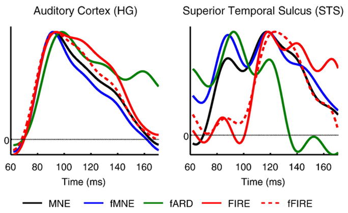
Estimated neural activity timecourses at the auditory cortex and STS using different methods.

Discussion

The coupling between the spatial and temporal domains in the joint E/MEG-fMRI analysis has restricted many previous models to operate on a coarse source space. The use of a regional neurovascular coupling model proposed in this paper reduces the computational burden, leading to a tractable reconstruction on a densely sampled source space, similar to that typically used in MNE.

In practice, it is often necessary to use slightly different experimental designs for fMRI and MEG. In this work, we used two types of experiments to test FIRE: (a) a somatosensory experiment with identical MEG and fMRI paradigms and (b) an auditory experiment, which provides an example of a situation where exact matching fMRI vs. MEG paradigms may be suboptimal. Specifically, in the auditory experiment we used a blocked sparse-sampling fMRI design to mitigate acoustical scanner noise; adding similar interleaved EPI noise/silent baseline periods would have made the corresponding MEG measurement simply too long for the subjects. These experimental designs were based on previous studies (Ahveninen et al., 2006; Jääskeläinen et al., 2004). Although the general activation patterns are the same across different modalities, we expect that minor discrepancies remain. Thus, the question on how well we can deal with such differences using FIRE depends on the underlying theoretical neurophysiological assumptions. One of the major advantages of FIRE is that its underlying generative model does not force perfect match in activations (Eq. (1)), avoiding excessive bias toward fMRI information.

As mentioned earlier, a more standard inference procedure for our graphical model would jointly consider J and Z as latent variables in the EM framework, while maximizing the log likelihood with respect to the model parameters Θ. Since [J, Z] and the measurement are jointly Gaussian given the model parameters Θ, the posterior probability distribution of the latent variables [J, Z] is also Gaussian, leading to a closed-form update. Similar to the derivations in Eq. (16), the M-step updates depend on the first- and second-order statistics of the latent variables, computed in the E-step. Since J is not fixed in this EM procedure, the estimate at each location depends on the estimate at all other locations in the source space, as opposed to the region-based estimation in Eq. (12) when J is fixed. Computing the second-order statistics involves solving NT_J + N systems of linear equations, each of which is of size NT_F + MT_J. In other words, we need to apply the conjugate gradient solver NT_J + N times, exacerbating the memory and runtime requirements for the procedure similar to the bottleneck step in our coordinate descent approach (Step ii-2 in the algorithm summary). Therefore, treating both J and Z as hidden variables is infeasible except for an extremely coarse discretization of the source space. Similarly, it is currently computationally infeasible to compute the variance of vec(Ĵ), since it requires applying the conjugate gradient solver NT_J times. Instead of the variance of the estimate, we provide an alternative way to study the sensitivity of the solver through Monte Carlo simulations.

The estimation of u_k and v_k is closely related to the Canonical Correlation Analysis (CCA), which seeks vectors for projecting two high dimensional data sets ({Ĵ_n}_{n Pk} and {f_n}_{n Pk} in our case) to a low dimensional space so as to maximize the correlation coefficient between the resulting projection coordinates. The probabilistic interpretation of CCA, established in Bach and Jordan (2005), offers a generative perspective on the method. Moreover, the probabilistic interpretation also helps to naturally extend the CCA model by incorporating prior information such as prior distributions on the waveforms U and V.

Since the cost function is not convex, our method depends on the initialization. MNE estimate is a reasonable choice for initialization since it is unbiased while fMNE is a good alternative as MNE estimates may be too diffuse in certain brain regions. Moreover, maximizing the cost function does not necessarily correspond to the best ROC performance. For the Monte Carlo simulation trials where value of the likelihood achieved by fFIRE is greater than that of FIRE, the ROC performance of fFIRE is often better than that of FIRE. A good ROC performance indicates the results are close to the ground truth, but it is not perfectly correlated with the likelihood values, which are based on an approximate model inference.

The results reported above are based on Freesurfer parcellation with 35 parcels per hemisphere. We also tried another parcellation provided by FreeSurfer with 85 parcels per hemisphere, and the resulting detection accuracy is similar to those obtained using the 35 parcel setting. For the estimated timecourses, the results using the 85 parcel setting is slightly less stable compared to the results computed using the 35 parcel setting, reflected by a slightly smaller correlation coefficient between the estimated timecourses and the ground truth timecourses. FIRE is also compatible with a data-driven parcellation. However, this approach may create an undesirable bias due to the use of the data in both parcel generation and current estimation. This bias can be avoided if the data-driven parcellation is obtained using a separate independent functional data set.

Our neurovascular coupling model is designed for fixed-orientation current estimates, since the latent-variable model assumes that the spatial concordance of neural and vascular activities is characterized by a scalar. For free-orientation current estimates, the neurovascular coupling model would have to be adjusted to handle the correspondence between the current flow in three directions and a single vascular activation timecourse at a certain location. Moreover, FIRE assumes a single activation waveform pair, u and v, in a region. The validity of this assumption depends on the size of the region and the distance between two activation sources. We cannot easily extend FIRE to multiple activation waveform pairs per region, since such an extension does not capture the fact that the shape of the vascular activation timecourses from two distinct sources is often highly similar but the neural processes are different. In the situation where there are two distinct current sources in one region, our preliminary results demonstrate that FIRE can localize the two current sources, but the estimated timecourses are combinations of the true timecourses. We defer the extension for free-orientation estimate and the extension for multiple activation sources per region to future work.

Conclusions

In contrast to most joint E/MEG-fMRI models, we explicitly take into account the inherent differences in the data measured by E/MEG and fMRI, allowing for common situations in real experiments where either neural or vascular activity is silent. The current source estimates can be computed efficiently with an iterative procedure which bears similarity to the re-weighted MNE methods, except that the weights are based on both the current estimates in the last iteration and the fMRI data via the proposed spatial neurovascular coupling model. This construction of the weights reduces the excessive sensitivity to fMRI present in many joint E/MEG-fMRI analysis methods and leads to more accurate current estimates as demonstrated by our experimental results with both simulated and human data.

Appendix A

In this Appendix, we describe the estimation procedure for J based on the standard jointly Gaussian distribution. As mentioned before, W and J are jointly Gaussian. For fixed Θ̂, if we define

$$\mathbf{W}={\left[{\mathbf{f}}^T(1),\dots ,{\mathbf{f}}^T(T_{\mathbf{F}}),{\mathbf{y}}^T(1),\dots ,{\mathbf{y}}^T(T_{\mathbf{J}})\right]}^T,$$ (20)

then

$$\mathbf{W}\sim \mathcal{N}(0,{\mathbf{\Gamma }}_{\mathbf{W}})=\mathcal{N}\left(0,\left[\begin{array}{cc}{\mathbf{\Gamma }}_{\mathbf{F}}& {\mathbf{\Gamma }}_{\mathbf{F},\mathbf{Y}}\\ {\mathbf{\Gamma }}_{\mathbf{F},\mathbf{Y}}^T& {\mathbf{\Gamma }}_{\mathbf{Y}}\end{array}\right]\right)$$ (21)

where Γ_X,Y are the covariance matrix of the corresponding random variables X and Y. Furthermore,

$${\left[{\mathbf{W}}^T,{\mathbf{j}}^T(1),\dots ,{\mathbf{j}}^T(T_{\mathbf{J}})\right]}^T\sim \mathcal{N}\left(0,\left[\begin{array}{cc}{\mathbf{\Gamma }}_{\mathbf{W}}& {\mathbf{\Gamma }}_{\mathbf{W},\mathbf{J}}\\ {\mathbf{\Gamma }}_{\mathbf{W},\mathbf{J}}^T& {\mathbf{\Gamma }}_{\mathbf{J}}\end{array}\right]\right).$$ (22)

Here, we only show the derivations of the covariance matrices for a single region (K = 1). The extension to multiple regions is straightforward. Based on the definition of covariance, we obtain

$$\begin{array}{l}{\mathbf{\Gamma }}_{\mathbf{F}}=\left(\mathbf{v}{\mathbf{v}}^T+{\xi }^2{\mathbf{I}}_{T_{\mathbf{F}}}\right)\otimes {\mathbf{I}}_N\\ {\mathbf{\Gamma }}_{\mathbf{Y}}=\left(\mathbf{u}{\mathbf{u}}^T+{\eta }^2{\mathbf{I}}_{T_{\mathbf{J}}}\right)\otimes \mathbf{A}{\mathbf{A}}^T+{\mathbf{I}}_{M{T}_{\mathbf{J}}}\\ {\mathbf{\Gamma }}_{\mathbf{F},\mathbf{Y}}=\left(\mathbf{v}{\mathbf{u}}^T\right)\otimes {\mathbf{A}}^T\\ {\mathbf{\Gamma }}_{\mathbf{W},\mathbf{J}}=\left[\left(\mathbf{v}{\mathbf{u}}^T\right)\otimes {\mathbf{I}}_N,\left(\mathbf{u}{\mathbf{u}}^T+{\eta }^2{\mathbf{I}}_{T_{\mathbf{J}}}\right)\otimes \mathbf{A}\right]\end{array}$$ (23)

where I_N indicates an identity matrix of size N. Eq. (25) assumes a normalized E/MEG sensory noise with unit variance. Matrix Kronecker product ⊗ stems from the interactions between space and time in the model.

We can then express the conditional distribution p(J|W) using the Bayes’ rule:

$$p(\text{vec}(\mathbf{J})\mid \mathbf{W})=\frac{p(\mathbf{W},\text{vec}(\mathbf{J}))}{p(\mathbf{W})}=\mathcal{N}\left({\mathbf{\Gamma }}_{\mathbf{W},\mathbf{J}}^T{\mathbf{\Gamma }}_{\mathbf{W}}^{-1}\mathbf{W},{\mathbf{\Gamma }}_{\mathbf{J}}-{\mathbf{\Gamma }}_{\mathbf{W},\mathbf{J}}^T{\mathbf{\Gamma }}_{\mathbf{W}}^{-1}{\mathbf{\Gamma }}_{\mathbf{W},\mathbf{J}}\right).$$

Appendix B

In this Appendix, we derive the M-step for estimating Θ. When Ĵ is fixed, we employ the EM algorithm to optimize the model parameters θ_k = [u_k, v_k, γ_k] for each region separately:

$${\widehat{\theta }}_k=arg\mathit{ma}{x}_{{\theta }_k}{\int }_{{\underset{\_}{\mathbf{z}}}_k}q\left({\underset{\_}{\mathbf{z}}}_k\right)logp\left({\left\{{\mathbf{f}}_n,{\widehat{\mathbf{j}}}_n\right\}}_{n\in P_k},z_n;{\theta }_k\right)d{\underset{\_}{\mathbf{z}}}_k$$ (24)

$$\begin{array}{l}=arg\underset{{\theta }_k}{max}{\int }_{{\underset{\_}{\mathbf{z}}}_k}q\left({\underset{\_}{\mathbf{z}}}_k\right)logp\left({\left\{{\mathbf{f}}_n,{\widehat{\mathbf{j}}}_n\right\}}_{n\in P_k}\mid z_n;{\mathbf{u}}_k,{\mathbf{v}}_k\right)p\left({\underset{\_}{\mathbf{z}}}_k;{\gamma }_k\right)d{\underset{\_}{\mathbf{z}}}_k\\ =arg\underset{{\theta }_k}{max}{\int }_{{\underset{\_}{\mathbf{z}}}_k}q\left({\underset{\_}{\mathbf{z}}}_k\right)\sum _{n\in P_k}\left(logp({\mathbf{f}}_n\mid z_n;{\mathbf{v}}_k)+logp({\widehat{\mathbf{j}}}_n\mid z_n;{\mathbf{u}}_k)\right)d{\underset{\_}{\mathbf{z}}}_k+{\int }_{{\underset{\_}{\mathbf{z}}}_k}q\left({\underset{\_}{\mathbf{z}}}_k\right)logp\left({\underset{\_}{\mathbf{z}}}_k;{\gamma }_k\right)d{\underset{\_}{\mathbf{z}}}_k\\ =arg{max}_{{\theta }_k}\left[-\frac{1}{2}\sum _{n\in P_k}{\langle {\left|\right|{\mathbf{f}}_n-z_n{\mathbf{v}}_k\left|\right|}^2\rangle }_q-\frac{1}{2}\sum _{n\in P_k}{\langle {\left|\right|{\widehat{\mathbf{j}}}_n-z_n{\mathbf{u}}_k\left|\right|}^2\rangle }_q-\frac{1}{2}\frac{\langle {\underset{\_}{\mathbf{z}}}_k^T{\mathbf{\Gamma }}_k^{-1}{\underset{\_}{\mathbf{z}}}_k\rangle }{{\gamma }_k^2}-N_{k}log{\gamma }_k^2\right]\end{array}$$ (25)

$$\begin{array}{l}=\underset{{\theta }_k}{argmax}\left[N_k{\mathbf{v}}_k^T{\mathbf{f}}_n{\langle z_n\rangle }_q-\frac{N_k}{2}{\mathbf{v}}_k^T{\mathbf{v}}_k{\langle z_n^2\rangle }_q+N_k{\mathbf{u}}_k^T{\widehat{\mathbf{j}}}_n{\langle z_n\rangle }_q-\frac{N_k}{2}{\mathbf{u}}_k^T{\mathbf{u}}_k{\langle z_n^2\rangle }_q-\frac{1}{2}\frac{{\langle {\underset{\_}{\mathbf{z}}}_k^T{\mathbf{\Gamma }}_k^{-1}{\underset{\_}{\mathbf{z}}}_k\rangle }_q}{{\gamma }_k^2}-N_{k}log{\gamma }_k^2\right]\\ =\underset{{\theta }_k}{argmax}\left[N_k\left({\mathbf{v}}_k^T{\mathbf{f}}_n+{\mathbf{u}}_k^T{\widehat{\mathbf{j}}}_n\right),{\langle z_n\rangle }_q-\frac{N_k}{2}\left({\mathbf{v}}_k^T{\mathbf{v}}_k+{\mathbf{u}}_k^T{\mathbf{u}}_k\right),{\langle z_n^2\rangle }_q,-\frac{1}{2}\frac{{\langle {\underset{\_}{\mathbf{z}}}_k^T{\mathbf{\Gamma }}_k^{-1}{\underset{\_}{\mathbf{z}}}_k\rangle }_q}{{\gamma }_k^2},-,N_{k}log{\gamma }_k^2\right].\end{array}$$ (26)

Eq. (25) is obtained with parameter setting ${\eta }_k^2={\xi }_k^2=1$ as discussed in Methods. Therefore, we only need to updates <z_n>_q, ${\langle z_n^2\rangle }_q$, and ${\langle {\underset{\_}{\mathbf{z}}}_k^{\text{T}}{\mathrm{\Gamma }}_k^{-1}{\underset{\_}{\mathbf{z}}}_k\rangle }_q$ in the E-step. By equating the derivatives of Eq. (26) with respect to u_k, v_k, and ${\gamma }_k^2$ to zero, we obtain the M-step updates in Eq. (16).

References

- Ahlfors S, Simpson G. Geometrical interpretation of fMRI-guided MEG/EEG inverse estimates. NeuroImage. 2004;22:323–332. doi: 10.1016/j.neuroimage.2003.12.044. [DOI] [PubMed] [Google Scholar]
- Ahveninen J, Jaaskelainen IP, Raij T, Bonmassar G, Devore S, Hamalainen M, Levanen S, Lin FH, Sams M, Shinn-Cunningham BG, Witzel T, Belliveau JW. Task-modulated “what” and “where” pathways in human auditory cortex. Proc Natl Acad Sci U S A. 2006;103:14608–14613. doi: 10.1073/pnas.0510480103. [DOI] [PMC free article] [PubMed] [Google Scholar]
- Altmann CF, Henning M, Doring MK, Kaiser J. Effects of feature-selective attention on auditory pattern and location processing. NeuroImage. 2008;41:69–79. doi: 10.1016/j.neuroimage.2008.02.013. [DOI] [PubMed] [Google Scholar]
- Bach F, Jordan M. Technical Report 688. UC Berkeley: 2005. A probabilistic interpretation of canonical correlation analysis. [Google Scholar]
- Baillet S, Mosher J, Leahy R. Electromagnetic brain mapping. IEEE Signal Proc Mag. 2001;18:14–30. [Google Scholar]
- Daunizeau J, Grova C, Marrelec G, Mattout J, Jbabdi S, Pelegrini-Issac M, Lina J, Benali H. Symmetrical event-related EEG/fMRI information fusion in a variational Bayesian framework. NeuroImage. 2007;36:69–87. doi: 10.1016/j.neuroimage.2007.01.044. [DOI] [PubMed] [Google Scholar]
- Dempster A, Laird N, Rubin D. Maximum likelihood from incomplete data via the EM algorithm. J R Stat Soc B. 1977;39:1–38. [Google Scholar]
- Deneux T, Faugeras O. EEG-fMRI Fusion of Non-triggered Data using Kalman Filtering. 2006. [Google Scholar]
- Fischl B, Salat D, Busa E, Albert M, Dieterich M, Haselgrove C, van der Kouwe A, Killiany R, Kennedy D, Klaveness S, Montillo A, Makris N, Rosen B, Dale A. Whole brain segmentation: automated labeling of neuroanatomical structures in the human brain. Neuron. 2002;33:341–355. doi: 10.1016/s0896-6273(02)00569-x. [DOI] [PubMed] [Google Scholar]
- Fujimaki N, Hayakawa T, Nielsen M, Knösche TR, Miyauchi S. An fMRI-constrained MEG source analysis with procedures for dividing and grouping activation. NeuroImage. 2002;17:324–343. doi: 10.1006/nimg.2002.1160. [DOI] [PubMed] [Google Scholar]
- George JS, Aine CJ, Mosher JC, Schmidt DM, Ranken DM, Schlitt HA, Wood CC, Lewine JD, Sanders JA, Belliveau JW. Mapping function in the human brain with magnetoencephalography, anatomical magnetic resonance imaging, and functional magnetic resonance imaging. J Clin Neurophysiol. 1995;12:406–431. doi: 10.1097/00004691-199509010-00002. [DOI] [PubMed] [Google Scholar]
- Gorodnitsky I, Rao B. Sparse signal reconstruction from limited data using FOCUSS: a re-weighted MNE algorithm. IEEE Trans Signal Process. 1997;45:600–616. [Google Scholar]
- Hadamard J. Princeton University Bulletin. 1902. Sur les Problems aux Derivees Partielles et Leur Signification Physique; pp. 49–52. [Google Scholar]
- Hall DA, Haggard MP, Akeroyd MA, Palmer AR, Summerfield AQ, Elliott MR, Gurney EM, Bowtell RW. “Sparse” temporal sampling in auditory fMRI. Hum Brain Mapp. 1999;7:213–223. doi: 10.1002/(SICI)1097-0193(1999)7:3<213::AID-HBM5>3.0.CO;2-N. [DOI] [PMC free article] [PubMed] [Google Scholar]
- Hämäläinen MS, Ilmoniemi R. Interpreting measured magnetic fields of the brain: estimates of current distributions. Technical Report TKK-F-A559 1984 [Google Scholar]
- Hämäläinen M, Sarvas J. Realistic conductivity geometry model of the human head for interpretation of neuromagnetic data. IEEE Biomed Eng. 1989;36:165–171. doi: 10.1109/10.16463. [DOI] [PubMed] [Google Scholar]
- Hämäläinen MS, Hari R, Ilmoniemi R, Knuutila J, Lounasmaa OV. Magnetoencephalography — theory, instrumentation, and applications to noninvasive studies of the working human brain. Rev Mod Phys. 1993;65:413–497. [Google Scholar]
- Hari R, Forss N. Magnetoencephalography in the study of human somatosensory cortical processing. Philos Trans R Soc Lond B. 1999;354:1145–1154. doi: 10.1098/rstb.1999.0470. [DOI] [PMC free article] [PubMed] [Google Scholar]
- Hart HC, Palmer AR, Hall DA. Heschl’s gyrus is more sensitive to tone level than non-primary auditory cortex. Hear Res. 2002;171:177–190. doi: 10.1016/s0378-5955(02)00498-7. [DOI] [PubMed] [Google Scholar]
- Jääskeläinen IP, Ahveninen J, Bonmassar G, Dale AM, Ilmoniemi RJ, Levänen S, Lin FH, May P, Melcher J, Stuffiebeam S, Tiitinen H, Belliveau JW. Human posterior auditory cortex gates novel sounds to consciousness. PNAS. 2004;101:6809–6814. doi: 10.1073/pnas.0303760101. [DOI] [PMC free article] [PubMed] [Google Scholar]
- Jun SC, George JS, Kim W, Paré-Blagoev J, Plis S, Ranken DM, Schmidt DM. Bayesian brain source imaging based on combined MEG/EEG and fMRI using MCMC. NeuroImage. 2008;40:1581–1594. doi: 10.1016/j.neuroimage.2007.12.029. [DOI] [PMC free article] [PubMed] [Google Scholar]
- Liu A, Belliveau J, Dale A. Spatiotemporal imaging of human brain activity using functional MRI constrained magnetoencephalography data: Monte Carlo simulations. PNAS. 1998;95:8945–8950. doi: 10.1073/pnas.95.15.8945. [DOI] [PMC free article] [PubMed] [Google Scholar]
- Liu Z, He B. fMRI-EEG integrated cortical source imaging by use of time-variant spatial constraints. NeuroImage. 2008;39:1198–1214. doi: 10.1016/j.neuroimage.2007.10.003. [DOI] [PMC free article] [PubMed] [Google Scholar]
- Logothetis N, Wandell B. Interpreting the BOLD signal. Annu Rev Physiol. 2004;66:735–769. doi: 10.1146/annurev.physiol.66.082602.092845. [DOI] [PubMed] [Google Scholar]
- Lu ZL, Williamson SJ, Kaufman L. Human auditory primary and association cortex have differing lifetimes for activation traces. Brain Res. 1992;572:236–241. doi: 10.1016/0006-8993(92)90475-o. [DOI] [PubMed] [Google Scholar]
- Mosher JC, Lewis PS, Leahy RM. Multiple dipole modeling and localization from spatiotemporal MEG data. IEEE Trans Biomed Eng. 1992;39:541–557. doi: 10.1109/10.141192. [DOI] [PubMed] [Google Scholar]
- Oostendorp TF, Van Oosterom A. Source parameter estimation in inhomogeneous volume conductors of arbitrary shape. IEEE Trans Biomed Eng. 1989;36:382–391. doi: 10.1109/10.19859. [DOI] [PubMed] [Google Scholar]
- Ou W, Hämäläinen M, Golland P. A distributed spatiotemporal EEG/MEG inverse solver. NeuroImage. 2009a;44:932–946. doi: 10.1016/j.neuroimage.2008.05.063. [DOI] [PMC free article] [PubMed] [Google Scholar]
- Ou W, Nissilä I, Radhakrishnan H, Boas D, Hämäläinen M, Franceschini M. Study of neurovascular coupling in humans via simultaneous magnetoencephalography and diffuse optical imaging acquisition. NeuroImage. 2009b;46:624–632. doi: 10.1016/j.neuroimage.2009.03.008. [DOI] [PMC free article] [PubMed] [Google Scholar]
- Ou W, Nummenmaa A, Hämäläinen M, Golland P. Multimodal functional imaging using fMRI-informed regional EEG/MEG source estimation. Proc. IPMI: International Conference on Information Processing and Medical Imaging; LNCS; 2009c. pp. 88–100. [Google Scholar]
- Pascual-Marqui R, Michel C, Lehmann D. Low resolution electromagnetic tomography: a new method for localizing electrical activity in the brain. Int J Psychophysiol. 1994;18:49–65. doi: 10.1016/0167-8760(84)90014-x. [DOI] [PubMed] [Google Scholar]
- Rauschecker JP. Cortical processing of complex sounds. Curr Opin Neurobiol. 1998;8:516–521. doi: 10.1016/s0959-4388(98)80040-8. [DOI] [PubMed] [Google Scholar]
- Sato M, Yoshioka T, Kajihara S, Toyama K, Goda N, Doya K, Kawato M. Hierarchical Bayesian estimation for MEG inverse problem. NeuroImage. 2004;23:806–826. doi: 10.1016/j.neuroimage.2004.06.037. [DOI] [PubMed] [Google Scholar]
- Scherg M, Von Cramon D. Two bilateral sources of the late AEP as identified by a spatiotemporal dipole model. Electroencephalogr Clin Neurophysiol. 1985;62:32–44. doi: 10.1016/0168-5597(85)90033-4. [DOI] [PubMed] [Google Scholar]
- Tipping M, Bishop C. Probabilistic principal component analysis. J R Stat Soc B. 1999;61:611–622. [Google Scholar]
- Uutela K, Hämäläinen MS, Somersalo E. Visualization of magnetoencephalographic data using minimum current estimates. NeuroImage. 1999;10:173–180. doi: 10.1006/nimg.1999.0454. [DOI] [PubMed] [Google Scholar]
- Vanni S, Warnking J, Dojat M, Delon-Martin C, Bullier J, Segebarth C. Sequence of pattern onset responses in the human visual areas: an fMRI constrained VEP source analysis. NeuroImage. 2004;21:801–817. doi: 10.1016/j.neuroimage.2003.10.047. [DOI] [PubMed] [Google Scholar]
- Wang JZ, Williamson SJ, Kaufman L. Magnetic source imaging based on the minimum-norm least-squares inverse. Brain Topogr. 1993;5:365–371. doi: 10.1007/BF01128692. [DOI] [PubMed] [Google Scholar]
- Williamson SJ, Lu ZL, Karron D, Kaufman L. Advantages and limitations of magnetic source imaging. Brain Topogr. 1991;4:169–180. doi: 10.1007/BF01132773. [DOI] [PubMed] [Google Scholar]
- Wipf D, Rao B. Sparse Bayesian learning for basis selection. IEEE Trans Signal Process. 2004;52:2153–2164. [Google Scholar]
- Wipf D, Nagarajan S. A unified Bayesian framework for MEG/EEG source imaging. NeuroImage. 2009;44:947–966. doi: 10.1016/j.neuroimage.2008.02.059. [DOI] [PMC free article] [PubMed] [Google Scholar]
- Wood CC. Application of dipole localization methods to source identification of human evoked potentials. Ann NY Acad Sci. 1982;388:139–155. doi: 10.1111/j.1749-6632.1982.tb50789.x. [DOI] [PubMed] [Google Scholar]